Implementing GANs from Scratch in PyTorch
1. Generator and Discriminator Networks
Generator and Discriminator Networks
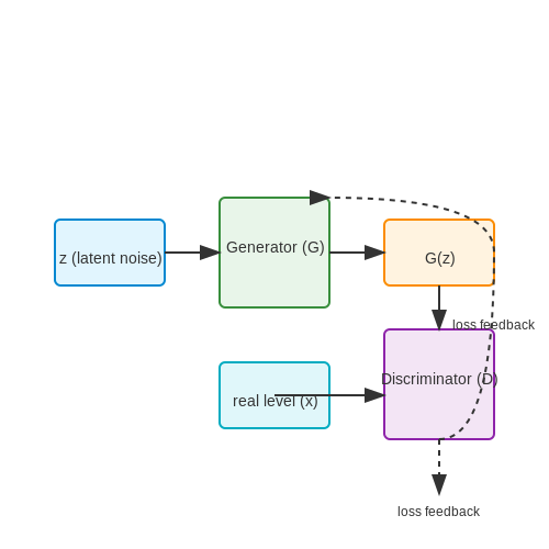
The generator and discriminator are the two core neural networks in a GAN. The generator G maps a latent noise vector z to synthetic data samples, while the discriminator D evaluates whether an input sample is real or generated. Their adversarial interplay drives the learning process.
Generator Architecture
The generator is typically a deep neural network that transforms a low-dimensional latent vector z ∈ ℝd into a high-dimensional output resembling the training data. For image generation, transposed convolutional layers are commonly used to progressively upsample the input:
where Wi are learnable weights, bi are biases, φ is a nonlinear activation (commonly LeakyReLU), and σ is the output activation (e.g., tanh for images normalized to [-1, 1]). Batch normalization helps stabilize training by normalizing layer inputs.
Discriminator Architecture
The discriminator is a binary classifier that takes either real or generated samples as input and outputs a probability D(x) ∈ [0,1] indicating authenticity. For images, it typically uses strided convolutions to downsample the input:
where Vi and ci are learnable parameters, and ψ is typically LeakyReLU. Spectral normalization can be applied to the weights to enforce Lipschitz continuity, improving training stability.
Implementation in PyTorch
Below is a PyTorch implementation of a DCGAN-style generator and discriminator for 64×64 RGB images:
import torch
import torch.nn as nn

class Generator(nn.Module):
    def __init__(self, latent_dim=100):
        super().__init__()
        self.main = nn.Sequential(
            nn.ConvTranspose2d(latent_dim, 512, 4, 1, 0, bias=False),
            nn.BatchNorm2d(512),
            nn.ReLU(True),
            nn.ConvTranspose2d(512, 256, 4, 2, 1, bias=False),
            nn.BatchNorm2d(256),
            nn.ReLU(True),
            nn.ConvTranspose2d(256, 128, 4, 2, 1, bias=False),
            nn.BatchNorm2d(128),
            nn.ReLU(True),
            nn.ConvTranspose2d(128, 64, 4, 2, 1, bias=False),
            nn.BatchNorm2d(64),
            nn.ReLU(True),
            nn.ConvTranspose2d(64, 3, 4, 2, 1, bias=False),
            nn.Tanh()
        )

    def forward(self, z):
        return self.main(z.unsqueeze(-1).unsqueeze(-1))

class Discriminator(nn.Module):
    def __init__(self):
        super().__init__()
        self.main = nn.Sequential(
            nn.Conv2d(3, 64, 4, 2, 1, bias=False),
            nn.LeakyReLU(0.2, inplace=True),
            nn.Conv2d(64, 128, 4, 2, 1, bias=False),
            nn.BatchNorm2d(128),
            nn.LeakyReLU(0.2, inplace=True),
            nn.Conv2d(128, 256, 4, 2, 1, bias=False),
            nn.BatchNorm2d(256),
            nn.LeakyReLU(0.2, inplace=True),
            nn.Conv2d(256, 512, 4, 2, 1, bias=False),
            nn.BatchNorm2d(512),
            nn.LeakyReLU(0.2, inplace=True),
            nn.Conv2d(512, 1, 4, 1, 0, bias=False),
            nn.Sigmoid()
        )

    def forward(self, x):
        return self.main(x).view(-1)
Critical Design Considerations
- Normalization: BatchNorm in the generator helps gradient flow but can cause instability in the discriminator. InstanceNorm or LayerNorm are alternatives.
- Activation Functions: LeakyReLU (α=0.2) prevents dead neurons in discriminators. Output activations must match data normalization (e.g., tanh for [-1,1]).
- Capacity Balance: The discriminator should not become too strong too quickly, as this can vanish gradients for the generator.

Adversarial Training Dynamics
The core challenge in training GANs stems from the adversarial min-max game between the generator G and discriminator D, formalized as:
This formulation creates a dynamic equilibrium where D tries to distinguish real from fake samples while G attempts to fool D. The training process alternates between updating D to maximize the probability of assigning correct labels and updating G to minimize $$\log(1 - D(G(z)))$$.
Gradient Analysis
The discriminator's gradient with respect to its parameters $$\theta_d$$ is:
while the generator's gradient is:
Early in training, when G is poor, $$\log(1 - D(G(z)))$$ saturates, providing weak gradients. This motivates using $$- \log D(G(z))$$ as an alternative objective for G.
Nash Equilibrium Analysis
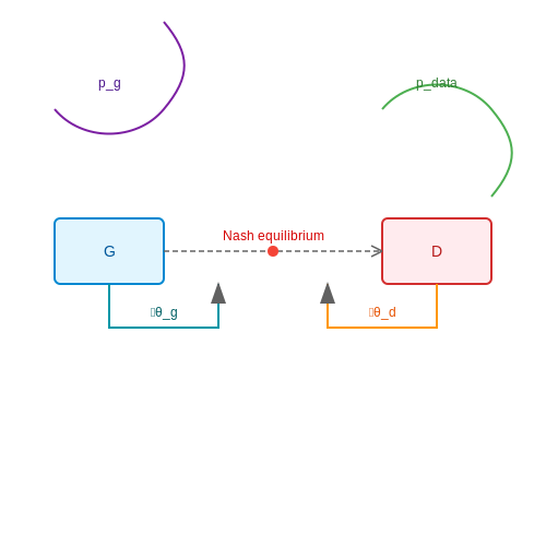
The optimal solution occurs at a Nash equilibrium where:
and $$p_g = p_{data}$$. However, achieving this equilibrium is challenging due to:
- Mode collapse: G produces limited varieties of samples
- Oscillations: Parameters may orbit the equilibrium without converging
- Vanishing gradients: When D becomes too confident
Training Stability Techniques
Modern GAN implementations employ several stabilization methods:
- Feature matching: Match statistics of intermediate layers
- Minibatch discrimination: Allow D to see multiple samples simultaneously
- Historical averaging: Incorporate past parameter values
- One-sided label smoothing: Replace 1s with 0.9 for real samples
The Wasserstein GAN (WGAN) formulation improves stability by using the Earth-Mover distance:
where $$\Pi(p_{data}, p_g)$$ denotes all joint distributions with marginals $$p_{data}$$ and $$p_g$$.
Practical Implementation Considerations
In PyTorch, the adversarial training loop requires careful balancing:
for epoch in range(num_epochs):
    for real_data, _ in dataloader:
        # Update D
        optimizer_D.zero_grad()
        z = torch.randn(batch_size, latent_dim)
        fake_data = generator(z)
        real_loss = adversarial_loss(discriminator(real_data), real_labels)
        fake_loss = adversarial_loss(discriminator(fake_data.detach()), fake_labels)
        d_loss = (real_loss + fake_loss) / 2
        d_loss.backward()
        optimizer_D.step()

        # Update G
        optimizer_G.zero_grad()
        gen_loss = adversarial_loss(discriminator(fake_data), real_labels)
        gen_loss.backward()
        optimizer_G.step()
The discriminator's learning rate is typically set lower than the generator's (e.g., 0.0001 vs 0.0004) to prevent it from becoming too strong too quickly. Batch normalization helps prevent mode collapse by ensuring no single sample dominates the gradient updates.
1.3 Common Challenges in GAN Training
Mode Collapse
Mode collapse occurs when the generator produces a limited variety of outputs, often converging to a few modes of the data distribution. The discriminator fails to penalize this behavior, leading to repetitive or nearly identical samples. Mathematically, this can be understood as the generator optimizing for a subset of the data distribution where the discriminator is weakest:
When mode collapse happens, the generator exploits specific weaknesses in the discriminator's decision boundaries, causing the loss landscape to become degenerate. Techniques like minibatch discrimination or unrolled GANs can mitigate this by forcing the discriminator to evaluate samples in batches rather than individually.
Vanishing Gradients
GAN training often suffers from vanishing gradients, particularly when the discriminator becomes too strong. If the discriminator achieves near-perfect accuracy, the generator receives minimal gradient signals, stalling its learning. This is evident in the gradient of the generator's loss:
When \(D(G(z))\) approaches 0, the gradient vanishes, making updates ineffective. Using alternative loss functions like the non-saturating loss, where the generator maximizes \(\log D(G(z))\), can alleviate this issue by providing stronger gradients early in training.
Oscillations and Instability
GAN dynamics often exhibit oscillatory behavior, where the generator and discriminator fail to converge to a stable equilibrium. This arises because the optimization process is a two-player minimax game rather than a cooperative objective. The discriminator and generator may continuously adapt to each other's strategies without reaching a Nash equilibrium. Techniques like gradient penalty (as used in WGAN-GP) or spectral normalization can stabilize training by enforcing Lipschitz constraints on the discriminator.
Hyperparameter Sensitivity
GANs are notoriously sensitive to hyperparameters, including learning rates, batch sizes, and architecture choices. Small changes can lead to drastically different outcomes, such as divergence or mode collapse. For instance, the balance between the generator and discriminator learning rates is critical. If the discriminator learns too quickly, it can overpower the generator, while a slow discriminator may fail to provide meaningful feedback. Adaptive optimizers like Adam with tuned \(eta_1\) and \(eta_2\) can help, but empirical tuning is often necessary.
Evaluation Difficulties
Quantifying GAN performance remains challenging due to the lack of a definitive metric. Common evaluation methods include:
- Inception Score (IS): Measures the diversity and quality of generated images using a pretrained Inception-v3 model.
- Fréchet Inception Distance (FID): Compares the statistics of generated and real data in feature space.
- Precision and Recall: Evaluates the coverage and fidelity of generated samples relative to the true data distribution.
However, these metrics have limitations. For example, IS can be fooled by generators producing unrealistic but high-confidence samples, while FID assumes Gaussian feature distributions, which may not hold in practice.
2. Installing PyTorch and Dependencies
2.1 Installing PyTorch and Dependencies
PyTorch is the foundational framework for implementing GANs, offering dynamic computation graphs and GPU acceleration. Begin by verifying CUDA compatibility if leveraging GPU support. Run nvidia-smi in the terminal to confirm CUDA version and GPU driver status. PyTorch installation varies based on the system configuration:
CUDA-Enabled Installation
For GPU acceleration, install PyTorch with CUDA support matching your driver version. Use the official PyTorch command generator to ensure compatibility:
conda install pytorch torchvision torchaudio cudatoolkit=11.6 -c pytorch -c conda-forgeCPU-Only Installation
If GPU support is unavailable, install the CPU-only variant:
conda install pytorch torchvision torchaudio cpuonly -c pytorchCritical Dependencies
GAN implementations often require additional libraries for data handling and visualization:
- NumPy: For numerical operations on tensors outside PyTorch.
- Matplotlib: To visualize generated images and loss curves.
- torchvision: Provides datasets, transforms, and pretrained models.
pip install numpy matplotlib torchvisionVersion Verification
Confirm successful installation by checking PyTorch version and CUDA availability in a Python shell:
import torch
print(torch.__version__)  # Expected output: e.g., '1.12.1'
print(torch.cuda.is_available())  # Should return True for GPU support
Handling Common Issues
Mismatched CUDA versions are a frequent source of installation failures. If torch.cuda.is_available() returns False, reinstall PyTorch with a CUDA version matching the system's driver. For Conda environments, ensure no conflicting packages exist by creating a fresh environment:
conda create -n gan_env python=3.9
conda activate gan_env
2.2 Configuring GPU Support (Optional)
PyTorch provides native CUDA support for accelerating tensor operations on NVIDIA GPUs. To leverage this for GAN training, we first verify GPU availability and then modify the model and data pipeline accordingly.
Checking GPU Availability
Before proceeding, confirm CUDA-capable devices are accessible via torch.cuda:
import torch
print(f"CUDA available: {torch.cuda.is_available()}")
print(f"Device count: {torch.cuda.device_count()}")
print(f"Current device: {torch.cuda.current_device()}")
print(f"Device name: {torch.cuda.get_device_name(0)}")
Device-Agnostic Code Implementation
For portable code that works on both CPU and GPU, create a device handle:
device = torch.device("cuda:0" if torch.cuda.is_available() else "cpu")Model Parallelization
Transfer generator and discriminator models to the selected device. This includes all learnable parameters:
generator = Generator().to(device)
discriminator = Discriminator().to(device)
Data Pipeline Optimization
Enable pinned memory for faster host-to-device transfers when using DataLoader:
train_loader = DataLoader(
    dataset,
    batch_size=64,
    shuffle=True,
    pin_memory=True,  # Enables faster CUDA transfer
    num_workers=4
)
Mixed Precision Training
For Volta/Turing/Ampere GPUs, enable automatic mixed precision (AMP) to reduce memory usage and increase throughput:
scaler = torch.cuda.amp.GradScaler()

with torch.cuda.amp.autocast():
    # Forward pass
    real_output = discriminator(real_images)
    fake_output = discriminator(fake_images)

    # Loss calculation
    loss = criterion(real_output, fake_output)

# Backward pass with scaling
scaler.scale(loss).backward()
scaler.step(optimizer)
scaler.update()
Multi-GPU Training
For data parallelism across multiple GPUs, wrap models with DataParallel or DistributedDataParallel:
if torch.cuda.device_count() > 1:
    generator = nn.DataParallel(generator)
    discriminator = nn.DataParallel(discriminator)
Note that batch sizes should be adjusted proportionally to the number of GPUs when using parallelism.
2.3 Verifying the Setup with a Simple Example
Before training a full GAN, we validate our PyTorch implementation by testing the generator and discriminator on a simple synthetic dataset. This sanity check ensures proper gradient flow and basic functionality.
Creating a Synthetic 1D Gaussian Dataset
We generate 10,000 samples from a 1D Gaussian distribution with μ=5 and σ=1.5:
import torch
import numpy as np

# Generate real data (1D Gaussian)
real_data = torch.normal(mean=5.0, std=1.5, size=(10000,1))
Simplified Generator and Discriminator
We implement minimal versions of both networks:
# Generator maps noise→1D output
generator = torch.nn.Sequential(
    torch.nn.Linear(100, 50),
    torch.nn.ReLU(),
    torch.nn.Linear(50, 1)

# Discriminator maps 1D input→scalar probability
discriminator = torch.nn.Sequential(
    torch.nn.Linear(1, 50),
    torch.nn.LeakyReLU(0.2),
    torch.nn.Linear(50, 1),
    torch.nn.Sigmoid())
Validation Test Procedure
The verification test follows these steps:
- Feed Gaussian noise z ∼ N(0,1) through generator
- Pass both real and generated samples through discriminator
- Check output shapes and value ranges
- Verify gradients exist for both networks
# Forward pass test
z = torch.randn(64, 100)  # Batch of noise
fake_data = generator(z)
d_real = discriminator(real_data[:64])
d_fake = discriminator(fake_data)

# Backward pass test
loss = torch.nn.BCELoss()(d_real, torch.ones_like(d_real))
loss.backward()

print(f"Generator grad exists: {generator[0].weight.grad is not None}")
print(f"Discriminator grad exists: {discriminator[0].weight.grad is not None}")
Expected Output Verification
The test should confirm:
Successful verification shows the basic computational graph is properly connected and automatic differentiation is working. The discriminator should initially perform near chance (accuracy ≈0.5) since the generator hasn't been trained.
3. Designing the Architecture
3.1 Designing the Architecture
The architecture of a Generative Adversarial Network (GAN) consists of two primary components: the Generator (G) and the Discriminator (D). The generator synthesizes fake samples from random noise, while the discriminator evaluates whether a given sample is real (from the training dataset) or fake (produced by G). The adversarial training process optimizes both networks simultaneously, with G improving its ability to deceive D, and D refining its discrimination capabilities.
Generator Architecture
The generator typically employs a series of transposed convolutional layers (also called fractionally strided convolutions) to upsample low-dimensional noise into high-dimensional synthetic data. For a 64×64 RGB image generation task, the architecture may follow this structure:
- Input Layer: A fully connected layer that maps a latent noise vector z (e.g., 100 dimensions) to a higher-dimensional space.
- Hidden Layers: Multiple transposed convolutional layers with batch normalization and ReLU activation, progressively increasing spatial resolution while reducing channel depth.
- Output Layer: A transposed convolution with a tanh activation function, ensuring pixel values are scaled to [-1, 1] to match normalized input data.
Discriminator Architecture
The discriminator is a convolutional neural network (CNN) that classifies inputs as real or fake. Its design often mirrors the generator but in reverse:
- Input Layer: Accepts either real data (e.g., 64×64×3 tensor) or generator output.
- Hidden Layers: Convolutional layers with LeakyReLU activation (slope ≈ 0.2) and batch normalization, reducing spatial dimensions while increasing channel depth.
- Output Layer: A fully connected layer with sigmoid activation, producing a scalar probability (0 for fake, 1 for real).
Critical Design Considerations
GAN stability hinges on architectural choices:
- Normalization: Batch normalization in both networks mitigates internal covariate shift, accelerating convergence.
- Activation Functions: LeakyReLU in D prevents dead neurons, while tanh in G ensures bounded outputs.
- Dimensionality: The latent space dimension (z) balances expressiveness and computational cost—typically between 50 and 200.
PyTorch Implementation Skeleton
import torch
import torch.nn as nn

class Generator(nn.Module):
    def __init__(self, latent_dim=100, img_channels=3):
        super().__init__()
        self.main = nn.Sequential(
            nn.Linear(latent_dim, 256 * 8 * 8),
            nn.Unflatten(1, (256, 8, 8)),
            nn.ConvTranspose2d(256, 128, 4, 2, 1, bias=False),
            nn.BatchNorm2d(128),
            nn.ReLU(True),
            nn.ConvTranspose2d(128, 64, 4, 2, 1, bias=False),
            nn.BatchNorm2d(64),
            nn.ReLU(True),
            nn.ConvTranspose2d(64, img_channels, 4, 2, 1, bias=False),
            nn.Tanh()
        )

    def forward(self, z):
        return self.main(z)

class Discriminator(nn.Module):
    def __init__(self, img_channels=3):
        super().__init__()
        self.main = nn.Sequential(
            nn.Conv2d(img_channels, 64, 4, 2, 1, bias=False),
            nn.LeakyReLU(0.2, inplace=True),
            nn.Conv2d(64, 128, 4, 2, 1, bias=False),
            nn.BatchNorm2d(128),
            nn.LeakyReLU(0.2, inplace=True),
            nn.Conv2d(128, 256, 4, 2, 1, bias=False),
            nn.BatchNorm2d(256),
            nn.LeakyReLU(0.2, inplace=True),
            nn.Flatten(),
            nn.Linear(256 * 8 * 8, 1),
            nn.Sigmoid()
        )

    def forward(self, x):
        return self.main(x)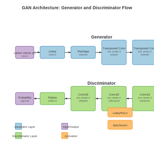
Implementing the Forward Pass
The forward pass in a GAN involves propagating input through both generator and discriminator networks while maintaining proper gradient flow. For the generator G, we transform random noise z into synthetic samples, while the discriminator D evaluates both real and generated samples.
Generator Forward Propagation
The generator's forward pass begins with sampling from the latent space:
where dz is the dimension of the latent vector. This noise vector passes through successive transposed convolutional layers with batch normalization and ReLU activations:
def forward(self, z):
    x = self.fc(z)
    x = x.view(-1, 512, 4, 4)  # Reshape for conv layers
    x = F.relu(self.bn1(self.conv1(x)))
    x = F.relu(self.bn2(self.conv2(x)))
    x = F.relu(self.bn3(self.conv3(x)))
    x = torch.tanh(self.conv4(x))  # Output in [-1,1]
    return x
Discriminator Forward Propagation
The discriminator processes both real (x) and fake (G(z)) samples through convolutional layers with leaky ReLU activations (α=0.2):
Implemented in PyTorch as:
def forward(self, x):
    x = self.conv1(x)
    x = F.leaky_relu(x, 0.2)
    x = self.conv2(x)
    x = F.leaky_relu(x, 0.2)
    x = x.view(-1, 128*7*7)  # Flatten
    x = self.fc(x)
    return torch.sigmoid(x)
Gradient Flow Considerations
During the forward pass, these architectural choices impact gradient behavior:
- Batch normalization in the generator helps maintain stable gradient magnitudes
- Leaky ReLU in the discriminator prevents dying gradients
- Tanh in the generator's output layer bounds values to [-1,1] matching normalized input data
The complete forward pass for one training iteration involves:
# Generate fake images
z = torch.randn(batch_size, latent_dim).to(device)
fake_images = generator(z)

# Discriminator forward pass
real_output = discriminator(real_images)
fake_output = discriminator(fake_images.detach())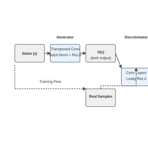
3.3 Initializing Weights for Stability
Weight initialization critically impacts GAN convergence by controlling gradient flow and preventing vanishing or exploding gradients. Poor initialization leads to mode collapse or oscillatory training dynamics. The key challenge lies in maintaining balanced gradients across both generator and discriminator networks throughout training.
Theoretical Foundations
Modern initialization schemes derive from analyzing signal propagation through deep networks. Consider a linear layer y = Wx + b with n inputs. The output variance should equal input variance to maintain stable gradients:
For ReLU activations (which zero out half the inputs), He initialization scales weights by √(2/n) to compensate:
For GANs, this becomes more nuanced as generator and discriminator require different scaling. The discriminator's gradient penalty term further modifies the optimal initialization.
PyTorch Implementation
Apply layer-specific initialization using torch.nn.init with these proven configurations:
def weights_init(m):
    classname = m.__class__.__name__
    if classname.find('Conv') != -1:
        nn.init.normal_(m.weight.data, 0.0, 0.02)
    elif classname.find('BatchNorm') != -1:
        nn.init.normal_(m.weight.data, 1.0, 0.02)
        nn.init.constant_(m.bias.data, 0)

# Apply to generator and discriminator
netG.apply(weights_init)
netD.apply(weights_init)
Advanced Techniques
For deep GAN architectures, consider these refinements:
- Orthogonal initialization: Ensures weight matrices preserve vector norms, particularly effective for recurrent connections in temporal GANs
- Layer-sequential unit-variance (LSUV): Iteratively scales weights until each layer's output achieves unit variance
- Spectral normalization: Constrains Lipschitz constants by normalizing weight matrices by their spectral norm
Empirical studies show that combining He initialization with spectral normalization yields the most stable training for ResNet-based GAN architectures, reducing the need for careful learning rate tuning.
4. Designing the Architecture
4.1 Designing the Architecture
Generator Network Structure
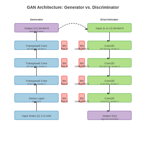
The generator G maps a latent noise vector z (typically sampled from a standard normal distribution z ∼ N(0, I)) to synthetic data samples x̃ = G(z). For image generation, G is implemented as a transposed convolutional network (also called a "deconvolutional network"). The architecture progressively upsamples the input noise through layers:
- Input Layer: A fully connected layer maps z ∈ ℝᵈ to a higher-dimensional tensor (e.g., 4×4×512 for DCGAN).
- Transposed Convolutional Blocks: Each block consists of:
- A transposed convolution (
nn.ConvTranspose2d) with stride ≥2 for upsampling. - Batch normalization (
nn.BatchNorm2d). - ReLU activation for intermediate layers; tanh for the final layer to bound outputs to [-1, 1].
- A transposed convolution (
Discriminator Network Structure
The discriminator D is a convolutional classifier that outputs a scalar probability D(x) ∈ [0, 1]. Its architecture mirrors G but in reverse:
- Convolutional Blocks: Each block includes:
- A convolution (
nn.Conv2d) with stride ≥2 for downsampling. - LeakyReLU activation (slope=0.2) to avoid vanishing gradients.
- Batch normalization except in the input layer.
- A convolution (
- Output Layer: A fully connected layer followed by a sigmoid (
nn.Sigmoid) for binary classification.
Critical Design Considerations
Architectural Symmetry: The discriminator’s downsampling strides must match the generator’s upsampling strides to ensure spatial compatibility. For a 64×64 output image, a common stack is:
# Generator (DCGAN-style)
self.main = nn.Sequential(
    nn.ConvTranspose2d(100, 512, 4, 1, 0, bias=False),
    nn.BatchNorm2d(512),
    nn.ReLU(),
    nn.ConvTranspose2d(512, 256, 4, 2, 1, bias=False),
    nn.BatchNorm2d(256),
    nn.ReLU(),
    nn.ConvTranspose2d(256, 128, 4, 2, 1, bias=False),
    nn.BatchNorm2d(128),
    nn.ReLU(),
    nn.ConvTranspose2d(128, 3, 4, 2, 1, bias=False),
    nn.Tanh()
)
Normalization: Batch normalization in both networks stabilizes training by preventing mode collapse. However, the discriminator’s input layer and generator’s output layer should omit it.
Loss Function: The vanilla GAN minimax objective is:
In practice, the generator is trained to maximize log(D(G(z))) instead of minimizing log(1 - D(G(z))) to avoid vanishing gradients early in training.
4.2 Implementing the Forward Pass
The forward pass in a GAN involves propagating input through both generator and discriminator networks while maintaining proper gradient flow. For the generator G, we transform random noise z into synthetic data samples, while the discriminator D processes both real and generated samples to produce classification probabilities.
Generator Forward Propagation
The generator's forward pass maps latent vectors z ∈ ℝd to data space through a series of transposed convolutions (or dense layers for simpler architectures):
Where gi are activation functions (typically ReLU for hidden layers, tanh for output in image generation), and Wi, bi are learnable parameters. In PyTorch, this translates to:
def forward(self, z):
    x = self.fc1(z)
    x = F.leaky_relu(x, 0.2)
    x = self.fc2(x)
    x = x.view(-1, 256, 4, 4)  # Reshape for conv layers
    x = F.relu(self.conv1(x))
    x = F.relu(self.conv2(x))
    x = torch.tanh(self.conv3(x))  # Normalize to [-1, 1]
    return x
Discriminator Forward Propagation
The discriminator processes input x (either real or generated) through convolutional/dense layers to produce a scalar probability:
Where σ is the sigmoid function for binary classification. The PyTorch implementation typically uses leaky ReLU activations:
def forward(self, x):
    x = F.leaky_relu(self.conv1(x), 0.2)
    x = F.leaky_relu(self.conv2(x), 0.2)
    x = x.view(x.size(0), -1)  # Flatten
    x = F.leaky_relu(self.fc1(x), 0.2)
    x = torch.sigmoid(self.fc2(x))  # Probability
    return x
Batch Normalization Considerations
For stable training in deeper architectures, batch normalization layers are often inserted between linear transformations and activations. The forward pass modifies to:
Where BN represents batch normalization. In practice, this requires tracking running statistics during training but not during evaluation.
Gradient Flow Dynamics
The forward pass must preserve gradient flow for both networks. Key implementation details include:
- Using detach() when passing generated samples to discriminator during generator updates
- Maintaining proper computational graph connections when alternating between networks
- Handling device placement (CPU/GPU) consistently for all tensors
The complete forward pass for one training iteration combines these components:
# Real data forward
real_pred = discriminator(real_images)

# Generate fake data
z = torch.randn(batch_size, latent_dim).to(device)
fake_images = generator(z)

# Fake data forward (detached for generator update)
fake_pred = discriminator(fake_images.detach())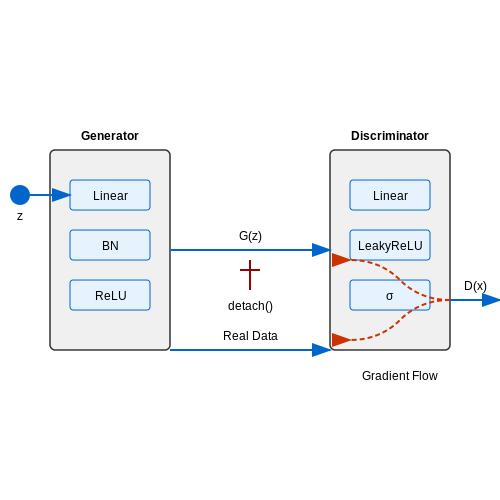
Initializing Weights for Stability
Weight initialization critically impacts the training dynamics of GANs, where improper scaling can lead to vanishing gradients, mode collapse, or unstable adversarial competition. The key challenge lies in maintaining balanced gradient flow through both the generator and discriminator during early training phases.
Xavier/Glorot Initialization
For linear layers with input dimension nin and output dimension nout, Xavier initialization draws weights from a uniform distribution:
This scaling preserves activation variances across layers when using sigmoid or tanh activations. In PyTorch, this is implemented as:
def init_weights(m):
    if isinstance(m, nn.Linear):
        nn.init.xavier_uniform_(m.weight)
        m.bias.data.fill_(0.01)

generator.apply(init_weights)
discriminator.apply(init_weights)
Kaiming/He Initialization
For ReLU-based networks, Kaiming initialization accounts for the zeroing-out of half the activations by using:
This variant is particularly effective for deep discriminators. The PyTorch implementation includes mode selection for leaky ReLU slopes:
nn.init.kaiming_normal_(m.weight, mode='fan_in', nonlinearity='leaky_relu')Orthogonal Initialization
Orthogonal initialization ensures weight matrices satisfy WTW = I, which helps prevent gradient covariance collapse in deep generators. The singular value decomposition (SVD)-based approach:
is implemented in PyTorch with gain scaling:
nn.init.orthogonal_(m.weight, gain=0.8)Layer-Specific Adaptations
Convolutional layers require special consideration due to their spatially local connectivity patterns. For transposed convolutions in generators, use fan-in scaling with 0.02 gain:
nn.init.normal_(m.weight, 0, 0.02)Batch normalization layers should initialize γ=1 and β=0 for stable gradient propagation, while zero-bias initialization in final discriminator layers prevents premature saturation.
5. Defining Loss Functions and Optimizers
5.1 Defining Loss Functions and Optimizers
The adversarial training process in GANs hinges on carefully designed loss functions and optimizers that drive the generator (G) and discriminator (D) toward equilibrium. The choice of loss function directly impacts training stability, convergence speed, and mode coverage.
Adversarial Loss Functions
The original GAN paper proposed a minimax game where D maximizes the probability of assigning correct labels to real and fake samples, while G minimizes the probability that D correctly identifies fakes. This translates to the following value function:
In practice, this formulation suffers from vanishing gradients early in training when D easily distinguishes real from fake samples. To address this, modern implementations often use the non-saturating loss, where G maximizes log(D(G(z))) instead of minimizing log(1 - D(G(z))):
Alternative Loss Formulations
Several improved loss variants have emerged to address training challenges:
- Wasserstein Loss: Uses Earth-Mover distance to provide meaningful gradients even when D achieves perfect separation. Requires Lipschitz constraint enforced via gradient penalty or weight clipping.
- Least Squares Loss: Replaces cross-entropy with squared errors to mitigate vanishing gradients and improve sample quality.
- Hinge Loss: Popular in BigGAN architectures, defined as max(0, 1 - D(x)) for real samples and max(0, 1 + D(G(z))) for fakes.
Optimizer Selection
The choice of optimizer significantly impacts GAN convergence. Key considerations include:
- Adam: Default choice with momentum terms (β₁=0.5, β₂=0.999) helps navigate complex loss landscapes. Learning rates typically range from 2e-4 to 1e-3.
- RMSProp: Effective for WGAN variants, particularly with gradient penalty.
- SGD with Nesterov Momentum: Sometimes preferred for its more predictable convergence in large-scale GANs.
Implementation in PyTorch
Below is a PyTorch implementation of the non-saturating loss with Adam optimizers:
# Initialize networks
generator = Generator()
discriminator = Discriminator()

# Define optimizers
g_optim = torch.optim.Adam(generator.parameters(),
                         lr=2e-4, betas=(0.5, 0.999))
d_optim = torch.optim.Adam(discriminator.parameters(),
                         lr=2e-4, betas=(0.5, 0.999))

# Loss function
criterion = torch.nn.BCELoss()

# Training loop
for real_data, _ in dataloader:
    # Train discriminator
    d_optim.zero_grad()

    # Real data loss
    real_pred = discriminator(real_data)
    real_loss = criterion(real_pred, torch.ones_like(real_pred))

    # Fake data loss
    noise = torch.randn(batch_size, latent_dim)
    fake_data = generator(noise)
    fake_pred = discriminator(fake_data.detach())
    fake_loss = criterion(fake_pred, torch.zeros_like(fake_pred))

    d_loss = real_loss + fake_loss
    d_loss.backward()
    d_optim.step()

    # Train generator
    g_optim.zero_grad()
    fake_pred = discriminator(fake_data)
    g_loss = criterion(fake_pred, torch.ones_like(fake_pred))
    g_loss.backward()
    g_optim.step()
Training Dynamics
The discriminator's loss should theoretically converge to log(4) ≈ 1.386 when p_data = p_g and D becomes optimal. In practice, monitor:
- Ratio of discriminator to generator updates (typically 1:1 or 5:1)
- Gradient norms to detect vanishing/exploding gradients
- Inception Score or FID for quantitative evaluation
5.2 Implementing the Training Loop
The training loop for a GAN involves alternating updates between the generator (G) and discriminator (D), each optimizing their respective loss functions. The discriminator aims to maximize the probability of correctly classifying real and fake samples, while the generator minimizes the discriminator's ability to distinguish its outputs from real data.
Discriminator Update
The discriminator's loss combines two terms: the negative log-likelihood for real data and the negative log-likelihood for generated data. For a batch of real samples x and noise vectors z, the loss is:
In practice, this translates to two forward passes through D: one for real data and one for generated data. The gradients are computed with respect to D's parameters and updated via backpropagation. Batch normalization or spectral normalization is often applied to stabilize training.
Generator Update
The generator's loss is designed to fool the discriminator. The original GAN paper proposes minimizing:
However, this formulation can lead to vanishing gradients early in training. A more stable alternative is to minimize:
Modern implementations often use the non-saturating loss, which provides stronger gradients when the generator performs poorly:
Training Dynamics
The training loop follows these steps:
- Sample a batch of real data x from the training set.
- Sample a batch of noise vectors z from the prior distribution (e.g., Gaussian).
- Generate fake samples G(z).
- Update the discriminator using both real and fake samples.
- Sample new noise vectors z'.
- Update the generator using the discriminator's responses to G(z').
This alternation continues until convergence, typically monitored via visual inspection of generated samples or quantitative metrics like Inception Score or Fréchet Inception Distance.
PyTorch Implementation
The core training loop in PyTorch involves:
for epoch in range(num_epochs):
    for real_data, _ in dataloader:
        # Update discriminator
        optimizer_D.zero_grad()
        z = torch.randn(batch_size, latent_dim)
        fake_data = generator(z)
        real_pred = discriminator(real_data)
        fake_pred = discriminator(fake_data.detach())
        loss_D = -torch.mean(torch.log(real_pred) + torch.log(1 - fake_pred))
        loss_D.backward()
        optimizer_D.step()

        # Update generator
        optimizer_G.zero_grad()
        z = torch.randn(batch_size, latent_dim)
        fake_data = generator(z)
        fake_pred = discriminator(fake_data)
        loss_G = -torch.mean(torch.log(fake_pred))
        loss_G.backward()
        optimizer_G.step()
Advanced Techniques
To improve stability, consider:
- Label smoothing: Replace hard 0/1 labels with smoothed values (e.g., 0.9/0.1) to prevent overconfident discriminator predictions.
- Gradient penalty: Used in Wasserstein GANs to enforce Lipschitz continuity via a regularization term on the discriminator's gradients.
- Two-time-scale update rule (TTUR): Use different learning rates for G and D to maintain equilibrium.
5.3 Monitoring Training Progress
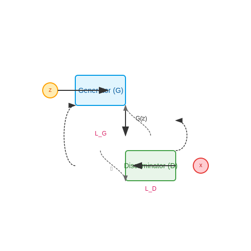
Monitoring the training progress of a GAN is critical due to its adversarial nature, where the generator and discriminator are in a dynamic equilibrium. Unlike traditional neural networks, GANs lack a single loss metric that reliably indicates convergence. Instead, multiple quantitative and qualitative techniques must be employed to assess training stability and output quality.
Loss Function Tracking
The discriminator loss LD and generator loss LG should be logged at each iteration. However, interpreting these values requires caution:
In practice, LD approaching zero indicates a failing generator, while LG decreasing while LD increases suggests mode collapse. Plotting these losses on a log scale helps identify trends that linear scales might obscure.
Inception Score and Fréchet Inception Distance
For image generation tasks, the Inception Score (IS) and Fréchet Inception Distance (FID) provide quantitative measures of sample quality and diversity:
Where μ and Σ are the mean and covariance of Inception-v3 features for real (r) and generated (g) samples. Lower FID and higher IS indicate better performance. These should be computed on a held-out validation set every k iterations.
Visual Inspection of Generated Samples
Periodically saving and inspecting generated samples provides immediate feedback on mode collapse, artifacts, or quality degradation. Implement a callback that saves a grid of generated images at regular intervals, using fixed noise vectors to track progression of specific outputs over time.
def save_sample_images(generator, epoch, fixed_noise, device):
    with torch.no_grad():
        fake = generator(fixed_noise.to(device)).cpu()
        grid = torchvision.utils.make_grid(fake, normalize=True)
        plt.imshow(grid.permute(1, 2, 0))
        plt.savefig(f'samples_epoch_{epoch}.png')
Gradient Norm Monitoring
Tracking the L2 norm of gradients for both networks helps diagnose vanishing or exploding gradients:
def log_gradient_norms(model):
    total_norm = 0
    for p in model.parameters():
        if p.grad is not None:
            param_norm = p.grad.data.norm(2)
            total_norm += param_norm.item()  2
    return total_norm  0.5
Sudden spikes or drops in gradient norms often precede training instability and should trigger learning rate adjustments or other interventions.
Discriminator Accuracy Metrics
Compute the discriminator's accuracy on both real and fake samples separately:
An ideal discriminator should maintain accuracy near 0.5 as training progresses, indicating equilibrium. Persistent high accuracy (>0.8) in either domain suggests an imbalance requiring architectural or hyperparameter adjustments.
6. Visualizing Generated Samples
6.1 Visualizing Generated Samples
Monitoring the progress of a GAN during training requires visualizing generated samples at regular intervals. Unlike discriminative models where loss metrics alone suffice, GANs demand qualitative assessment due to their adversarial nature. The generator's output must be inspected to detect mode collapse, artifacts, or convergence issues.
Tensor to Image Conversion
PyTorch stores images as tensors with shape (batch_size, channels, height, width) normalized to [-1, 1] or [0, 1]. To display these using Matplotlib, they must be:
- Converted to NumPy arrays via
.detach().cpu().numpy() - Reshaped to (height, width, channels) for RGB visualization
- Denormalized if necessary (e.g., scaling from [-1, 1] to [0, 255])
def tensor_to_image(tensor):
    # Move tensor to CPU and convert to NumPy
    image = tensor.detach().cpu().numpy()
    # Transpose from (C, H, W) to (H, W, C)
    image = image.transpose(1, 2, 0)
    # Denormalize from [-1, 1] to [0, 1]
    image = (image + 1) / 2.0
    # Clip values to ensure valid range
    image = np.clip(image, 0, 1)
    return image
Batch Visualization with Grid Layout
For batch processing, use torchvision.utils.make_grid to arrange samples in a grid before conversion. This function handles:
- Normalization scaling
- Padding between images
- Batch dimension flattening
import torchvision.utils as vutils

def visualize_batch(batch, nrow=8):
    # Create grid layout
    grid = vutils.make_grid(batch, nrow=nrow, normalize=True, padding=2)
    # Convert to plottable format
    grid_image = tensor_to_image(grid)
    # Display using Matplotlib
    plt.figure(figsize=(15, 15))
    plt.imshow(grid_image)
    plt.axis('off')
    plt.show()
Dynamic Training Monitoring
During training, periodically save generated samples to track evolution. Implement a callback that:
- Generates samples from fixed noise vectors (for consistent comparison)
- Logs images to TensorBoard or disk
- Applies post-processing like interpolation for latent space analysis
def generate_and_save_images(generator, epoch, fixed_noise):
    with torch.no_grad():
        fake_images = generator(fixed_noise).detach()

    fig = plt.figure(figsize=(10, 10))
    for i in range(fake_images.shape[0]):
        plt.subplot(4, 4, i+1)
        plt.imshow(tensor_to_image(fake_images[i]))
        plt.axis('off')

    plt.savefig(f'gan_samples_epoch_{epoch}.png')
    plt.close()
Quantitative Metrics Integration
Combine visualization with metrics like Inception Score (IS) or Fréchet Inception Distance (FID):
where μ and Σ are the mean and covariance of real (r) and generated (g) features extracted from a pretrained Inception-v3 network.
6.2 Quantitative Evaluation Metrics
Evaluating GANs quantitatively remains challenging due to the lack of a definitive metric that captures both sample quality and diversity. Unlike discriminative models, where metrics like accuracy or F1-score suffice, GANs require specialized evaluation techniques. Three widely adopted metrics are the Inception Score (IS), Fréchet Inception Distance (FID), and Precision-Recall for Distributions (PRD).
Inception Score (IS)
The Inception Score measures both the quality and diversity of generated samples by leveraging a pre-trained Inception-v3 model. It computes the KL divergence between the conditional class distribution p(y|x) and the marginal class distribution p(y):
Higher IS values indicate better performance, as they imply the model generates meaningful and diverse samples. However, IS has limitations—it relies heavily on the Inception-v3 model's biases and fails to detect mode collapse if the generated distribution has high entropy.
Fréchet Inception Distance (FID)
FID addresses some shortcomings of IS by comparing the statistics of real and generated samples in the feature space of Inception-v3. Given real samples X and generated samples Y, their feature distributions are modeled as multivariate Gaussians N(μ_X, Σ_X) and N(μ_Y, Σ_Y). The FID is computed as:
Lower FID values indicate better alignment between real and generated distributions. Unlike IS, FID is sensitive to mode collapse and provides a more robust measure of sample quality.
Precision-Recall for Distributions (PRD)
PRD evaluates GANs by decomposing the evaluation into precision (quality) and recall (diversity). Given real distribution P and generated distribution Q, precision measures the fraction of Q that lies within the support of P, while recall measures the fraction of P covered by Q. The PRD curve is defined as:
where λ is a trade-off parameter. PRD provides a more nuanced evaluation than IS or FID, particularly in detecting partial mode collapse.
Implementation in PyTorch
Below is a PyTorch implementation for computing FID, adapted from the pytorch-fid library:
import torch
import numpy as np
from scipy.linalg import sqrtm

def calculate_fid(real_features, gen_features):
    mu_real, sigma_real = torch.mean(real_features, dim=0), torch_cov(real_features)
    mu_gen, sigma_gen = torch.mean(gen_features, dim=0), torch_cov(gen_features)

    diff = mu_real - mu_gen
    covmean = sqrtm(sigma_real @ sigma_gen)
    fid = diff.dot(diff) + torch.trace(sigma_real + sigma_gen - 2 * covmean)
    return fid.item()

def torch_cov(m, rowvar=False):
    if m.dim() > 2:
        raise ValueError('Input must be 2D')
    m = m if rowvar else m.t()
    fact = 1.0 / (m.size(1) - 1)
    m_centered = m - torch.mean(m, dim=1, keepdim=True)
    return fact * m_centered @ m_centered.t()
For IS and PRD, existing libraries like torch-fidelity or gan-metrics provide optimized implementations. When evaluating GANs, it is advisable to report multiple metrics to capture different aspects of performance.
6.3 Common Pitfalls and How to Avoid Them
Mode Collapse
Mode collapse occurs when the generator produces a limited variety of samples, often converging to a few modes or even a single mode of the data distribution. This happens because the discriminator fails to provide meaningful gradients, allowing the generator to exploit a narrow set of features that consistently fool the discriminator. Mathematically, this can be understood as the generator optimizing for a subset of the data distribution:
To mitigate mode collapse:
- Use mini-batch discrimination: This technique allows the discriminator to compare multiple samples in a batch, making it harder for the generator to produce identical outputs.
- Implement unrolled GANs: By unrolling the optimization steps of the discriminator, the generator receives more stable gradients.
- Apply diversity-promoting losses: Techniques like feature matching or adding entropy regularization encourage the generator to explore more modes.
Vanishing Gradients
When the discriminator becomes too strong, the generator's gradients can vanish, halting training. This is particularly problematic early in training when the generator's outputs are easily distinguishable from real data. The gradient of the generator's loss with respect to its parameters can become negligible:
Solutions include:
- Modify the generator's loss function: Instead of minimizing \(\log(1 - D(G(z)))\), maximize \(\log D(G(z))\) to provide stronger gradients.
- Use Wasserstein GAN (WGAN): The Wasserstein distance provides more stable gradients by avoiding saturation in the discriminator's outputs.
- Balance training: Ensure the discriminator does not overpower the generator by adjusting their learning rates or training frequencies.
Oscillations and Instability
GAN training often exhibits oscillatory behavior, where the generator and discriminator continuously undo each other's progress. This instability arises from the adversarial nature of the training process, where the Nash equilibrium is hard to achieve. The dynamics can be visualized as a non-converging game between two players.
Strategies to stabilize training:
- Use spectral normalization: This constrains the Lipschitz constant of the discriminator, preventing overly large weight updates.
- Apply gradient penalty: As in WGAN-GP, penalizing the gradient norm of the discriminator helps maintain stable training dynamics.
- Optimize with adaptive methods: Techniques like Adam or RMSprop can help smooth out oscillations by adapting learning rates dynamically.
Hyperparameter Sensitivity
GANs are notoriously sensitive to hyperparameters, including learning rates, batch sizes, and network architectures. Small changes can lead to drastically different outcomes, making reproducibility challenging.
Best practices:
- Grid search for critical parameters: Systematically explore learning rates and architecture choices to find stable configurations.
- Monitor training dynamics: Track metrics like discriminator accuracy, generator loss, and sample diversity to detect issues early.
- Use progressive growing: Start with low-resolution images and gradually increase complexity to ease the optimization process.
Evaluation Challenges
Unlike supervised learning, GANs lack a straightforward metric to evaluate performance. Common pitfalls include relying solely on visual inspection or using inappropriate metrics like Inception Score (IS) or Fréchet Inception Distance (FID) without understanding their limitations.
Robust evaluation strategies:
- Combine multiple metrics: Use both FID and precision/recall for generative models to capture different aspects of performance.
- Track training curves: Monitor discriminator and generator losses over time to identify divergence or saturation.
- Conduct human evaluation: Supplement quantitative metrics with qualitative assessments to ensure sample quality aligns with expectations.
7. Key Research Papers on GANs
7.1 Key Research Papers on GANs
- (PDF) Must-Read Papers on GANs - Academia.edu — The research study examines current advancements in GANs, including self-attention, adversarial autoencoders, and attention mechanisms. Additionally, the paper addresses the ethical issues related to GANs, such as the possible exploitation of data created by GANs and bias in training data.
- Diffusion-GAN — Official PyTorch implementation - GitHub — Here, we explain how to train general GANs with diffusion. We provide two ways: a. plug-in as simple as a data augmentation method; b. training GANs on diffusion chains with a timestep-dependent discriminator. Currently, we didn't find significant empirical differences of the two approaches, while the second approach has stronger theoretical guarantees. We suspect when advanced timestep ...
- Understanding GANs: fundamentals, variants, training challenges ... — Generative adversarial networks (GANs), a novel framework for training generative models in an adversarial setup, have attracted significant attention in recent years. The two opposing neural networks of the GANs framework, i.e., a generator and a discriminator, are trained simultaneously in a zero-sum game, where the generator generates images to fool the discriminator that is trained to ...
- Generative Adversarial Networks: Applications, Challenges, and Open ... — Generative Adversarial Networks (GANs) represent an emerging class of deep generative models that have been attracting notable interest in recent years. These networks are unique in their capacity to train high-dimensional distributions spanning a range of data types. Conventional GANs encounter problems related to model collapse, convergence, and instability. These issues can be primarily ...
- Artificial Intelligence - Part 7.1 - GENERATIVE AI - GANs - LinkedIn — This expanded article delves into the intricacies of GANs, including their mechanisms, training process, implementation, advanced concepts, and challenges, alongside real-world examples and ...
- GitHub - Pushkar-v/Generating-Synthetic-Data-using-GANs: Generating ... — The Proposed solution by the team involves generating Synthetic Data using Generative Adversarial Networks or GANs and with the help of conventionally available sources such as TGAN and CTGAN. The team also wants to build modules which can test the generated synthetic data against the original datasets on following three areas: Statistical Similarity: Create standardized modules to check if ...
- GAN (Generative Adversarial Network) - KiKaBeN — In this article, I'll explain how GAN (Generative Adversarial Network) works while implementing it step-by-step with PyTorch. GAN is a generative model that produces random images given a random input. We will define the model and train it. 1 Introduction 1.1 Ian Goodfellow and GAN As you probably know, Ian Goodfellow proposed GAN in 2014. I believe many people think of GAN when they think ...
- A survey on GANs for computer vision: Recent research, analysis and ... — This research approach tries to enhance the similarity between original and synthesized data distributions by defining an appropriate loss function. Surveys such as [34] are focus on analyzing the state-of-the-art GANs and further analyzing the performance of a huge variety of networks.
- GitHub - tkarras/progressive_growing_of_gans: Progressive Growing of ... — Progressive Growing of GANs for Improved Quality, Stability, and Variation — Official TensorFlow implementation of the ICLR 2018 paper
- (PDF) Generative Adversarial Networks: Applications, Challenges, and ... — PDF | Generative Adversarial Networks (GANs) represent an emerging class of deep generative models that have been attracting notable interest in recent... | Find, read and cite all the research ...
7.2 Advanced PyTorch Tutorials
- Gans In Action: Deep Learning With Generative Adversarial ... - Library — GANs in action Now that you have a high-level understanding of GANs and their constituent networks, let's take a closer look at the system in action. Imagine that our goal is to teach a GAN to produce realistic-looking handwritten digits. (You'll learn to implement GANs in action 7 such a model in chapter 3 and expand on it in chapter 4.)
- Deep Learning with Pytorch - PDFCOFFEE.COM — PyTorch derives a significant part of its codebase from the Torch7 project started in 2007 by Ronan Collobert and others, which has roots in the Lush programming language pioneered by Yann LeCun and Leon Bottou. This rich history helped us focus on what needed to change, rather than conceptually starting from scratch.
- Advanced: Making Dynamic Decisions and the Bi-LSTM CRF - PyTorch — Pytorch is a dynamic neural network kit. Another example of a dynamic kit is Dynet (I mention this because working with Pytorch and Dynet is similar. If you see an example in Dynet, it will probably help you implement it in Pytorch). The opposite is the static tool kit, which includes Theano, Keras, TensorFlow, etc. The core difference is the ...
- D2L - Dive into Deep Learning — Dive into Deep Learning 1.0.3 ... — Implemented with PyTorch, NumPy/MXNet, JAX, and TensorFlow Adopted at 500 universities from 70 countries Star. ... Center for Research and Advanced Studies of the National Polytechnic Institute ... Recurrent Neural Network Implementation from Scratch; 9.6. Concise Implementation of Recurrent Neural Networks; 9.7. Backpropagation Through Time;
- GitHub - ozanciga/gans-with-pytorch: Various implementations of ... — I started doing this work with Pytorch 0.4.0 and Python 3.6 (with Cuda 9.0 and CuDNN 7), with Ubuntu 16.04. Around right after "SRGAN"s, I switched to Pytorch 0.4.1, Cuda 9.2 and CuDNN 7.2. For visualizing the GAN generation progress on your browser, you will need the facebook's visdom library.
- d2l en | PDF | Deep Learning | Artificial Intelligence - Scribd — This document is a book about deep learning. It introduces deep learning concepts and provides tutorials on how to implement various deep learning models like convolutional neural networks, recurrent neural networks, and more using MXNet. The book begins with the basics of deep learning and progresses to more advanced topics. It includes code examples and explanations to help readers learn and ...
- PyTorch for Data Scientists: Machine Learning and Deep Learning with ... — Read online or download for free from Z-Library the Book: PyTorch for Data Scientists: Machine Learning and Deep Learning with Python, Author: Barry Luiz, Publisher ...
- Deep Learning For Computer Vision With Python [PDF] [46lb33513le0] — 7.2.3 Implementing k-NN The goal of this section is to train a k-NN classifier on the raw pixel intensities of the Animals dataset and use it to classify unknown animal images. We'll be using our four step pipeline to train classifiers from Section 4.3.2: • Step #1 - Gather Our Dataset: The Animals datasets consists of 3,000 images with ...
- Intro to Generative Adversarial Networks (GANs) — Training GANs The Minimax game: G vs. D. Most deep learning models (for example, image classification) are based on optimization: finding the low value of the cost function. GANs are different because the two networks: the generator and discriminator, each has its own cost with opposite objectives:
- PDF Neural Networks And Deep Learning A Textbook - www.blog.orats — Neural Networks And Deep Learning A Textbook Deep LearningDeep LearningPractical Deep LearningDeep Learning for Coders with Fastai & PyTorchIntroduction to Deep LearningLearning Deep
7.3 Community Resources and Forums
- Understanding GANs: fundamentals, variants, training challenges ... — Generative adversarial networks (GANs), a novel framework for training generative models in an adversarial setup, have attracted significant attention in recent years. The two opposing neural networks of the GANs framework, i.e., a generator and a discriminator, are trained simultaneously in a zero-sum game, where the generator generates images to fool the discriminator that is trained to ...
- Building a GAN (Generative Adversarial Network) - Lightning AI — We will train it with PyTorch Lightning and make a simple dashboard with Gradio, using the beautiful and seamless integration provided by the Lightning framework. To start, we need to install Lightning, but first, I will create and activate a new Python 3.8 environment for my new app. Check out this Lightning Bits episode to learn more about ...
- GAN (Generative Adversarial Network) - KiKaBeN — In this article, I'll explain how GAN (Generative Adversarial Network) works while implementing it step-by-step with PyTorch. GAN is a generative model that produces random images given a random input. We will define the model and train it. 1 Introduction 1.1 Ian Goodfellow and GAN. As you probably know, Ian Goodfellow proposed GAN in 2014. I ...
- PyTorch — Join PyTorch Foundation As a member of the PyTorch Foundation, you'll have access to resources that allow you to be stewards of stable, secure, and long-lasting codebases. You can collaborate on training, local and regional events, open-source developer tooling, academic research, and guides to help new users and contributors have a ...
- Get Started - PyTorch — To install PyTorch via pip, and do have a ROCm-capable system, in the above selector, choose OS: Linux, Package: Pip, Language: Python and the ROCm version supported. Then, run the command that is presented to you. Verification. To ensure that PyTorch was installed correctly, we can verify the installation by running sample PyTorch code.
- Generative Adversarial Networks: Applications, Challenges, and Open ... — Generative Adversarial Networks (GANs) represent an emerging class of deep generative models that have been attracting notable interest in recent years. These networks are unique in their capacity to train high-dimensional distributions spanning a range of data types. Conventional GANs encounter problems related to model collapse, convergence, and instability. These issues can be primarily ...
- Gans In Action: Deep Learning With Generative Adversarial ... - Library — Other online resources GANs are an active field with excellent (albeit fragmented) resources only a Google search away. Those with an academic bent can find the latest papers in arXiv (https:// arxiv.org), an online repository of academic e-prints owned and operated by Cornell University.
- Generative adversarial network - Wikipedia — A generative adversarial network (GAN) is a class of machine learning frameworks and a prominent framework for approaching generative artificial intelligence.The concept was initially developed by Ian Goodfellow and his colleagues in June 2014. [1] In a GAN, two neural networks compete with each other in the form of a zero-sum game, where one agent's gain is another agent's loss.
- How to Develop a Wasserstein Generative Adversarial Network (WGAN) From ... — The Wasserstein Generative Adversarial Network, or Wasserstein GAN, is an extension to the generative adversarial network that both improves the stability when training the model and provides a loss function that correlates with the quality of generated images. The development of the WGAN has a dense mathematical motivation, although in practice requires only a few minor modifications to the ...
- Some notes on generating software synthesizer patches with AI — Some notes on generating software synthesizer patches with AI - generating-synth-patches-with-ai.md