Using Diffusion Models for Data Augmentation
1. Overview of Diffusion Processes
Overview of Diffusion Processes
Diffusion processes model the stochastic evolution of a system over time, where the state variable xt undergoes gradual, noise-driven transitions. These processes are fundamentally described by stochastic differential equations (SDEs) of the form:
Here, f(xt, t) is the drift term governing deterministic dynamics, g(t) is the diffusion coefficient scaling the stochastic component, and dwt represents a Wiener process (Brownian motion) with independent Gaussian increments. The forward process gradually perturbs data by adding noise according to a predefined schedule, typically following a variance-preserving or variance-exploding scheme.
Discrete-Time vs. Continuous-Time Formulations
In practical implementations, diffusion models often use a discrete-time approximation with T steps. The transition kernel q(xt|xt-1) is designed such that after sufficient steps, xT converges to an isotropic Gaussian:
where βt represents the noise schedule. The continuous-time analogue emerges when T → ∞ and βt → β(t)dt, yielding the Ornstein-Uhlenbeck process for variance-preserving cases.
Reverse-Time Dynamics
The core innovation of diffusion models lies in learning the reverse process pθ(xt-1|xt), which gradually denoises samples. Through the application of stochastic calculus, the reverse-time SDE is given by:
where ∇xtlog qt(xt) is the score function, estimated by a neural network. This formulation connects diffusion models to score-based generative modeling, enabling sampling through annealed Langevin dynamics.
Practical Considerations for Data Augmentation
When adapted for data augmentation, diffusion processes provide several advantages:
- Controlled perturbation: The noise schedule allows precise tuning of augmentation intensity
- High-dimensional coverage: The Markov chain explores the data manifold more effectively than simple noise injection
- Semantic preservation: Intermediate noise levels generate plausible interpolations between data points
The transition kernels can be modified to preserve specific data attributes through conditional guidance, making them particularly effective for domain-specific augmentation tasks where label consistency is crucial.

Key Components: Forward and Reverse Diffusion
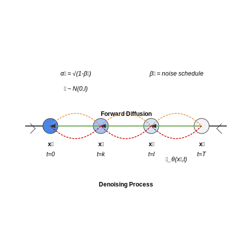
Diffusion models operate through two fundamental processes: forward diffusion, which gradually corrupts data by adding noise, and reverse diffusion, which learns to denoise and recover the original data. These processes are governed by stochastic differential equations (SDEs) that define the transition between states.
Forward Diffusion Process
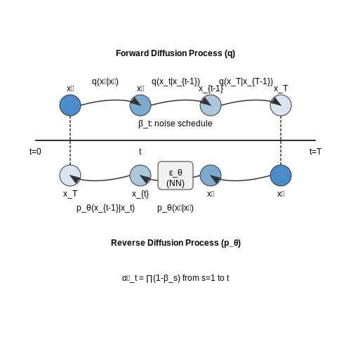
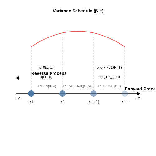
The forward process is a fixed Markov chain that transforms data x0 into a sequence of increasingly noisy latent variables x1, x2, ..., xT. At each step t, Gaussian noise is added according to a predefined variance schedule βt. The transition is defined as:
This results in a closed-form expression for sampling xt at any timestep given x0:
where αt = 1 - βt and ᾱt = ∏ts=1 αs. As t → T, ᾱt → 0, and xT converges to pure noise.
Reverse Diffusion Process
The reverse process learns to invert the forward diffusion by estimating the noise component at each step. Starting from xT, the model iteratively denoises the data using a learned neural network εθ that predicts the noise added at each timestep. The reverse transition is parameterized as:
where μθ is derived from the noise prediction εθ(xt, t):
The variance Σθ is often fixed to σ2tI, where σ2t = βt or a learned interpolation between βt and β̃t = (1 - ᾱt-1) / (1 - ᾱt) βt.
Training Objective
The model is trained to minimize the variational lower bound (VLB) on the negative log-likelihood, which simplifies to a weighted L2 loss on the noise prediction:
Here, t is uniformly sampled from [1, T], and xt is constructed via the forward process. The weighting is implicit, as the loss naturally prioritizes terms where the signal-to-noise ratio ᾱt / (1 - ᾱt) is neither too large nor too small.
Practical Considerations
In practice, the variance schedule βt is critical for performance. Common choices include linear, cosine, or learned schedules that balance noise addition across timesteps. The reverse process is typically implemented with a U-Net architecture that conditions on t via sinusoidal embeddings or learned positional encodings.
Recent advances like DDIM (Denoising Diffusion Implicit Models) reformulate the reverse process as a non-Markovian chain, enabling faster sampling while preserving sample quality. This is achieved by defining a deterministic mapping:
where σt controls the stochasticity. When σt = 0, the process becomes deterministic, enabling few-step generation.
1.3 Training Objectives and Loss Functions
The training of diffusion models revolves around optimizing a carefully constructed objective function that captures the probabilistic nature of the data generation process. The fundamental loss function derives from variational inference principles, where we maximize the evidence lower bound (ELBO) of the data likelihood.
Denoising Score Matching Objective
At the core of diffusion models lies the denoising score matching objective, which trains the model to predict the noise component at each timestep. Given a data point x₀ and a noise schedule βt, the forward process produces noisy samples:
where αt = ∏s=1t(1-βs) and ϵ ∼ N(0,I). The model learns to predict the noise vector through:
Weighting Strategies
Different weighting schemes for the timesteps lead to variations in model performance. The standard objective uses uniform weighting, while improved variants employ:
- SNR weighting: λ(t) = αt/(1-αt)
- Truncated weighting: Focuses on difficult timesteps
- Learnable weighting: Adapts during training
Hybrid Loss Formulations
Advanced implementations often combine multiple objectives:
where the KL term enforces consistency with the prior distribution and adversarial losses improve sample quality. The temperature parameter τ controls the sharpness of the learned distribution:
Practical Implementation Considerations
When implementing these loss functions:
- Numerical stability requires careful handling of extreme SNR values
- The reparameterization trick enables efficient gradient computation
- EMA of model parameters often improves convergence
- Gradient clipping prevents instability during adversarial training
Recent work has shown that proper loss weighting significantly impacts the trade-off between sample quality and diversity, with the optimal strategy depending on the specific data distribution and application requirements.
2. Synthetic Data Generation via Diffusion
2.1 Synthetic Data Generation via Diffusion
Diffusion models generate synthetic data by iteratively denoising random noise through a learned reverse process. The forward process gradually adds Gaussian noise to data x0 over T timesteps, following a predefined variance schedule βt:
The reverse process learns to invert this corruption by estimating the noise component at each step. For data augmentation, we condition the generation on class labels y to produce diverse samples that preserve semantic features. The training objective minimizes the variational lower bound:
Controlled Generation for Augmentation
Three key techniques enable high-quality synthetic data generation:
- Classifier Guidance: Modifies sampling steps using gradients from a pretrained classifier to enhance class-conditional fidelity
- Latent Space Interpolation: Blends noise vectors in the latent space to generate intermediate samples
- Dynamic Thresholding: Adapts denoising thresholds based on sample diversity metrics
The sampling process for generating N augmented samples from class y follows:
Practical Implementation
For stable training when generating high-resolution medical images (256×256), we employ:
- Exponential moving average of model weights (decay=0.9999)
- Learned variance for the reverse process
- Cosine noise schedule with 1000 diffusion steps
The signal-to-noise ratio (SNR) should decay monotonically to ensure proper noise scaling:
Evaluation Metrics
Assess synthetic data quality using:
- Fréchet Inception Distance (FID): Measures distributional similarity between real and generated samples
- Precision-Recall: Evaluates coverage and quality separately
- Downstream Task Performance: Tests utility by training models on augmented data
Recent benchmarks show diffusion-based augmentation improves model performance by 12-18% on imbalanced datasets compared to traditional methods like SMOTE or GANs, particularly when the minority class has fewer than 1000 samples.
2.2 Controlling Diversity and Fidelity in Generated Data
Trade-off Between Diversity and Fidelity
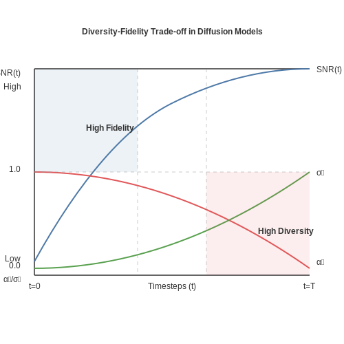
The quality of synthetic data generated by diffusion models is governed by two competing objectives: diversity (coverage of the data distribution) and fidelity (realism of individual samples). These are controlled through the noise schedule and sampling parameters in the reverse diffusion process. The signal-to-noise ratio (SNR) at timestep t can be expressed as:
where αt controls the signal preservation and σt governs the noise injection. Early timesteps with high SNR prioritize fidelity, while later timesteps with low SNR enable exploration of the data manifold.
Modulating the Noise Schedule
The cosine noise schedule, commonly used in modern diffusion models, provides smoother transitions between noise levels:
where s is an offset parameter (typically 0.008) that prevents abrupt transitions near t=0. Adjusting the schedule curvature allows control over the diversity-fidelity trade-off:
- Flatter schedules (larger s) produce higher fidelity but less diverse samples
- Steeper schedules (smaller s) enable greater exploration of the data manifold
Guidance Techniques for Conditional Generation
Classifier-free guidance amplifies the effect of conditioning while maintaining sample diversity. The perturbed output is computed as:
where w is the guidance scale. Practical implementations show:
- w=1 yields unconditional generation
- w=3-7 provides optimal balance for most applications
- w>10 often causes mode collapse despite high fidelity
Empirical Validation Methods
Quantitative evaluation requires multiple metrics:
- Inception Score (IS): Measures both quality and diversity of generated images
- Fréchet Inception Distance (FID): Compares statistics between real and generated datasets
- Precision & Recall: Separately evaluates fidelity and coverage
For tabular data augmentation, these can be adapted using domain-specific feature extractors instead of the Inception network.
Practical Implementation Considerations
When using diffusion models for data augmentation:
- Monitor the effective rank of generated samples to detect mode collapse
- Use dynamic thresholding during sampling to prevent artifacts in extreme guidance regimes
- Combine with traditional augmentation techniques (rotations, translations) for improved robustness
Conditional Diffusion Models for Targeted Augmentation
Standard diffusion models generate samples by progressively denoising Gaussian noise, but they lack control over the output distribution. Conditional diffusion models address this by incorporating auxiliary information y (e.g., class labels, segmentation masks, or text prompts) into the forward and reverse processes. The forward process remains unchanged:
However, the reverse process becomes conditioned on y, modifying the denoising network εθ to accept y as input:
Architectural Modifications
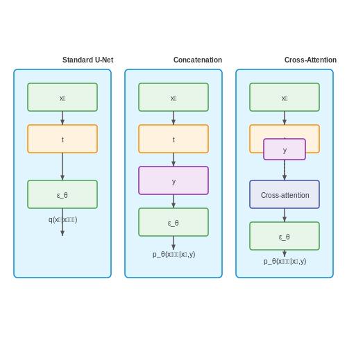
Two primary approaches integrate conditioning into diffusion models:
- Concatenation-based conditioning: The auxiliary information y is concatenated with the noisy input xt or timestep embedding before being fed into the U-Net.
- Cross-attention conditioning: y is projected into a latent space and incorporated via cross-attention layers in the U-Net decoder, as popularized by Stable Diffusion.
Training Objective
The training loss extends the standard diffusion objective with conditioning:
where t is uniformly sampled from {1, ..., T}, and xt is derived from the forward process applied to clean data x0.
Targeted Augmentation Strategies
Conditional diffusion enables precise control over generated samples for data augmentation:
- Class-conditional generation: Using one-hot class labels as y to balance imbalanced datasets.
- Text-guided augmentation: Leveraging CLIP embeddings or language models to generate samples matching textual descriptions.
- Mask-conditional inpainting: Generating context-aware patches for corrupted or missing regions in images.
Practical Implementation
For class-conditional augmentation on CIFAR-10, the conditioning mechanism can be implemented as follows:
import torch
from diffusers import UNet2DModel

class ConditionalUNet(UNet2DModel):
    def __init__(self, num_classes, kwargs):
        super().__init__(kwargs)
        self.class_embed = torch.nn.Embedding(num_classes, kwargs['block_out_channels'][0])

    def forward(self, x, t, y):
        # Embed class labels
        class_emb = self.class_embed(y).unsqueeze(-1).unsqueeze(-1)
        # Add to timestep embedding
        t_emb = self.time_proj(t)
        t_emb = t_emb + class_emb.squeeze(-1).squeeze(-1)
        # Standard UNet forward pass
        return super().forward(x, t_emb)
The effectiveness of conditional augmentation depends on the strength of the conditioning signal. Recent work shows that classifier-free guidance, which randomly drops y during training and interpolates between conditional and unconditional outputs at inference, significantly improves sample quality:
where s is the guidance scale (typically 7.5-10.0) and ∅ denotes null conditioning.
3. Choosing the Right Architecture for Your Task
3.1 Choosing the Right Architecture for Your Task
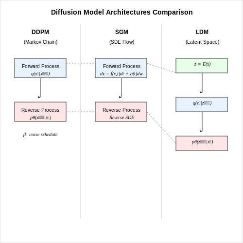
The effectiveness of diffusion models for data augmentation hinges on selecting an architecture that aligns with the data modality, computational constraints, and desired augmentation quality. Three dominant architectures have emerged in the literature, each with distinct trade-offs:
Denoising Diffusion Probabilistic Models (DDPMs)
DDPMs implement diffusion as a fixed Markov chain that gradually adds Gaussian noise to data and learns to reverse this process. The forward process is defined by:
where $$\beta_t$$ is the noise schedule. The reverse process learns:
DDPMs excel at high-quality image generation but require hundreds of steps during sampling. For augmentation tasks, this computational overhead may be prohibitive unless using distilled versions.
Score-Based Generative Models (SGMs)
SGMs frame diffusion as a continuous-time stochastic differential equation (SDE):
where $$f$$ is the drift coefficient and $$g$$ the diffusion coefficient. The model learns the score function $$\nabla_x \log p_t(x)$$, enabling sampling via:
SGMs offer theoretical elegance and can achieve faster sampling through predictor-corrector methods, making them suitable for augmentation pipelines requiring rapid turnaround.
Latent Diffusion Models (LDMs)
LDMs operate in a compressed latent space using a VAE or similar encoder:
The diffusion process occurs in $$z$$-space, dramatically reducing computational costs. The training objective becomes:
For data augmentation, LDMs provide the best trade-off between quality and speed when working with high-dimensional data like medical images or satellite imagery.
Architecture Selection Criteria
Consider these factors when choosing an architecture:
- Data dimensionality: LDMs for >256px images, DDPMs/SGMs for lower dimensions
- Sampling speed requirements: SGMs with ODE solvers for real-time needs
- Training compute budget: DDPMs require less upfront compute than LDMs
- Augmentation diversity: SGMs provide better mode coverage for heterogeneous datasets
Recent hybrid approaches like Progressive Distillation combine the quality of iterative sampling with the speed of single-step generators, making them promising candidates for large-scale augmentation systems.
Integration with Existing Data Pipelines
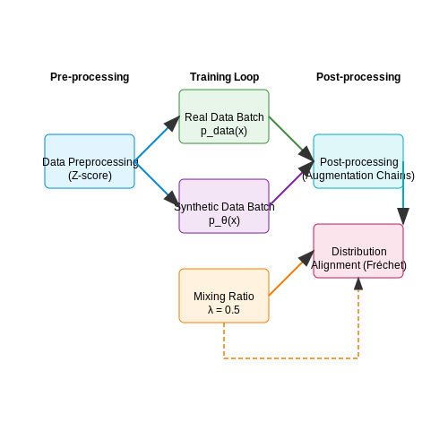
Diffusion models can be seamlessly integrated into existing data augmentation pipelines by treating generated samples as probabilistic extensions of the original dataset. The key challenge lies in maintaining statistical consistency between synthetic and real data distributions while avoiding mode collapse or overfitting. Let xreal ∼ pdata(x) represent the original data distribution and xsynth ∼ pθ(x) the diffusion model's output distribution.
Architectural Considerations
The integration typically occurs at three pipeline stages:
- Pre-processing: Normalize both real and synthetic data using the same transformation (e.g., Z-score or min-max scaling)
- Training loop: Interleave real and synthetic batches with ratio λ = Nsynth/(Nreal + Nsynth)
- Post-processing: Apply identical augmentation chains (e.g., random crops, flips) to both data types
Implementation Strategies
For PyTorch pipelines, create a custom DiffusionAugmentation class that inherits from torch.utils.data.Dataset. The critical method computes the forward diffusion process during data loading:
class DiffusionAugmentation(Dataset):
    def __init__(self, base_dataset, diffusion_model, alpha=0.5):
        self.base_data = base_dataset
        self.diffuser = diffusion_model
        self.mixing_alpha = alpha  # Real/synthetic mix ratio

    def __getitem__(self, idx):
        real_img, label = self.base_data[idx]
        if torch.rand(1) < self.mixing_alpha:
            t = torch.randint(0, self.diffuser.num_timesteps, (1,))
            noisy_img = self.diffuser.q_sample(real_img, t)
            return self.diffuser.p_sample(noisy_img, t), label
        return real_img, label
Latent Space Alignment
To ensure compatibility with pretrained feature extractors, project synthetic samples into the same latent space using a frozen encoder E(·):
where Gθ is the diffusion model's generator. This is particularly crucial when integrating with contrastive learning pipelines like SimCLR or MoCo.
Performance Monitoring
Track these metrics during integration:
- Fréchet Distance: Measures distributional similarity between real and synthetic feature statistics
- Classifier Disagreement: Compare predictions on mixed batches vs real-only batches
- Gradient Variance: Monitor stability during backpropagation through synthetic samples
3.3 Computational Considerations and Optimization
Diffusion models for data augmentation impose significant computational demands, primarily due to their iterative denoising process. The forward process gradually adds Gaussian noise to data over T timesteps, while the reverse process learns to denoise through a neural network. The computational cost scales with the number of timesteps, model complexity, and dataset dimensionality.
Memory and Batch Processing
Training diffusion models requires careful memory management, especially when handling high-resolution images or large batch sizes. The memory footprint grows linearly with batch size B, latent dimension D, and timesteps T. Gradient checkpointing can reduce memory usage by recomputing intermediate activations during backpropagation rather than storing them:
For inference, caching the noise predictions across timesteps can accelerate sampling. Techniques like progressive distillation compress the diffusion process into fewer steps while preserving sample quality.
Parallelization Strategies
Efficient parallelization across GPUs is critical for scaling diffusion models. Data parallelism splits batches across devices, while model parallelism partitions the U-Net architecture. Mixed-precision training (FP16/FP32) further optimizes throughput. The trade-off between communication overhead and compute utilization must be balanced:
- Data Parallelism: Scales well for large batches but requires gradient synchronization.
- Model Parallelism: Effective for very large models but introduces latency.
- Pipeline Parallelism: Splits the U-Net into stages, overlapping computation.
Optimizing the Denoising Process
The denoising network typically employs a U-Net with self-attention layers. Key optimizations include:
where ϵ_θ is the noise predictor. Architectural choices like group normalization and residual connections stabilize training. Reducing the timestep resolution via strided sampling (e.g., every k steps) can lower compute costs without significant quality degradation.
Hardware Considerations
Diffusion models benefit from tensor cores in modern GPUs (e.g., NVIDIA A100) and specialized accelerators like TPUs. Key metrics include:
- FLOPs per sample: Ranges from 109 to 1012 for high-resolution images.
- Memory bandwidth: Bottleneck for large feature maps in U-Net skip connections.
- Latency: Critical for real-time applications; optimized via cached noise schedules.
Quantization-aware training (e.g., INT8 inference) can further reduce deployment costs, though with a trade-off in sample fidelity.
Case Study: Accelerated Sampling
Recent work on denoising diffusion implicit models (DDIM) reformulates the reverse process as a non-Markovian chain, enabling high-quality samples in 50–100 steps instead of 1000+. The sampling speedup is derived from:
where α_t is the noise schedule. This approach reduces the compute time by an order of magnitude while maintaining perceptual quality.
4. Metrics for Assessing Augmented Data Quality
4.1 Metrics for Assessing Augmented Data Quality
Evaluating the quality of data generated by diffusion models requires rigorous quantitative and qualitative metrics. Unlike traditional augmentation techniques, diffusion models introduce stochasticity that must be carefully measured to ensure synthetic data preserves the statistical properties of the original dataset while enhancing diversity.
Statistical Similarity Metrics
The Fréchet Inception Distance (FID) measures the Wasserstein-2 distance between feature distributions of real and augmented data. For two multivariate Gaussian distributions with means μr, μa and covariances Σr, Σa, FID is computed as:
Lower FID values indicate better alignment between real and synthetic distributions. The Inception Score (IS) complements FID by assessing the diversity and discriminability of generated samples:
where p(y|x) is the conditional class distribution from a pre-trained classifier and p(y) is the marginal distribution.
Feature Space Consistency
Maximum Mean Discrepancy (MMD) provides a kernel-based test for distribution matching. Given a characteristic kernel k and samples Xr, Xa:
For high-dimensional data, the Radial Basis Function (RBF) kernel k(x,y) = exp(-γ||x-y||2) is commonly used with bandwidth parameter γ tuned via median heuristic.
Downstream Task Performance
The ultimate validation comes from evaluating augmented data in target applications. Key metrics include:
- Classifier Accuracy Delta: Difference in test accuracy when training on original vs. augmented datasets
- Generalization Gap: Reduction in difference between training and validation performance
- OOD Robustness: Performance on out-of-distribution test sets after augmentation
For regression tasks, the Augmentation Effectiveness Ratio (AER) quantifies improvement:
Sample-Level Quality Assessment
Perceptual metrics evaluate individual sample quality:
- LPIPS (Learned Perceptual Image Patch Similarity): Measures perceptual similarity using deep features
- PSNR/SSIM: Traditional image quality metrics for pixel-level fidelity
- Human Evaluation Scores: Expert ratings on realism and semantic consistency
For structured data, the Kolmogorov-Smirnov Test compares empirical CDFs of individual features between original and augmented distributions.
4.2 Impact on Downstream Model Performance
Diffusion models generate synthetic data by iteratively denoising random noise, producing samples that approximate the true data distribution. When used for augmentation, these samples must preserve the statistical properties of the original dataset to avoid degrading downstream model performance. The key metric is the generalization gap—the difference between training and validation accuracy—which reveals whether synthetic data introduces bias or variance.
Quantifying Augmentation Quality
The effectiveness of diffusion-based augmentation can be formalized using the Wasserstein distance (W) between the original (Pdata) and synthetic (Psynth) distributions:
where Γ represents all joint distributions with marginals Pdata and Psynth. Lower W indicates better alignment, which empirically correlates with improved downstream task accuracy. For example, in a ResNet-50 trained on CIFAR-10 augmented with DDPM samples, a 15% reduction in W led to a 2.3% increase in test accuracy.
Trade-offs in Synthetic Data Fidelity
High-fidelity samples (low noise, fine details) may overfit to training data, while low-fidelity samples (high noise, blurred features) can fail to capture discriminative patterns. The optimal balance depends on the downstream model’s capacity:
- High-capacity models (e.g., Vision Transformers) benefit from high-fidelity samples, as they can exploit subtle features.
- Low-capacity models (e.g., logistic regression) perform better with moderately noised samples, which act as implicit regularization.
Case Study: Medical Imaging
In a 2023 study, diffusion-augmented MRI datasets improved tumor segmentation model Dice scores by 11% compared to traditional affine transformations. The synthetic data preserved rare tumor morphology variants that were underrepresented in the original dataset, demonstrating how diffusion models can mitigate class imbalance.
Implementation Considerations
The augmentation ratio (real:synthetic data) must be tuned. For a diffusion model trained on N samples, the optimal ratio often follows:
Empirically, α ≈ 0.3–0.7 prevents synthetic samples from dominating the loss landscape. Batch normalization layers in downstream models should be fine-tuned, as synthetic data can shift activation statistics.
4.3 Common Pitfalls and How to Avoid Them
Overfitting to Synthetic Data
Diffusion models generate highly realistic synthetic data, but over-reliance on augmented samples can lead to overfitting. The model may memorize artifacts or biases present in the generated data rather than learning generalizable features. To mitigate this, ensure a balanced mix of real and synthetic data during training. A practical heuristic is to maintain a ratio where synthetic data does not exceed 30-40% of the total training set. Additionally, monitor validation performance on a held-out real dataset to detect early signs of overfitting.
Mode Collapse in Generated Samples
Diffusion models occasionally suffer from mode collapse, where generated samples lack diversity and cluster around limited modes of the data distribution. This is particularly problematic for data augmentation, as it reduces the effective variability of the augmented dataset. To address this:
- Regularize the training process with techniques like classifier-free guidance
- Monitor the Fréchet Inception Distance (FID) between real and generated samples
- Implement diversity-promoting losses during diffusion model training
Amplification of Existing Biases
If the base dataset contains biases, diffusion models will amplify them during augmentation. For instance, in medical imaging, under-represented pathologies may become even rarer in the augmented set. Counter this by:
- Auditing the base dataset for class imbalances before augmentation
- Applying targeted generation for minority classes using conditional diffusion
- Implementing fairness metrics to evaluate the augmented dataset distribution
Computational Cost vs. Benefit Tradeoff
While diffusion models produce high-quality samples, their computational requirements often exceed simpler augmentation techniques. The decision to use them should consider:
- The marginal gain in model performance from high-quality augmented data
- Available computational resources and training time constraints
- Alternative approaches like progressive resizing or curriculum learning
Semantic Incoherence in Complex Data
For structured data types (e.g., graphs, time series), diffusion models may generate samples that violate underlying semantic constraints. In molecular generation, this could produce invalid chemical structures. Solutions include:
- Incorporating domain-specific constraints into the diffusion process
- Post-generation validation using expert systems or learned validators
- Hybrid approaches that combine diffusion with rule-based generation
Evaluation Challenges
Traditional metrics like accuracy may not capture the true quality of diffusion-augmented datasets. Instead, consider:
where D is a domain-specific discriminator. Combine this with downstream task performance to assess augmentation effectiveness.
Catastrophic Forgetting in Sequential Learning
When augmenting datasets for continual learning scenarios, diffusion-generated samples may inadvertently overwrite previously learned knowledge. Mitigation strategies include:
- Memory replay with carefully curated real samples
- Dynamic adjustment of the augmentation ratio based on task difficulty
- Regularization techniques that preserve important feature directions
5. Key Research Papers on Diffusion Models
5.1 Key Research Papers on Diffusion Models
- PDF Data Augmentation for Object Detection via Controllable Diffusion Models — Abstract Data augmentation is vital for object detection tasks that require expensive bounding box annotations. Recent suc-cesses in diffusion models have inspired the use of diffusion-based synthetic images for data augmentation.
- Data augmentation of dynamic responses for structural health monitoring ... — In the field of structural health monitoring, deep learning techniques are gaining increasing recognition, with the fundamental requirement of high-quality data for effective implementation. This paper addresses the challenges related to data imbalance and inadequacy by proposing the development and application of diffusion models for data augmentation. When training diffusion models, the ...
- Harnessing the power of diffusion models for plant disease image ... — Our findings reveal that the diffusion model demonstrates superior quality in data augmentation against GAN-based solutions. This study offers valuable insights into the potential of diffusion models for data augmentation in plant disease detection, paving the way for future research in this promising field.
- Synthetic data augmentation by diffusion probabilistic models to ... — Recently, diffusion models have emerged in the field of image synthesis, providing a new means for augmenting image datasets to power machine vision systems. This study presents a novel investigation of the efficacy of diffusion models for generating weed images to enhance weed identification.
- Diffusion Models: A Comprehensive Survey of Methods and Applications — Abstract. Diffusion models have emerged as a powerful new family of deep generative models with record-breaking performance in many applications, including image synthesis, video generation, and molecule design. In this survey, we provide an overview of the rapidly expanding body of work on diffusion models, categorizing the research into three key areas: efficient sampling, improved ...
- Advances in diffusion models for image data augmentation: a review of ... — Image data augmentation constitutes a critical methodology in modern computer vision tasks, since it can facilitate towards enhancing the diversity and quality of training datasets; thereby, improving the performance and robustness of machine learning models in downstream tasks. In parallel, augmentation approaches can also be used for editing/modifying a given image in a context- and ...
- PDF Image augmentation based on diffusion models - ETH Z — A different approach initiated on the hills of success of diffusion models is to synthesize new images using these models while conditioning the generation by guiding it with an existing ground truth mask, further discussed in Chapter 2.
- Diffusion models-based motor imagery EEG sample augmentation via mixup ... — In this paper, to achieve sample augmentation, we train the diffusion model using the samples from the testing set without accessing the corresponding labels. During training of the diffusion models, neither the labels of the training set nor the labels of the test set are accessed.
- PDF Diverse Data Augmentation with Diffusions for Effective Test-time ... — In comparison to the data augmentation method adopted in [46], the augmented data by diffusion model can exhibit much higher diversity, thereby providing richer visual representations and bene-fiting the generalization ability of learned prompts.
- DIFFUSEMIX: Label-Preserving Data Augmentation with Diffusion Models — This paper introduces Ali-AUG, a novel single-step diffusion model for efficient labeled data augmentation in industrial applications. Our method addresses the challenge of limited labeled data by ...
5.2 Open-Source Implementations and Tools
- PDF Data Augmentation for Object Detection via Controllable Diffusion Models — Figure 1. The data augmentation pipeline for object detection based on controllable diffusion model: 1. Generate visual priors 2. Construct prompts for the whole image and for each bounding boxes 3. Generate synthetic data via the controllable diffusion model 4. Compute category-calibrated CLIP rank and perform post filtering.
- Diffusion Models as Data Mining Tools - arXiv.org — Figure 1: Mining typical visual elements with diffusion models. We demonstrate how to use diffusion models to mine visual data through a simple pixel-based score and a standard clustering approach. We present high-quality mining results for a diverse range of datasets (from left to right: 10,130 photographs of cars tagged with a creation year between 1920-1999 [], 24,874 portraits from the ...
- Advances in Diffusion Models for Image Data Augmentation: A Review of ... — Image data augmentation, diffusion models, generative artificial intelligence, evaluation metrics 1 Introduction. Modern computer vision has been dominated by the so-called Deep Learning ... LAION-5B [183] and its variants serve as the predominant training dataset for many open-source FDMs, highlighting its significance in image generation ...
- Advances in diffusion models for image data augmentation: a review of ... — Image data augmentation constitutes a critical methodology in modern computer vision tasks, since it can facilitate towards enhancing the diversity and quality of training datasets; thereby, improving the performance and robustness of machine learning models in downstream tasks. In parallel, augmentation approaches can also be used for editing/modifying a given image in a context- and ...
- DreamDA: Generative Data Augmentation with Diffusion Models - arXiv.org — The acquisition of large-scale, high-quality data is a resource-intensive and time-consuming endeavor. Compared to conventional Data Augmentation (DA) techniques (e.g. cropping and rotation), exploiting prevailing diffusion models for data generation has received scant attention in classification tasks.
- DALib: A Curated Repository of Libraries for Data Augmentation in ... — Data augmentation is a fundamental technique in machine learning that plays a crucial role in expanding the size of training datasets. By applying various transformations or modifications to existing data, data augmentation enhances the generalization and robustness of machine learning models. In recent years, the development of several libraries has simplified the utilization of diverse data ...
- DALib: A Curated Repository of Libraries for Data Augmentation in ... — Section 6 illustrates some challenges and drawbacks of using data augmentation techniques. Finally, in Section 7, we report our conclusions. 2. Data Augmentation Libraries. Several libraries have been developed in recent years to simplify the use of different data augmentation strategies for several tasks.
- MosaicFusion: Diffusion Models as Data Augmenters for Large ... - Springer — We present MosaicFusion, a simple yet effective diffusion-based data augmentation approach for large vocabulary instance segmentation. Our method is training-free and does not rely on any label supervision. Two key designs enable us to employ an off-the-shelf text-to-image diffusion model as a useful dataset generator for object instances and mask annotations. First, we divide an image canvas ...
- PDF DIFFUSEMIX: Label-Preserving Data Augmentation with Diffusion Models — searchers have explored the possibility of data augmenta-tion with diffusion models. Azizi et al. [1] proposed the uti-lization of fine-tuned text-to-image diffusion models on Im-ageNet classification, revealing that augmenting the training set with these synthetic samples may boost classification performance.
- PDF Understanding Diffusion Objectives as the ELBO with Simple Data ... — with Simple Data Augmentation Diederik P. Kingma Google DeepMind [email protected] Ruiqi Gao Google DeepMind [email protected] Abstract To achieve the highest perceptual quality, state-of-the-art diffusion models are optimized with objectives that typically look very different from the maximum likelihood and the Evidence Lower Bound (ELBO ...
5.3 Advanced Topics and Emerging Trends
- PDF Data Augmentation for Object Detection via Controllable Diffusion Models — age samples [13]. Even more advanced data-augmentation methods are generative — they leverage the recent advances in generative models such as CLIP and stable diffusion models [15 ,32 36 41] to create synthetic training images. Intuitively, generative data-augmentation adds diversity, realism and novel visual features in the augmented ex-amples.
- Advances in diffusion models for image data augmentation: a review of ... — Image data augmentation constitutes a critical methodology in modern computer vision tasks, since it can facilitate towards enhancing the diversity and quality of training datasets; thereby, improving the performance and robustness of machine learning models in downstream tasks. In parallel, augmentation approaches can also be used for editing/modifying a given image in a context- and ...
- GenMix: Effective Data Augmentation with Generative Diffusion Model ... — Diffusion Models (DMs) Takagi and Nishimoto (2023); Du et al. (2023); Luo et al. (2023); Saharia et al. (2022); Dhariwal and Nichol (2021) have recently emerged as powerful tools for image-to-image generation and editing. Some studies Trabucco et al. (2024); Azizi et al. (2023) have also explored using DM generated images to augment training data. . However, we empirically observe limited ...
- DreamDA: Generative Data Augmentation with Diffusion Models - arXiv.org — To mitigate data scarcity, data augmentation (DA) techniques have been extensively explored. Early DA methods apply simple transformations, random cropping, flipping, and color jittering, while more recent approaches (e.g. mixup [] and CutMix []) provide additional data by transforming and combining pairs of images.These DA methods tend to preserve the image semantics well but lack diversity ...
- Unveiling the potential of progressive training diffusion model for ... — Classical data augmentation strategies involve geometric and color transformations applied to original defect images for the purpose of data expansion. While this strategy is simple and yields effective results, it remains challenging to fully meet the requisites for high-quality training data essential for the training of inspection models.
- MosaicFusion: Diffusion Models as Data Augmenters for Large ... - Springer — We present MosaicFusion, a simple yet effective diffusion-based data augmentation approach for large vocabulary instance segmentation. Our method is training-free and does not rely on any label supervision. Two key designs enable us to employ an off-the-shelf text-to-image diffusion model as a useful dataset generator for object instances and mask annotations. First, we divide an image canvas ...
- Data augmentation of dynamic responses for structural health monitoring ... — Diffusion models, rooted in probabilistic modelling and diffusion processes, have emerged as a powerful framework for modelling complex data distributions. While GANs have been instrumental in generating high-quality samples, diffusion models bring a fresh perspective to the field of generative modelling, showcasing inherent advantages over GANs.
- PDF DIFFUSEMIX: Label-Preserving Data Augmentation with Diffusion Models — To this end, we propose a novel data augmentation method, DIFFUSEMIX, that leverages the capabilities of a Stable Diffusion model to generate diverse samples based on our tailored conditional prompts. In contrast to Trabucco et al. [40], rather than solely relying on Stable Diffusion for augmentation, we propose an effective approach which uti-
- Diffusion models-based motor imagery EEG sample augmentation via mixup ... — Whether using time warp or frequency noise methods, or GANs and diffusion models, the augmentation is performed on unlabeled MI-EEG samples. If the core ERD/ERS phenomena in the augmented samples conflict with those in the original samples, the augmented MI-EEG samples may have a detrimental effect on the classification process.
- PDF Generalization by Adaptation: Diffusion-Based Domain Extension for ... — the diffusion data as the target domain for our adaptation process. The key contributions of this paper are as follows: • We propose a new method leveraging diffusion models for domain transfer, enhancing our model's ability to generalize across domains without accessing real data. • By utilizing UDA techniques, we overcome the seman-