Volumetric Rendering with NeRF
1. Core Concepts of Volumetric Rendering
1.1 Core Concepts of Volumetric Rendering
Volumetric rendering is a technique for generating 2D projections of 3D discretely sampled data sets, typically scalar fields. Unlike surface-based rendering, which only considers the interaction of light with object surfaces, volumetric rendering accounts for light transport through participating media. The fundamental equation governing this process is the radiative transfer equation (RTE), which describes how radiance changes as it propagates through a medium:
where L is the radiance, σt is the extinction coefficient, σs is the scattering coefficient, fp is the phase function, and ϵ is the emission term. The key challenge in solving this equation lies in modeling the complex interactions between light and the volumetric medium.
Volume Density and Radiance Fields
In Neural Radiance Fields (NeRF), the scene is represented as a continuous volumetric density field σ(x) and a directional radiance field c(x, d). The density field determines how much light is absorbed or scattered at each point in space, while the radiance field specifies the color emitted in each direction. These fields are typically parameterized by a multilayer perceptron (MLP) that takes 3D coordinates and viewing directions as input.
Volume Rendering Integral
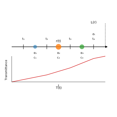
The pixel color C(r) for a ray r(t) = o + td with near and far bounds tn and tf is computed using the volume rendering integral:
where T(t) represents accumulated transmittance along the ray:
In practice, this continuous integral is approximated using numerical quadrature. For a set of sampled points along the ray {ti}Ni=1, the pixel color is estimated as:
where δi = ti+1 - ti is the distance between adjacent samples, and Ti is the accumulated transmittance up to sample i:
Hierarchical Sampling
To efficiently render scenes with complex view-dependent effects, NeRF employs a hierarchical sampling strategy. An initial "coarse" network predicts densities at uniformly spaced locations along each ray. These densities are then used to compute a piecewise-constant probability density function that guides sampling in a "fine" network, concentrating samples in regions likely to contribute significantly to the rendered color.
The probability wi that the i-th interval contains visible content is given by:
These weights are normalized to form a probability distribution for importance sampling in the fine network. This two-stage approach significantly improves rendering quality while maintaining computational efficiency.
Differentiable Rendering
A key innovation in NeRF is the use of differentiable volume rendering, which enables end-to-end training of the neural network from 2D images. The rendering process is formulated as a continuous function that can be differentiated with respect to the network parameters, allowing gradient-based optimization to learn the volumetric scene representation from multi-view images with known camera poses.

1.2 Traditional Methods vs. Neural Approaches
Traditional Volumetric Rendering Techniques
Traditional volumetric rendering methods rely on explicit geometric representations and physically-based light transport models. The most common approaches include:
- Ray Marching: Samples the volume along viewing rays, accumulating color and opacity using the volume rendering equation:
where \( T(t) = \exp\left(-\int_{t_n}^t \sigma(\mathbf{r}(s)) ds \right) \) is the transmittance, \( \sigma \) is the density, and \( \mathbf{c} \) is the radiance.
- Photon Mapping: Tracks photon paths through the volume to simulate complex light interactions
- Voxel Grids: Discretizes space into uniform 3D grids with precomputed optical properties
These methods require explicit scene geometry, careful parameter tuning, and significant computational resources for high-quality results.
Neural Radiance Fields (NeRF)
NeRF represents scenes implicitly using a continuous 5D function approximated by a multilayer perceptron (MLP):
where \( \mathbf{x} \in \mathbb{R}^3 \) is a 3D location, \( \mathbf{d} \in \mathbb{S}^2 \) is a viewing direction, \( \mathbf{c} \) is RGB color, and \( \sigma \) is volume density.
Key Advantages Over Traditional Methods:
- Continuous Representation: Avoids discretization artifacts of voxel grids
- View-Dependent Effects: Naturally models complex reflectance and transparency
- Memory Efficiency: Compresses scenes into network weights rather than explicit 3D data
Comparative Analysis
The table below highlights fundamental differences between the approaches:
| Feature | Traditional Methods | NeRF |
|---|---|---|
| Scene Representation | Explicit (meshes, voxels) | Implicit (neural network) |
| View Dependence | Separate BRDF models required | Learned end-to-end |
| Memory Scaling | O(n³) for voxel grids | O(1) with network size |
| Training Data | Geometry + material maps | Multi-view images only |
Performance Considerations
While traditional methods achieve real-time rendering through GPU acceleration of rasterization pipelines, NeRF's computational cost comes from:
Recent advances like Instant NGP use hash grids and smaller networks to achieve interactive rates, bridging the performance gap while maintaining NeRF's quality advantages.

1.3 Mathematical Formulation of Volume Rendering
Volume rendering computes the accumulated radiance along a ray passing through a participating medium. The fundamental equation governing this process is derived from radiative transfer theory, which models how light interacts with scattering and absorbing media. The core quantity is the transmittance $$T(t)$$, representing the probability that light travels from point $$t_0$$ to $$t$$ without being absorbed or scattered.
Deriving the Volume Rendering Equation
Consider a ray $$\mathbf{r}(t) = \mathbf{o} + t\mathbf{d}$$ with origin $$\mathbf{o}$$ and direction $$\mathbf{d}$$. The differential transmittance is governed by the extinction coefficient $$\sigma_t(\mathbf{r}(t))$$:
Solving this ordinary differential equation yields the transmittance between $$t_n$$ and $$t_f$$:
The volume rendering equation integrates emitted radiance $$L_e$$ and scattered light $$L_s$$ weighted by transmittance:
Numerical Integration via Quadrature
In practice, the integral is approximated using numerical quadrature. For a ray partitioned into $$N$$ segments with endpoints $$\{t_i\}_{i=1}^N$$, the discretized form becomes:
where:
- $$\alpha_i = 1 - \exp(-\sigma_i \delta_i)$$ is the opacity of segment $$i$$,
- $$\delta_i = t_{i+1} - t_i$$ is the segment length,
- $$T_i = \prod_{j=1}^{i-1} (1 - \alpha_j)$$ is the accumulated transmittance,
- $$c_i$$ is the emitted or scattered radiance.
Connection to NeRF
Neural Radiance Fields (NeRF) parameterize $$\sigma_t$$ and $$c_i$$ via a neural network. The network outputs density $$\sigma$$ and RGB color $$\mathbf{c}$$ at each 3D point, enabling differentiable volume rendering through:
This formulation allows end-to-end training by comparing rendered pixel colors with ground truth images using photometric loss.
2. Key Innovations of NeRF
Key Innovations of NeRF
Neural Radiance Fields as a Continuous Scene Representation
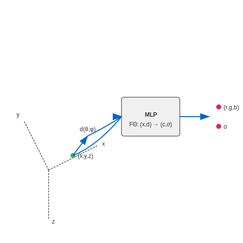
NeRF introduces a continuous volumetric scene function that maps a 3D spatial location (x, y, z) and viewing direction (θ, φ) to an emitted radiance c = (r, g, b) and volume density σ. This is represented as:
where F_Θ is a multilayer perceptron (MLP) with weights Θ. Unlike discrete voxel grids or point clouds, this formulation enables infinitely high-resolution reconstruction and view synthesis without memory constraints.
Differentiable Volume Rendering
NeRF employs a physically-based differentiable rendering equation to composite sampled 3D points along camera rays. The expected color C(r) for ray r(t) = o + td is computed via numerical quadrature:
where T(t) represents accumulated transmittance:
This formulation enables end-to-end training through backpropagation, as all operations (including the rendering integral) are differentiable.
Positional Encoding for High-Frequency Details
To overcome MLPs' bias toward low-frequency functions, NeRF applies a high-dimensional positional encoding to input coordinates before feeding them to the network:
For 3D coordinates, L=10 is typically used, expanding each scalar input to 60 dimensions. This allows the MLP to represent high-frequency scene details like texture and geometry discontinuities that would otherwise be smoothed out.
Hierarchical Volume Sampling
NeRF employs a two-stage importance sampling strategy to efficiently render scenes:
- A coarse network first samples 64 points per ray uniformly in depth
- A fine network then samples 128 additional points from the coarse network's probability distribution
This hierarchical approach concentrates samples in semantically relevant regions (e.g., near surfaces) while maintaining differentiability. The final rendered color combines outputs from both networks.
View-Dependent Appearance Modeling
By conditioning the radiance output c on viewing direction d, NeRF captures complex view-dependent effects like specular highlights and reflections. The network architecture splits computation:
- Density σ depends only on position x
- Color c depends on both x and d
This separation enforces physical constraints while allowing realistic material modeling. The viewing direction is typically encoded with L=4 frequency bands.
Architecture of a NeRF Model
The Neural Radiance Field (NeRF) model is a fully-connected deep neural network that maps 3D spatial coordinates $$ \mathbf{x} = (x, y, z) $$ and viewing directions $$ \mathbf{d} = ( heta, \phi) $$ to volume density $$ \sigma $$ and emitted radiance $$ \mathbf{c} = (r, g, b) $$. The architecture consists of two key components:
Core MLP Network
The backbone is an 8-layer multilayer perceptron (MLP) with ReLU activations that processes the 3D coordinates $$ \mathbf{x} $$. The first 5 layers output both a feature vector and the volume density $$ \sigma $$:
where $$ \mathbf{h} $$ is a 256-dimensional feature vector. The density $$ \sigma $$ is constrained to be positive using a softplus activation:
View-Dependent Radiance Prediction
The viewing direction $$ \mathbf{d} $$ is incorporated via an additional 3-layer MLP that predicts the RGB color $$ \mathbf{c} $$ from the feature vector $$ \mathbf{h} $$ and direction $$ \mathbf{d} $$:
where $$ \gamma(\cdot) $$ is a positional encoding function that projects low-dimensional inputs into a higher-dimensional space to better capture high-frequency details:
Hierarchical Sampling
NeRF employs a two-stage hierarchical sampling strategy to efficiently render rays:
- Coarse network: Samples 64 points per ray using stratified sampling to estimate the radiance field
- Fine network: Samples an additional 128 points per ray using importance sampling based on the coarse network's density estimates
The final rendered color $$ \hat{C}(\mathbf{r}) $$ for a ray $$ \mathbf{r}(t) = \mathbf{o} + t\mathbf{d} $$ is computed via numerical quadrature:
where $$ T_i = \exp\left(-\sum_{j=1}^{i-1} \sigma_j \delta_j\right) $$ is the accumulated transmittance and $$ \delta_i $$ is the distance between adjacent samples.
Positional Encoding
The model uses high-frequency positional encoding for both spatial coordinates and viewing directions to capture fine details. For coordinates, NeRF typically uses $$ L=10 $$ frequency bands (resulting in a 60-dimensional vector), while directions use $$ L=4 $$ bands (24-dimensional vector).
Implementation Details
- Network width: 256 neurons per layer
- Activation: ReLU for hidden layers, sigmoid for RGB output
- Positional encoding frequencies: $$ L=10 $$ for coordinates, $$ L=4 $$ for directions
- Batch size: 4096 rays per batch
- Optimizer: Adam with learning rate decay from 5e-4 to 5e-5

Training Data Requirements and Preparation
The quality and structure of training data significantly influence the performance of a Neural Radiance Field (NeRF) model. Unlike traditional supervised learning tasks, NeRF requires a carefully curated set of multi-view images with precise camera parameters to reconstruct a 3D scene accurately.
Image Capture Requirements
NeRF relies on a dense set of images covering the scene from multiple viewpoints. The following criteria must be met for optimal training:
- High Resolution: Images should be at least 1MP (megapixel) to capture fine details. Higher resolutions (4K+) improve reconstruction fidelity.
- Consistent Lighting: Avoid dynamic lighting conditions, as NeRF assumes static illumination per scene.
- Overlap and Coverage: Adjacent images should have at least 60-70% overlap to ensure robust view interpolation.
- Minimal Occlusions: Moving objects or obstructions during capture introduce artifacts in the reconstructed volume.
Camera Pose Estimation
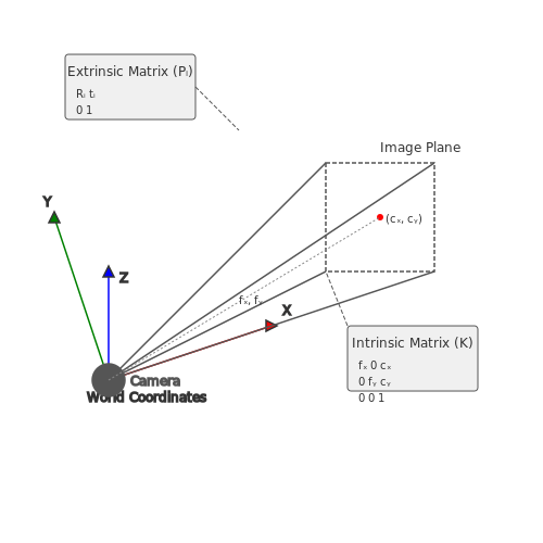
NeRF requires known camera intrinsics (focal length, principal point) and extrinsics (rotation, translation) for each image. These can be obtained via:
- Structure-from-Motion (SfM): Tools like COLMAP estimate camera poses from unordered images by matching feature points.
- Controlled Capture Rigs: Turntables or drone paths with known trajectories provide ground-truth poses.
- Depth Sensors: RGB-D cameras (e.g., Kinect) supply depth maps to refine pose estimation.
where K is the intrinsic matrix, and Pi represents the extrinsic matrix for the i-th image.
Data Preprocessing
Raw images often require preprocessing to align with NeRF's assumptions:
- White Balancing: Ensures color consistency across all views.
- Lens Distortion Correction: Radial and tangential distortions must be removed using calibrated camera parameters.
- Background Removal: For object-centric scenes, masking the background reduces noise in the reconstructed volume.
- Exposure Normalization: Linearizes pixel values if images have varying exposures.
Training Data Augmentation
While NeRF is data-hungry, synthetic augmentation must be applied carefully:
- View Synthesis: Novel views can be rendered via SfM-based interpolation, but overuse may cause blurring.
- Color Jitter: Minor adjustments in HSV space improve robustness to lighting variations.
- Patch Sampling: Training on random crops speeds up convergence but may lose global coherence.
Dataset Splitting
A standard split for NeRF training includes:
- Training (80%): Dense coverage of the scene for volume reconstruction.
- Validation (10%): Held-out views to tune hyperparameters like learning rate.
- Test (10%): Unseen viewpoints to evaluate generalization, measured via PSNR or SSIM.
For dynamic scenes, temporal consistency must be preserved in the split to avoid data leakage.
3. Setting Up the NeRF Pipeline
Setting Up the NeRF Pipeline
Coordinate System and Ray Sampling
The NeRF pipeline begins by defining a 3D coordinate system where scenes are represented implicitly. For each pixel in the input image, a camera ray r(t) = o + td is cast, where o is the ray origin (camera center), d is the normalized viewing direction, and t parameterizes the ray. To sample points along the ray, a stratified sampling approach divides the ray into N intervals, with points sampled uniformly within each interval.
This ensures dense sampling near surfaces while maintaining efficiency. Hierarchical sampling further optimizes this by focusing on regions with high density, as predicted by the coarse network.
Neural Network Architecture
The core of NeRF is a multilayer perceptron (MLP) that maps 3D coordinates x = (x, y, z) and viewing directions d = (θ, φ) to volume density σ and RGB color c. The network consists of two parts:
- A density network (8 fully connected layers with ReLU, 256 channels) that outputs σ and a feature vector.
- A view-dependent color network (1 fully connected layer, 128 channels) that conditions on the feature vector and viewing direction to predict c.
Positional encoding is applied to inputs to handle high-frequency details:
where L = 10 for coordinates and L = 4 for directions.
Volume Rendering Integral
The rendered color Ĉ(r) of a ray is computed via numerical integration using quadrature:
where T_i = exp(-\sum_{j=1}^{i-1} \sigma_j \delta_j) is the transmittance, and δ_i = t_{i+1} - t_i is the distance between samples. This differentiable rendering step enables end-to-end training.
Implementation Pipeline
The full pipeline involves these key steps:
- Data preparation: Load multi-view images with known camera poses (e.g., from COLMAP).
- Ray generation: For each training image, generate rays through all pixels.
- Hierarchical sampling: First pass with coarse sampling, then importance sampling.
- Network inference: Query the MLP at sampled 3D points.
- Volume rendering: Accumulate colors and densities using the rendering equation.
- Loss computation: Minimize the L2 loss between rendered and ground truth pixels.
# PyTorch pseudocode for NeRF rendering
def render_rays(rays, network_fn, N_samples):
    # Sample points along rays
    t_vals = torch.linspace(0., 1., N_samples)
    pts = rays.o[...,None,:] + rays.d[...,None,:] * t_vals[...,None]

    # Query network
    raw = network_fn(pts)
    rgb = torch.sigmoid(raw[...,:3])
    sigma = F.relu(raw[...,3])

    # Compute weights
    dists = t_vals[...,1:] - t_vals[...,:-1]
    alpha = 1. - torch.exp(-sigma * dists)
    weights = alpha * torch.cumprod(1.-alpha + 1e-10, -1)

    # Composite
    rgb_map = torch.sum(weights[...,None] * rgb, -2)
    return rgb_map
Optimization Details
Training uses the Adam optimizer with a learning rate of 5×10⁻⁴, decaying exponentially to 5×10⁻⁵. A batch size of 1024 rays is typical, with equal sampling from all images to prevent bias. The two-stage hierarchical sampling uses Nc = 64 coarse and Nf = 128 fine samples per ray.

3.2 Sampling Strategies for Efficient Training
NeRF's volumetric rendering requires densely sampling points along camera rays to compute the integral of radiance and opacity. Naive uniform sampling is computationally expensive and inefficient, as most samples contribute negligibly to the final rendered color. Advanced sampling strategies focus computation on regions with high opacity or radiance variation, dramatically improving training efficiency.
Hierarchical Sampling
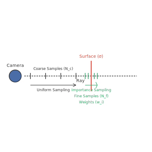
The original NeRF paper proposes a two-stage hierarchical sampling approach. First, a coarse network evaluates Nc uniformly distributed samples along each ray to estimate an initial density distribution. This coarse distribution informs the allocation of Nf fine samples, concentrating them in regions likely to contain surfaces.
where wi are the weights from the coarse network, Ti is accumulated transmittance, σi is density, and δi is the distance between samples. These weights define a piecewise-constant PDF used for importance sampling in the fine stage.
Inverse Transform Sampling
Given the piecewise-constant PDF from coarse weights, fine samples are drawn using inverse transform sampling:
where F is the CDF constructed from the normalized weights. This ensures samples are drawn proportional to their expected contribution to the rendered color.
Stratified Sampling
To prevent clustering of samples and maintain good coverage, the sampling intervals are divided into Nf bins, with one sample drawn uniformly from each bin before applying the inverse transform. This stratified approach reduces variance compared to pure importance sampling.
Learned Sampling with Proposal Networks
Recent advances like Mip-NeRF and Instant NGP replace the coarse network with learned proposal networks that predict sampling distributions more efficiently. These networks output a series of piecewise-constant density distributions that are progressively refined:
where the proposal MLP predicts densities without view dependence, enabling faster evaluation. Multiple proposal stages (typically 2-3) allow coarse-to-fine optimization of the sampling distribution.
Occupancy Grid Acceleration
Methods like Instant NGP combine learned sampling with multi-resolution hash grids to skip empty space. An occupancy grid tracks which regions contain significant density, allowing the renderer to skip samples in known-empty regions entirely. The grid is updated during training based on observed densities.
# Pseudocode for occupancy grid sampling
def sample_along_ray(ray_origin, ray_direction, occupancy_grid):
    samples = []
    t = near
    while t < far:
        if occupancy_grid.query(ray_origin + t*ray_direction):
            samples.append(t)
            t += base_step
        else:
            t += empty_skip_step
    return samples
Adaptive Sampling with Uncertainty
Some approaches use predictive variance to guide sampling. By training an auxiliary network to estimate uncertainty in the radiance field, samples can be concentrated in regions where the model is uncertain:
where Ĉ(r) is the predicted color variance. This is particularly effective for capturing fine details and sharp discontinuities.
3.3 Optimizing Rendering Quality and Speed
NeRF's volumetric rendering pipeline achieves photorealistic novel view synthesis but suffers from high computational demands. The rendering integral for a pixel's color C along ray r with near/far bounds tn, tf is:
where T(t) = exp(-∫tntσ(r(s))ds) models accumulated transmittance. Practical implementations approximate this via quadrature with N samples:
Hierarchical Sampling Strategies
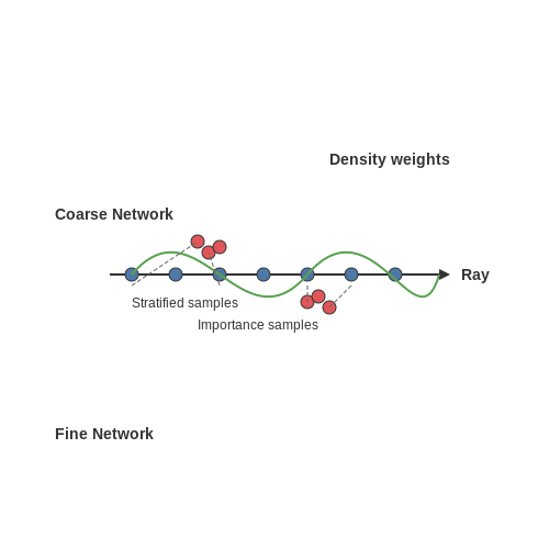
Uniform sampling wastes computation on empty or occluded regions. Two-stage hierarchical sampling improves efficiency:
- Coarse network: Evaluates at Nc stratified samples to estimate density distribution
- Fine network: Allocates Nf samples proportionally to coarse weights
The combined probability density function becomes:
Positional Encoding Tradeoffs
NeRF's high-frequency positional encoding γ(p) = (sin(20πp), cos(20πp), ..., sin(2L-1πp), cos(2L-1πp)) enables sharp details but requires careful frequency selection:
- Lower L values (5-6 for position, 3-4 for direction) prevent aliasing artifacts
- Progressive encoding during training stabilizes optimization
Network Architecture Optimizations
Recent variants improve the MLP backbone:
| Method | Parameters | Speedup |
|---|---|---|
| Original NeRF | 1.3M | 1× |
| Instant NGP | 15K | 1000× |
| Plenoxels | 75M | 100× |
Ray Marching Acceleration
Empty space skipping via occupancy grids or octrees reduces sampled regions. The conditional sampling probability becomes:
where O is a binary occupancy indicator. Modern implementations achieve real-time rendering by combining:
- 16-bit half-precision inference
- Tensor cores for fused MLP evaluation
- Speculative execution of ray batches
4. Dynamic Scene Modeling with NeRF
Dynamic Scene Modeling with NeRF
Extending NeRF to model dynamic scenes introduces significant challenges, as the original formulation assumes static geometry and lighting. The core problem lies in disentangling temporal variations in geometry, appearance, and viewpoint while maintaining photorealistic rendering quality. Recent approaches address this through either explicit deformation fields or implicit time-conditioned representations.
Deformation Field Approaches
Methods like D-NeRF introduce a deformation field D(x, t) that maps points from canonical space to their time-dependent positions:
where x is the canonical 3D coordinate and t is the time parameter. The field is typically implemented as an MLP that takes positional encoding of both spatial coordinates and time:
This approach requires careful regularization to prevent degenerate solutions where the deformation field collapses all points to a single location. A common solution is to add a rigidity loss that penalizes non-isometric transformations:
where J is the Jacobian of the deformation field and I is the identity matrix.
Time-Conditioned Radiance Fields
Alternative approaches like NSFF and HyperNeRF treat time as an additional input dimension to the radiance field MLP:
This formulation allows modeling of complex non-rigid deformations but requires significantly more training data to avoid overfitting. The temporal dimension introduces a 4D reconstruction problem where the inherent ambiguity between view-dependent effects and actual scene motion must be carefully resolved.
Motion Decomposition Techniques
State-of-the-art methods employ hierarchical representations to separate different motion components:
- Rigid body motion: Modeled through SE(3) transformations
- Non-rigid deformation: Represented as residual displacements
- Topological changes: Handled via learned attention mechanisms
The rendering equation for dynamic scenes extends the volume rendering integral to include temporal dependence:
where the accumulated transmittance T(t) now depends on both spatial and temporal coordinates.
Implementation Challenges
Training dynamic NeRFs presents several practical considerations:
- Temporal sampling must be dense enough to avoid motion aliasing
- Memory requirements grow linearly with the number of timesteps
- Optical flow constraints are often needed to regularize motion fields
- Background/foreground separation becomes critical for unconstrained scenes
Recent work has shown that incorporating physical priors (e.g., fluid dynamics equations for liquid simulations) can significantly improve generalization when training data is limited. The field continues to evolve with hybrid approaches that combine explicit surface representations with neural radiance fields for improved temporal coherence.

4.2 Handling Sparse Input Views
The Sparse View Challenge in NeRF
NeRF’s performance degrades significantly when trained on sparse input views (fewer than 10 images) due to the underconstrained nature of the inverse rendering problem. The radiance field σ(x) and RGB emission c(x, d) become ambiguous when observed from limited angles, leading to:
- Geometry artifacts: Floating surfaces or holes due to insufficient multi-view consistency
- View-dependent effects: Incorrect specular highlights that violate physical light transport
- Background collapse: Unobserved regions defaulting to empty space or noisy densities
Regularization Techniques
Current approaches introduce explicit inductive biases through loss terms:
Where ℒdepth uses sparse depth supervision from COLMAP or LiDAR:
And ℒnormal enforces surface smoothness through predicted normals:
Latent Space Completion Methods
Recent work (e.g., PixelNeRF, RegNeRF) employs:
- Feature diffusion: CNN-based encoders propagate features to unobserved regions
- GAN-based inpainting: Adversarial training fills in missing geometry
- Transformer attention: Cross-view feature aggregation via attention mechanisms
Hybrid Explicit-Implicit Representations
Methods like DS-NeRF combine:
- Sparse voxel grids for coarse geometry
- Hash tables for efficient empty space skipping
- MLPs for view-dependent effects
The hybrid approach reduces the solution space by constraining the MLP to plausible configurations given the explicit prior.
Real-Time Rendering Approximations
Traditional NeRF rendering relies on computationally expensive ray marching and volume integration, making real-time performance challenging. To address this, several approximation techniques have been developed that trade off some accuracy for significant speed improvements.
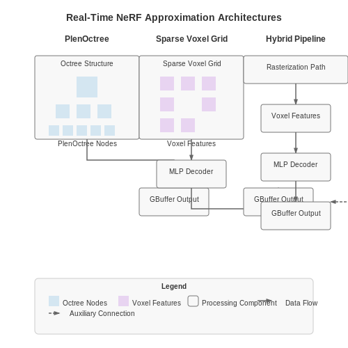
PlenOctrees and Sparse Voxel Grids
One approach replaces the continuous neural radiance field with a discrete hierarchical data structure. The PlenOctree method precomputes and stores spherical harmonic coefficients in an octree, enabling fast lookup during rendering. The rendering equation simplifies to:
where $$T_i$$ is the transmittance, $$\alpha_i$$ the opacity, and $$c_i$$ the precomputed radiance at voxel $$i$$. This reduces the rendering complexity from O(N) neural network evaluations to O(log N) tree traversals.
Neural Sparse Voxel Fields
An extension combines sparse voxel grids with small MLPs at each voxel. The grid stores features that are decoded by compact networks, maintaining some neural capacity while enabling:
- Frustum culling of invisible regions
- Level-of-detail rendering
- Hardware-accelerated ray tracing
Hybrid Neural Rasterization
Some methods combine neural rendering with traditional rasterization pipelines. The neural network predicts:
where the G-buffer contains material properties that are then shaded using conventional real-time techniques. This approach leverages existing GPU rasterization hardware while maintaining view-dependent effects.
Importance Sampling Strategies
For cases where neural evaluation is unavoidable, importance sampling methods significantly reduce the number of required samples:
Practical implementations use:
- Proposal networks that predict sampling distributions
- Reservoir sampling for temporal reuse
- Adaptive sampling based on expected contribution
Hardware-Specific Optimizations
Modern implementations exploit GPU hardware features:
- Tensor cores for mixed-precision MLP evaluation
- Ray tracing cores for accelerated intersection tests
- Shader programming tricks for memory coalescing
The tradeoffs between these approaches can be characterized by their error metrics and frame rates:
| Method | PSNR (dB) | FPS |
|---|---|---|
| Original NeRF | 32.5 | 0.1 |
| PlenOctree | 30.8 | 60 |
| Sparse Voxel | 31.2 | 30 |
| Hybrid | 29.7 | 120 |
5. NeRF in Virtual and Augmented Reality
5.1 NeRF in Virtual and Augmented Reality
Challenges in Real-Time Volumetric Rendering
The primary bottleneck in deploying Neural Radiance Fields (NeRF) in virtual and augmented reality (VR/AR) is computational latency. Traditional NeRF architectures require hundreds of network evaluations per pixel to render a single frame, making real-time performance infeasible for interactive applications. The volumetric rendering integral for a ray r(t) is given by:
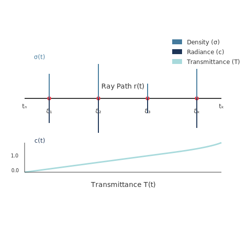
where T(t) is the transmittance, σ the volume density, and c the radiance. Real-time implementations must approximate this integral with fewer samples while preserving visual fidelity.
Optimization Techniques for VR/AR
Recent advances address this through hybrid representations and neural caching:
- Plenoxels combine sparse voxel grids with spherical harmonics for faster density queries
- Instant NGP uses multiresolution hash tables to reduce MLP inference cost
- KiloNeRF decomposes the scene into thousands of small MLPs for parallel evaluation
The rendering equation can be reformulated for real-time applications using importance sampling based on a coarse geometry proxy:
Latency and Bandwidth Considerations
For AR applications on mobile devices, the memory footprint of neural representations becomes critical. A compressed NeRF model typically requires:
where n denotes MLP widths, s the grid resolution at level l, and b the bits per voxel. State-of-the-art methods achieve 50-100MB models for room-scale environments with 2-5ms rendering times on mobile GPUs.
Tracking and Dynamic Scenes
Incorporating NeRF into VR systems requires solving the simultaneous localization and mapping (SLAM) problem. The camera pose estimation can be formulated as:
where ξ represents the 6DOF camera pose and π the projection function. Recent work combines differentiable rendering with inertial measurement unit (IMU) data for robust tracking.
Case Study: Varjo XR-4 Implementation
The Varjo XR-4 headset demonstrates a production NeRF pipeline achieving:
- 90Hz refresh rate at 2880×2720 per-eye resolution
- 2.3ms end-to-end latency using foveated rendering
- Sub-millimeter positional tracking accuracy
This is enabled by a custom neural acceleration structure that caches radiance fields in a sparse octree representation, with dynamic updates limited to view-dependent effects in the foveal region.
Medical Imaging and Scientific Visualization
Neural Radiance Fields (NeRF) have demonstrated remarkable potential in medical imaging and scientific visualization by enabling high-fidelity volumetric reconstructions from sparse 2D inputs. Unlike traditional methods such as computed tomography (CT) or magnetic resonance imaging (MRI), which rely on explicit voxel grids, NeRF implicitly represents volumetric data as a continuous function, allowing for higher resolution and more efficient memory usage.
NeRF for Medical Volumetric Reconstruction
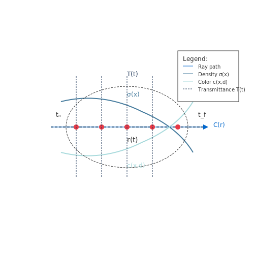
In medical applications, NeRF can reconstruct 3D anatomical structures from a limited set of 2D X-ray, ultrasound, or endoscopic images. The key advantage lies in its ability to model complex tissue densities and light interactions without requiring dense sampling. The radiance field σ(x) represents the density at point x, while c(x, d) encodes the view-dependent color. The volume rendering integral computes the expected color C(r) for a ray r(t) as:
where T(t) is the accumulated transmittance along the ray:
This formulation enables precise modeling of semi-transparent tissues, such as vasculature or neural fibers, which are challenging for traditional mesh-based representations.
Adaptations for Scientific Data
Scientific visualization often deals with scalar or vector fields, such as fluid dynamics simulations or molecular structures. NeRF can be extended to represent these fields by modifying the output of the neural network to include additional physical quantities. For example, in computational fluid dynamics (CFD), the network can predict velocity v(x) and pressure p(x) alongside density and color:
This allows for interactive exploration of complex phenomena like turbulence or shock waves without resorting to grid-based interpolation.
Case Study: NeRF in MRI Super-Resolution
A recent breakthrough involves using NeRF to enhance low-resolution MRI scans. By training on paired low- and high-resolution scans, the network learns to predict high-frequency details missing in the input. The loss function incorporates perceptual metrics to ensure anatomical accuracy:
where LPIPS (Learned Perceptual Image Patch Similarity) ensures structural consistency with ground truth data.
Challenges and Future Directions
Despite its promise, NeRF faces challenges in medical applications. Training requires careful handling of noise and artifacts in clinical images, and real-time inference remains computationally intensive. Hybrid approaches, combining NeRF with traditional segmentation networks, are being explored to balance accuracy and speed. Future work may focus on integrating physics-based constraints, such as biomechanical properties, to further improve realism and diagnostic utility.
5.3 Challenges in Real-World Deployment
Computational Complexity and Rendering Speed
NeRF's volumetric rendering requires evaluating millions of 3D points along rays for each pixel, leading to high computational demands. The rendering process involves querying a neural network at each sampled point, which scales with resolution as:
where Nrays scales quadratically with image resolution, Nsamples is typically 64-256 samples per ray, and Dnetwork is the depth of the MLP. Even with optimizations like hierarchical sampling, real-time rendering at HD resolutions remains challenging without specialized hardware.
Generalization Across Scenes
Standard NeRF models are scene-specific - each new environment requires full retraining from scratch. This limitation stems from:
- No shared geometric priors: The MLP learns only local scene properties without cross-scene transfer
- View consistency requirements: Training images must cover the scene comprehensively (typically 50-100 images)
- Lighting sensitivity: Models often bake in illumination conditions present during training
Recent work in generalizable NeRFs attempts to address this through meta-learning or transformer architectures, but these approaches still lag behind single-scene quality.
Dynamic Scene Modeling
The original NeRF formulation assumes static scenes. Modeling dynamics requires either:
where time t becomes an additional input dimension. This expansion introduces several challenges:
- Temporal coherence: Avoiding flickering artifacts requires careful regularization
- Memory growth: 4D representations demand significantly more capacity
- Training data: Requires synchronized multi-view video instead of still images
Material and Lighting Decomposition
NeRF's radiance field c(x,d) conflates material properties with lighting effects. This causes several practical issues:
- Relighting difficulty: Changing illumination requires expensive retraining
- Editability limitations: Modifying specific objects or materials is non-trivial
- Physical inaccuracy: The learned BRDF may not obey energy conservation
Recent extensions like NeRF-W and PhySG attempt to separate illumination from reflectance through additional network branches or physical constraints.
Robustness to Imperfect Inputs
Real-world capture conditions often violate NeRF's ideal assumptions:
- Imperfect camera calibration: Pose errors degrade reconstruction quality
- Partial occlusions: Missing viewpoints create "floaters" in the volume
- Transient objects: Moving elements during capture cause artifacts
Current solutions involve:
where auxiliary losses from depth sensors or optical flow help constrain the optimization.
6. Key Research Papers on NeRF
6.1 Key Research Papers on NeRF
- PDF Scientific Visualization, 2025, volume 17, number 1, pages 65 - 85, DOI ... — Scientific Visualization, 2025, volume 17, number 1, pages 65 - 85, DOI: 10.26583/sv.17.1.06 Application of PyTorch3D and NERF Computer Vision Tools for Building a Point Cloud of a Three-Dimensional Model and Determining the Camera Position of Still Images in Space V.V. Konkov1, A.B. Zamchalov2
- SpNeRF: Memory Efficient Sparse Volumetric Neural Rendering Accelerator ... — SpNeRF: Memory Efficient Sparse Volumetric Neural Rendering Accelerator for Edge Devices Yipu Zhang 1, Jiawei Liang , Jian Peng , Jiang Xu2, Wei Zhang1,∗ 1Department of Electronic and Computer Engineering, The Hong Kong University of Science and Technology 2Microelectronics Thrust, The Hong Kong University of Science and Technology (GZ) {yzhangqg, jliangbr, jpengai}@connect.ust.hk, jiang.xu ...
- Drone-NeRF: Efficient NeRF based 3D scene ... - ScienceDirect — 3) Volumetric rendering yields confined RGB and Depth attributes while simultaneously addressing shadows originating from vertical planes based on overlap and compensation areas. The expansion of sub-scene boundaries compensates for occluded regions, resulting in a seamless and refined scene representation through the coherent stages of the ...
- L2H-NeRF: low- to high-frequency-guided NeRF for 3D ... - Springer — In this paper, we propose an innovative low- to high-frequency-guided NeRF (L2H-NeRF) framework that decomposes scene reconstruction into coarse and fine stages. For the first stage, a low-frequency enhancement network based on a vision transformer is proposed, where the low-frequency-based globally coherent geometric structure is recovered ...
- Neural Radiance Fields with Hash-Low-Rank Decomposition - MDPI — In recent advancements in novel view synthesis and neural rendering, neural radiance field (NeRF) has emerged as a powerful technique for synthesizing high-quality novel views of complex 3D scenes. However, the computational and storage demands of NeRF limit its applicability. In this paper, we present a novel approach to NeRF by combining low-rank decomposition and multi-hash encoding through ...
- NeRF: Representing Scenes as Neural Radiance Fields for View Synthesis — An overview of our neural radiance field scene representation and differentiable rendering procedure. We synthesize images by sampling 5D coordinates (location and viewing direction) along camera rays (a), feeding those locations into an MLP to produce a color and volume density (b), and using volume rendering techniques to composite these values into an image (c).
- D-NeRF: Neural Radiance Fields for Dynamic Scenes - ResearchGate — Neural radiance fields (NeRF) encode a scene into a neural representation that enables photo-realistic rendering of novel views. However, a successful reconstruction from RGB images requires a ...
- NeRF - Communications of the ACM — To render this neural radiance field (NeRF) from a particular viewpoint, we: 1) march camera rays through the scene to generate a sampled set of 3D points, 2) use those points and their corresponding 2D viewing directions as input to the neural network to produce an output set of colors and densities, and 3) use classical volume rendering ...
- FoV-NeRF: Foveated Neural Radiance Fields for Virtual Reality — We find that our method significantly reduces latency (up to 99% time reduction compared with NeRF) without loss of high-fidelity rendering (perceptually identical to full-resolution ground truth).
- High Dynamic Range Novel View Synthesis with Single Exposure - ResearchGate — High Dynamic Range Novel View Synthesis (HDR-NVS) aims to establish a 3D scene HDR model from Low Dynamic Range (LDR) imagery. Typically, multiple-exposure LDR images are employed to capture a ...
6.2 Open-Source Implementations and Tools
- Magic NeRF lens: interactive fusion of neural radiance fields for ... — 3.2.2 Magic NeRF lens with FoV restrictor. While designs described in Section 3.2.1 enable dynamic manipulation and editing of NeRF models, several considerations from DG1 and DG2 are not met. For example, when inspecting facility equipment that covers a substantial area of volume, the increased latency in VR NeRF rendering on devices with limited computational resources will lead to the ...
- Volumetric Rendering with Baked Quadrature Fields - arXiv.org — Figure 1: We propose using textured polygons with NeRF to efficiently render non-opaque scenes, combining high-quality rendering with modern graphics hardware. To model a scene, we produce a mesh that gives quadrature points along a ray (shown as points on the intersection with the cross-section of the mesh) required in volumetric rendering.
- Magic NeRF lens: interactive fusionofneuralradiance fieldsfor - Frontiers — complementary strengths of volumetric rendering and geometric rasterization. As Figure 1A illustrates, the photorealistic rendering of a NeRF model is merged with the polygonal representation of its corresponding CAD models, creating a 3D-magic-lens-style visualization (Viega et al., 1996) and achieving render volume reduction without
- PDF FastSR-NeRF: Improving NeRF Efficiency on Consumer Devices with A ... — NeRF can be trained on consumer devices such as a Mac-Book Air M2, whereas most other models and existing NeRF+SR pipelines fail to train with a meaningful time budget. Overall, our analysis shows that SR can be a low-cost, plug-and-play strategy for improving the efficiency of neu-ral rendering models under a limited training budget. Even
- Don't Splat your Gaussians: Volumetric Ray-Traced Primitives for ... — In parallel, volume-rendering techniques and continuous volumetric representations have recently seen unprecedented interest in the fields of computer vision and image-based graphics, spearheaded by efforts such as neural radiance fields [Mildenhall et al. 2020].These methods allow us to capture and render photorealistic three-dimensional scenes by optimizing an underlying volumetric ...
- Neural radiance fields in the industrial and robotics domain ... — Images are synthesized from NeRF using traditional volumetric rendering, ... NeRFs that can generate the desired 3D model from scratch can partially supplement or even fulfill the role of CAD tools in the future. ... Its significant advantage is an existing open source implementation that facilitates the rapid and reproducible setup of dynamic ...
- TraM‐NeRF: Tracing Mirror and Near‐Perfect Specular Reflections Through ... — Combining NeRF volume rendering and ray-tracing with physically plausible materials at intersection points introduces an inductive bias into the training of TraM-NeRF that enables it to learn a single coherent scene representation, even when geometry has only been observed in a reflection. ... The source code of our implementation is available ...
- NeuVV: Neural Volumetric Videos with Immersive Rendering and Editing — We further develop a hybrid neural-rasterization rendering framework to support consumer-level VR headsets so that the aforementioned volumetric video viewing and editing, for the first time, can ...
- Real-Time Volume Graphics | PDF | Shader | Rendering (Computer ... - Scribd — Volume-Rendering Integral The emission-absorption optical model leads to the volumerendering integral: D s0 (t) dt. I(D) = I0 e + s0. q(s) e. D s (t) dt. ds , (1.7) with optical properties (absorption coecient) and q (source term describing emission) and integration from entry point into the volume, s = s0 , to the exit point toward the camera ...
- PDF Point-NeRF: Point-Based Neural Radiance Fields - CVF Open Access — Figure 1. Point-NeRF uses neural 3D points to efficiently represent and render a continuous radiance volume. The point-based radiance field can be predicted via network forward inference from multi-view images. It can then be optimized per scene to achieve reconstruction quality that surpasses NeRF [34] in tens of minutes.
6.3 Recommended Tutorials and Courses
- EVER: Exact Volumetric Ellipsoid Rendering for Real-time View Synthesis — The field of 3D reconstruction for novel view synthesis has explored a variety of scene representations: point based [22], surface based [26, 46, 43], and volume based [29, 31].Since their introduction in NeRF [29], differentiable rendering of volumetric scene representations have become popular due to their ability to yield photorealistic 3D reconstructions.
- GitHub - facebookresearch/pytorch3d: PyTorch3D is FAIR's library of ... — Get started with PyTorch3D by trying one of the tutorial notebooks. Deform a sphere mesh to dolphin: ... no guarantee. Best efforts to communicate breaking changes and facilitate migration of code or data (incl. models). ... PyTorch3D v0.4.0 released with support for implicit functions, volume rendering and a reimplementation of NeRF. [November ...
- NeRF: Representing Scenes as Neural Radiance Fields for View Synthesis — To render this neural radiance field (NeRF) from a particular viewpoint we: 1) march camera rays through the scene to generate a sampled set of 3D points, 2) use those points and their corresponding 2D viewing directions as input to the neural network to produce an output set of colors and densities, and 3) use classical volume rendering ...
- GitHub - kwea123/nerf_Unity: Unity project for nerf_pl (Neural Radiance ... — This project is built on Unity 2019.3.9f1 on Windows.It contains 3 scenes (under Scenes/ folder):. MeshRender; MixedReality; VolumeRender; Due to large size of the files, I put the assets in release, you need to download from there and import to Unity. Make sure you download them and put under Assets/ before opening Unity. Follow the instructions below for each scene:
- NeuVV: Neural Volumetric Videos with Immersive Rendering and Editing — We further develop a hybrid neural-rasterization rendering framework to support consumer-level VR headsets so that the aforementioned volumetric video viewing and editing, for the first time, can ...
- GitHub - bneal3/nerf-volrend: PlenOctree Volume Rendering (supports ... — If you do not have CUDA-capable GPU, pass -DVOLREND_USE_CUDA=OFF after cmake .. to use fragment shader backend, which is also used for the web demo. It is slower and does not support mesh-insertion and dependent features such as lumisphere probe. The main real-time PlenOctree rendererer volrend and a headless version volrend_headless are built. The latter requires CUDA.
- Volume Rendering Using Arnold | Free Tutorial Series - REBELWAY 2.0 — It's best to use the latest shader that ships with Arnold 6 by using the IPR and tweaking the value you should see so you have a clear indication of what the result looks like. The cloud chapter contains an updated hip file that is made using the latest Houdini and Arnold version. Volume Rendering Using Arnold Tutorial Series: What to Expect ...
- Volume visualization and volume rendering techniques - ResearchGate — This course will give an introduction to the volume rendering transport theory and the involved issues such as interpolation, illumination, classification and others. Different volume rendering ...
- PDF CS5670: Computer Vision - Department of Computer Science — Novak et al 2018, Monte Carlo methods for physically based volume rendering Porter and Duff 1984, Compositing Digital Images Physically-based Monte Carlo rendering [Novak et al]
- Monte Carlo methods for physically based volume rendering - Wojciech Jarosz — The goal of this course is to complement a recent Eurographics 2018 state-of-the-art report providing a broad overview of most techniques developed to date, including a few methods from neutron transport, with a focus on concepts that are most relevant to CG practitioners. ... Monte Carlo methods for physically based volume rendering. ACM ...