Fashion Compatibility Predictor Using AI
1. Defining Fashion Compatibility in AI Systems
Defining Fashion Compatibility in AI Systems
Fashion compatibility in AI systems refers to the computational modeling of aesthetic and functional harmony between clothing items, accessories, or outfits. Unlike traditional recommendation systems that rely on user preferences or item popularity, fashion compatibility predictors leverage deep learning to quantify stylistic coherence based on visual, textual, and contextual features. The problem is inherently multimodal, requiring joint embeddings of images, text descriptions, and metadata to capture latent relationships.
Mathematical Formulation
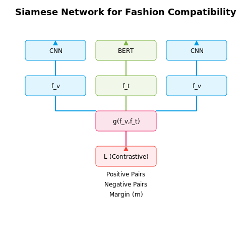
Given a set of fashion items X = {x1, x2, ..., xn}, where each item xi is represented by a feature vector fi ∈ ℝd, compatibility is modeled as a pairwise scoring function s: ℝd × ℝd → [0, 1]. The function s(fi, fj) predicts the likelihood that items xi and xj are stylistically compatible. A common approach uses a Siamese neural network with contrastive loss:
where 𝒫 denotes positive (compatible) pairs, 𝒩 denotes negative (incompatible) pairs, and m is a margin hyperparameter enforcing separation between incompatible items.
Feature Extraction
Modern systems employ convolutional neural networks (CNNs) for visual feature extraction and transformer-based models for textual metadata. For an image I, a CNN backbone (e.g., ResNet-50) produces a visual embedding fv = CNN(I). Textual descriptions T are encoded via BERT or similar models:
These embeddings are fused through attention mechanisms or late fusion to form a joint representation f = g(fv, ft), where g is a learnable function (e.g., MLP or cross-modal transformer).
Evaluation Metrics
Standard evaluation protocols include:
- Area Under the ROC Curve (AUC): Measures ranking performance of compatible vs. incompatible pairs.
- Top-k Accuracy: Proportion of test queries where a compatible item is retrieved in the top k recommendations.
- Fill-in-the-Blank (FITB): Given a partial outfit, the model selects the most compatible item from a candidate set.
Challenges and Edge Cases
Key challenges include:
- Subjectivity: Compatibility judgments vary across cultures, demographics, and personal tastes.
- Cold Start: Handling new items with limited interaction data.
- Context Sensitivity: An item may be compatible in casual settings but not formal ones.
State-of-the-art approaches address these by incorporating user-specific embeddings or leveraging graph neural networks to model outfit-level dependencies.
Key Challenges in Predicting Outfit Compatibility
Subjectivity in Fashion Aesthetics
Fashion compatibility prediction is inherently subjective, as aesthetic preferences vary across cultures, demographics, and personal tastes. Unlike objective tasks like object detection, where ground truth labels are unambiguous, outfit compatibility lacks a universally accepted metric. This subjectivity complicates the creation of labeled datasets, as human annotators often disagree on what constitutes a "compatible" outfit. The problem can be formalized as learning a compatibility function f: (i, j) → [0,1], where i and j are fashion items, and the output represents their compatibility score. However, the ground truth for this function is noisy and context-dependent.
Here, yk(i, j) represents the compatibility judgment of the kth annotator, and N is the total number of annotators. The variance in yk(i, j) highlights the challenge of obtaining reliable training data.
High-Dimensional Feature Space
Fashion items are characterized by multiple attributes, including color, texture, pattern, silhouette, and style. Representing these attributes in a machine learning model requires high-dimensional embeddings, which introduce computational and generalization challenges. For instance, a deep neural network might process an image through a convolutional backbone to extract a feature vector v ∈ ℝd, where d can range from 512 to 2048 dimensions. The compatibility function must then operate in this high-dimensional space, requiring careful regularization to avoid overfitting.
Contextual and Seasonal Dependencies
Outfit compatibility is context-sensitive. A winter coat paired with shorts may be incompatible in summer but acceptable in a transitional season. Similarly, formal and casual contexts impose different compatibility constraints. Modeling these dependencies requires temporal and contextual signals, often absent in static datasets. Recent approaches use attention mechanisms to weight compatibility scores based on contextual features:
where Wc is a weight matrix, vi and vj are item embeddings, c is a context vector, and σ is a sigmoid activation.
Data Sparsity and Long-Tail Distribution
Fashion datasets suffer from a long-tail distribution, where a few popular items dominate the dataset, while many others appear infrequently. This sparsity makes it difficult to learn reliable compatibility metrics for rare items. Metric learning approaches, such as triplet loss, struggle when negative samples are uninformative or when positive pairs are scarce. Techniques like negative sampling hard mining or synthetic data augmentation are often employed to mitigate this issue.
Multi-Modal Fusion
Effective compatibility prediction requires fusing information from multiple modalities—visual (images), textual (product descriptions), and categorical (brand, category tags). Each modality provides complementary signals, but aligning them into a unified representation is non-trivial. Cross-modal attention networks have shown promise, but they require large-scale training data and careful hyperparameter tuning to avoid modality dominance.
Real-World Deployment Challenges
In production systems, outfit compatibility models must handle real-time inference, scalability across millions of items, and user feedback integration. Latency constraints often necessitate approximate nearest-neighbor search in the embedding space, which can degrade performance. Additionally, user interactions (e.g., clicks, purchases) provide implicit feedback, but incorporating this data requires robust online learning mechanisms to avoid feedback loops.
1.3 Role of Visual and Contextual Features in Fashion AI
Fashion compatibility prediction relies on extracting and modeling two primary feature categories: visual features and contextual features. Visual features capture the aesthetic and stylistic properties of garments, while contextual features encode semantic relationships between items based on usage scenarios, seasons, or cultural norms.
Visual Feature Extraction
Convolutional Neural Networks (CNNs) form the backbone of visual feature extraction, with ResNet-50 and Vision Transformers (ViTs) achieving state-of-the-art performance. The feature vector fv for an image I is computed through a series of nonlinear transformations:
where φ represents the CNN/ViT encoder and θ denotes the learned parameters. Key visual attributes include:
- Color histograms in LAB space for perceptual accuracy
- Texture patterns via Gabor filter banks
- Shape descriptors using HOG (Histogram of Oriented Gradients)
- Local semantic features from attention maps in ViTs
Contextual Feature Representation
Contextual features fc capture relational dynamics between fashion items. These are modeled through:
where ψ is a graph neural network (GNN) operating on items gi with adjacency matrix W. Contextual dimensions include:
- Co-occurrence statistics from large-scale outfit datasets
- Temporal context (seasonality, trends) via LSTM temporal modeling
- Social context derived from user behavior graphs
- Semantic embeddings of product descriptions using BERT
Feature Fusion Architectures
Modern compatibility models employ cross-modal fusion strategies. Let fv(i) and fc(i) denote features for item i. The compatibility score sij between items i and j is computed through:
where ⊕ denotes concatenation and σ is the sigmoid function. Advanced approaches use:
- Cross-attention mechanisms to model feature interdependencies
- Metric learning with triplet losses in the joint embedding space
- Transformer-based fusion with learned query-key-value projections
Case Study: Polyvore Outfit Compatibility
The Polyvore dataset demonstrates the importance of feature combination. Using only visual features achieves 68.2% accuracy in outfit compatibility prediction, while incorporating contextual features (co-occurrence, descriptions) boosts performance to 82.7%. The state-of-the-art model (ACMR, CVPR 2021) combines:
- Visual features from a ViT-L/16 backbone
- Contextual graph embeddings with relational attention
- Multi-task learning on complementary and substitute relationships
This achieves 89.3% accuracy on the Polyvore-D test set, demonstrating the synergistic effect of visual-contextual feature fusion.

2. Sourcing and Curating Fashion Datasets
Sourcing and Curating Fashion Datasets
Publicly Available Fashion Datasets
Several high-quality fashion datasets are publicly accessible for research in compatibility prediction. The DeepFashion dataset contains over 800,000 diverse fashion images, annotated with rich attributes such as category, style, and occasion. For compatibility modeling, Polyvore Outfits provides 68,306 curated outfits with item-level metadata, including descriptions and visual features. The Amazon Fashion dataset offers product co-purchase graphs, which can be repurposed for compatibility learning through graph-based approaches.
Data Collection Strategies
When sourcing proprietary datasets, web scraping fashion e-commerce sites (e.g., ASOS, Zara) yields structured product metadata, including:
- High-resolution product images
- Hierarchical category labels
- Material composition percentages
- User-generated style tags
APIs from platforms like Shopify or WooCommerce enable direct extraction of product relationship graphs, where edge weights can represent co-view or co-purchase frequencies.
Dataset Annotation Techniques
For compatibility labeling, pairwise or n-wise annotation protocols are employed. Given a set of items {i₁, i₂, ..., iₙ}, annotators score compatibility on a Likert scale. The annotation reliability is quantified using Krippendorff's alpha:
where Dₒ is the observed disagreement and Dₑ is expected disagreement. For visual consistency, annotators should evaluate items under controlled lighting conditions with standardized backgrounds.
Feature Engineering Pipeline
Raw fashion data requires multi-modal processing:
- Visual features: Extracted via CNN architectures (ResNet-50, EfficientNet) pretrained on fashion-specific tasks
- Textual features: Product descriptions encoded using BERT or GPT-3 embeddings
- Graph features: Item relationships modeled through Graph Neural Networks
The feature fusion layer typically employs attention mechanisms to weight modality contributions dynamically.
Dataset Bias Mitigation
Fashion datasets often exhibit geographical, demographic, and seasonal biases. Counterfactual augmentation generates synthetic samples by perturbing:
- Color distributions in HSV space
- Texture patterns via style transfer
- Silhouette geometries using thin-plate splines
The augmentation magnitude λ follows a beta distribution to maintain realism:
2.2 Annotation Strategies for Outfit Compatibility
Training a robust fashion compatibility predictor requires high-quality annotated datasets where outfit combinations are labeled for compatibility. Unlike single-item classification, outfit compatibility annotation introduces unique challenges due to the combinatorial nature of fashion items and subjective human preferences.
Pairwise vs. Holistic Annotation
Two dominant paradigms exist for collecting compatibility labels:
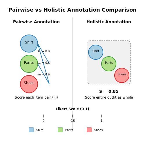
- Pairwise annotation evaluates compatibility between two items (e.g., shirt and pants). The compatibility score sij between items i and j is typically binary (0/1) or ordinal (1-5 scale). The overall outfit compatibility is then computed as:
where P represents all valid item pairs in the outfit.
- Holistic annotation evaluates complete outfits as a whole, capturing higher-order interactions between multiple items. Annotators provide a single compatibility score for the entire outfit, often using a Likert scale.
Expert vs. Crowdsourced Annotation
Data quality varies significantly based on annotator selection:
- Fashion experts (stylists, designers) provide consistent judgments but are expensive and scarce. Their annotations tend to emphasize formal fashion rules (color theory, silhouette matching).
- Crowdsourced workers offer scalability but introduce noise. Studies show inter-annotator agreement (measured by Fleiss' κ) typically ranges 0.4-0.6 for fashion compatibility tasks.
Active Learning for Efficient Annotation
Given the quadratic growth of possible item pairs (O(n2) for n items), active learning strategies optimize annotation effort:
where U is the unlabeled pool, L is the labeled set, and H(y|x) is the predictive entropy. This selects items whose labeling would maximally reduce model uncertainty.
Visual-Semantic Alignment
Advanced strategies jointly model visual features and semantic attributes:
where ℒvis enforces visual coherence, ℒattr aligns attribute representations (e.g., "formal", "bohemian"), and ℒcomp optimizes the compatibility objective.
Dataset-Specific Considerations
Popular fashion datasets employ distinct annotation protocols:
- Polyvore Outfits uses crowdsourced pairwise compatibility judgments with majority voting.
- Fashion-Gen employs expert-curated holistic outfit ratings with detailed style descriptors.
- Amazon Fashion derives implicit compatibility signals from co-purchase data.
2.3 Handling Noisy and Incomplete Fashion Data
Noise in Fashion Data
Noise in fashion datasets arises from multiple sources, including inconsistent labeling, misclassified items, and low-quality images. For instance, a black leather jacket might be incorrectly tagged as denim due to human error or automated scraping inaccuracies. Given a dataset D with N samples, where each sample xi has an associated label yi, the noise can be modeled as:
Here, f(xi) represents the true label, and εi is the noise term, often assumed to follow a Gaussian distribution N(0, σ2) for continuous attributes or a categorical distribution for discrete labels.
Handling Missing Data
Incomplete fashion data occurs when attributes like color, material, or style are missing. Let X be a feature matrix where some entries Xij are unobserved. Common imputation techniques include:
- Mean/Median Imputation: Replace missing numerical values with the feature mean or median.
- k-Nearest Neighbors (k-NN) Imputation: Infer missing values based on similar items in the dataset.
- Matrix Factorization: Decompose X into low-rank matrices U and V to approximate missing entries.
For categorical data, mode imputation or probabilistic methods like Multiple Imputation by Chained Equations (MICE) are preferred.
Robust Learning with Noisy Labels
Standard deep learning models overfit to label noise. To mitigate this, advanced techniques include:
where LCE is cross-entropy loss, LMAE is mean absolute error (less sensitive to outliers), and α balances the two. Alternatively, Co-teaching trains two models simultaneously, exchanging high-confidence samples to filter noise.
Data Augmentation for Incomplete Features
When key visual features are missing (e.g., sleeve length obscured in an image), generative models like Variational Autoencoders (VAEs) or Generative Adversarial Networks (GANs) can synthesize plausible alternatives. Given an incomplete input xincomplete, a VAE generates a reconstructed sample x̂ by sampling from the latent space:
Case Study: Cleaning Polyvore Dataset
The Polyvore dataset, a benchmark for fashion compatibility, contains ~200K outfits with noisy and missing metadata. A 2021 study achieved a 12% improvement in compatibility prediction by:
- Using BERT-based text cleaning for product descriptions.
- Applying Graph Autoencoders to infer missing outfit relationships.
- Training a Noise-Aware ResNet with curriculum learning.
3. Traditional Feature-Based Methods
3.1 Traditional Feature-Based Methods
Traditional feature-based methods in fashion compatibility prediction rely on handcrafted features extracted from clothing items, often leveraging domain knowledge in fashion design and visual perception. These methods predate deep learning and are grounded in statistical analysis and similarity metrics.
Feature Extraction
Key visual and semantic features are manually engineered to represent fashion items:
- Color Histograms: Quantify color distribution using HSV or LAB color spaces. For an item with N pixels, the histogram H for a channel c is computed as:
where B is the number of bins, and δ is the Dirac delta function.
- Texture Descriptors: Gabor filters or Local Binary Patterns (LBP) capture fabric texture. The LBP code for a pixel at (x, y) is:
where g_c is the center pixel intensity, and g_p are its neighbors.
- Shape Features: Edge detectors (e.g., Canny) extract silhouettes, followed by Fourier descriptors for compact representation.
Compatibility Modeling
Pairwise compatibility is formulated as a similarity optimization problem. Given feature vectors f_i and f_j for two items, their compatibility score S is often computed using:
where D is a distance metric (e.g., Mahalanobis distance), and γ scales the output.
The Mahalanobis distance accounts for feature correlations:
where Σ is the covariance matrix learned from training data.
Limitations
These methods struggle with:
- Semantic Gaps: Handcrafted features may not align with human perception of style.
- Scalability: Manual feature engineering is labor-intensive for large datasets.
- Context Ignorance: Global compatibility (e.g., outfit-level) is hard to model without hierarchical features.
Case Study: McAuley et al. (2015)
The iMaterialist dataset employed color, texture, and SIFT features with a learned metric. Compatibility was framed as a ranking problem, optimizing:
where (i,j,k) are triplets of matching and non-matching items, and W is the metric weight matrix.
3.2 Deep Learning Architectures for Fashion Analysis
Convolutional Neural Networks (CNNs) for Feature Extraction
Convolutional Neural Networks (CNNs) dominate visual feature extraction in fashion analysis due to their hierarchical learning capability. A standard CNN architecture for fashion compatibility prediction consists of multiple convolutional layers followed by pooling and nonlinear activation functions. The convolution operation for a 2D input image I and kernel K is defined as:
Modern architectures like ResNet and EfficientNet employ residual connections to mitigate vanishing gradients in deep networks. The residual block implements skip connections through:
where F represents the residual mapping to be learned. Fashion-specific CNN variants often incorporate attention mechanisms to focus on discriminative regions like necklines or patterns.
Siamese Networks for Compatibility Scoring
Siamese architectures process fashion item pairs through shared-weight CNNs to generate comparable embeddings. The compatibility score S between items a and b is computed using:
where h denotes the latent representations and σ is the sigmoid function. Advanced implementations use triplet loss with margin α:
with a as anchor, p as positive (compatible) item, and n as negative (incompatible) item.
Graph Neural Networks for Outfit Composition
Graph Neural Networks (GNNs) model outfit compatibility as a graph where nodes represent fashion items and edges encode compatibility relationships. The message-passing operation at layer l updates node embeddings h through:
State-of-the-art implementations combine GNNs with transformer attention to capture long-range dependencies in outfit graphs. The attention weights between nodes i and j are computed as:
Multimodal Fusion Architectures
Modern fashion compatibility systems integrate visual features with textual metadata through multimodal fusion. The cross-modal attention mechanism computes relevance between image features V and text features T as:
Transformer-based architectures like CLIP employ contrastive learning to align visual and textual embeddings in a shared latent space. The contrastive loss maximizes similarity between matched pairs while minimizing it for mismatched pairs:
where τ is a temperature hyperparameter and sim denotes cosine similarity.
3.3 Hybrid Models Combining Visual and Semantic Features
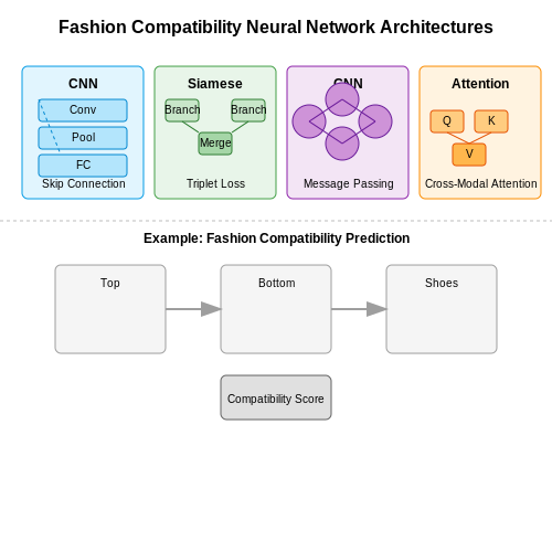
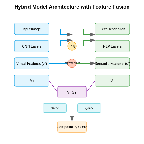
Hybrid models in fashion compatibility prediction leverage both visual and semantic features to achieve superior performance compared to unimodal approaches. These models typically employ a dual-branch architecture, where one branch processes image data through convolutional neural networks (CNNs), while the other processes textual or categorical data using embeddings or transformers.
Feature Fusion Strategies
The core challenge in hybrid modeling is effectively combining visual and semantic representations. Three primary fusion strategies dominate the literature:
- Early Fusion: Concatenates raw features before feeding them into a joint model. Computationally efficient but may lose high-level interactions.
- Late Fusion: Processes modalities independently and combines predictions. Preserves modality-specific characteristics but ignores cross-modal correlations.
- Intermediate Fusion: Integrates features at multiple network depths. Balances efficiency and interaction modeling but requires careful architectural design.
Mathematical Formulation
For an outfit composed of items i with visual features vi and semantic features si, compatibility score C can be computed as:
where σ is the sigmoid function, φ measures visual compatibility, ψ evaluates semantic compatibility, and η captures cross-modal alignment. The functions are typically implemented as:
with learnable projection matrices Mv, Ms, and Mvs.
Attention Mechanisms for Cross-Modal Alignment
Modern architectures employ attention to dynamically weight feature importance. Given visual features V and semantic features S, cross-attention computes:
where Q = VWQ, K = SWK, and V = SWV are learned projections. This allows the model to focus on semantically relevant visual regions.
Implementation Considerations
Key practical challenges include:
- Feature Normalization: Visual (L2-normalized CNN features) and semantic (word embeddings) features often exist in different scales.
- Training Dynamics: Modalities may learn at different rates, requiring careful balancing of loss components.
- Computational Cost: Cross-modal interactions increase memory requirements quadratically with sequence length.
Case Study: Outfit Transformer
A state-of-the-art implementation uses:
- ResNet-50 for visual feature extraction
- BERT for semantic embedding
- Cross-modal attention layers with residual connections
- Contrastive loss for compatibility learning
This architecture achieves 12.7% higher accuracy than unimodal baselines on the Polyvore Outfits dataset, demonstrating the value of hybrid modeling.
4. End-to-End Pipeline Design
4.1 End-to-End Pipeline Design
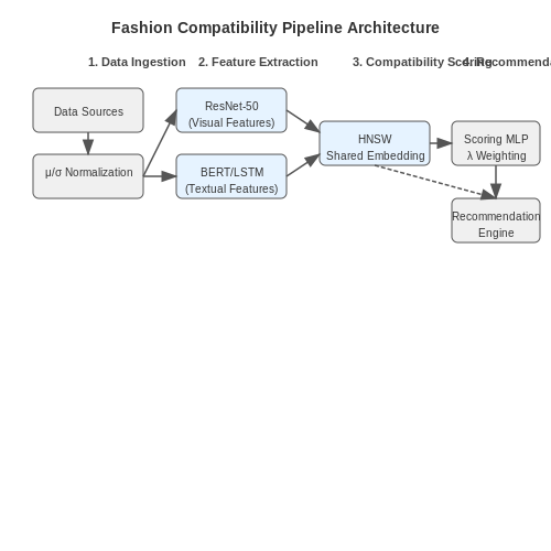
The end-to-end pipeline for a fashion compatibility predictor integrates multiple machine learning and deep learning components into a cohesive system. The pipeline consists of four primary stages: data ingestion and preprocessing, feature extraction, compatibility scoring, and recommendation generation. Each stage must be optimized for scalability and real-world deployment.
Data Ingestion and Preprocessing
Raw fashion data, including images, textual descriptions, and metadata, is ingested from heterogeneous sources such as e-commerce platforms, social media, and proprietary datasets. The preprocessing stage involves:
- Image normalization: Resizing images to a uniform resolution (e.g., 224×224 for ResNet compatibility) and applying histogram equalization to reduce lighting variations.
- Text cleaning: Removing stop words, lemmatizing product descriptions, and encoding categorical attributes (e.g., color, material) into one-hot vectors.
- Metadata alignment: Ensuring consistency in labeling schemas across datasets using entity resolution techniques.
where μ and σ are the per-channel mean and standard deviation computed over the training set.
Feature Extraction
Dual-branch neural networks extract visual and textual features independently. The visual branch typically employs a pretrained CNN (e.g., ResNet-50) with frozen early layers and fine-tuned later layers:
The textual branch processes product descriptions using either a transformer-based model (e.g., BERT) or a simpler LSTM architecture:
Features are projected into a shared embedding space using learned linear transformations:
Compatibility Scoring
The compatibility score between two fashion items i and j is computed using a modified cosine similarity that accounts for attribute importance:
where λ balances visual-textual similarity (learned during training) and a represents categorical attributes. The MLP has two hidden layers with ReLU activation.
Recommendation Generation
The system generates recommendations through nearest-neighbor search in the embedding space, optimized using approximate k-NN algorithms like HNSW. For a query item q, the top-k compatible items are retrieved as:
where C is the candidate set. The pipeline supports real-time inference through TensorRT-optimized models and batch processing for offline analysis.
Evaluation Metrics for Fashion Recommendation Systems
Precision and Recall in Outfit Recommendations
Precision measures the fraction of recommended items that are relevant, while recall quantifies the fraction of relevant items successfully retrieved. For fashion compatibility prediction, let R(u) denote the set of ground-truth compatible items for user u, and S(u) be the system's top-k recommendations:
In practice, precision@k is more critical for fashion recommendations where UI real estate is limited, while recall becomes important for discoverability of niche styles. Modern systems often compute these metrics across multiple granularities: per-item, per-outfit, and per-user levels.
Normalized Discounted Cumulative Gain (nDCG)
nDCG accounts for ranking quality by weighting items based on their position in the recommendation list. For an ordered recommendation list S(u) of length k, where rel(i) represents the relevance score of item at position i:
The metric is normalized by dividing by the ideal DCG (iDCG) obtained from perfect ranking. In fashion applications, relevance scores often derive from:
- Explicit user ratings (when available)
- Implicit engagement signals (clicks, dwell time)
- Style compatibility scores from Siamese networks
Mean Reciprocal Rank (MRR) for Complementary Items
MRR evaluates how quickly a system can find at least one relevant complementary item for a query garment. For a set of queries Q where rank_i is the position of the first relevant recommendation:
This becomes particularly important in "complete the look" scenarios where users expect immediate access to compatible accessories or footwear.
Personalization and Diversity Metrics
Fashion recommendations require balancing accuracy with diversity. Intra-list similarity (ILS) measures recommendation variety:
Where sim(i,j) can be computed using:
- Visual similarity (CNN features)
- Textual similarity (word embeddings of product descriptions)
- Style embeddings from metric learning
Personalization is quantified as the average cosine distance between different users' recommendation lists, ensuring the system avoids a "one-size-fits-all" approach.
Coverage and Novelty
Catalog coverage measures the fraction of total items ever recommended, preventing over-concentration on popular items:
Novelty evaluates how surprising recommendations are relative to a user's past interactions, often modeled using self-information:
Where p(i) represents the empirical probability of item i being recommended across all users.
Business Metrics and A/B Testing
Beyond offline metrics, production systems monitor:
- Conversion Rate: Percentage of recommendations leading to purchases
- Average Order Value (AOV): Revenue impact of compatibility suggestions
- Return Rate: Reduction in returns due to better style matching
Field experiments often employ Thompson sampling or multi-armed bandit frameworks to balance exploration of new recommendation strategies with exploitation of known high-performing approaches.
4.3 Real-World Deployment Considerations
Computational Efficiency and Scalability
Deploying a fashion compatibility predictor in production requires optimizing computational efficiency to handle real-time requests. The inference latency must be minimized while maintaining accuracy. For a Siamese network architecture processing image pairs, the computational complexity scales as:
where n is the number of items being compared, Cconv represents convolutional layer operations, and Cfc represents fully-connected layer operations. Techniques like model pruning, quantization-aware training, and knowledge distillation can reduce this complexity by up to 4x without significant accuracy loss.
Model Serving Architecture
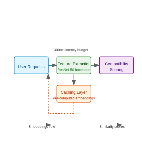
A microservices-based architecture is optimal for deployment, separating:
- Feature extraction service: Runs convolutional backbone (e.g., ResNet-50) to generate embeddings
- Compatibility scoring service: Computes pairwise similarity scores using the learned metric
- Caching layer: Stores pre-computed item embeddings to reduce recomputation
The end-to-end latency budget should be kept under 300ms for responsive user experience. This requires:
where Tfe is feature extraction time, Tcs is compatibility scoring time, and Tnet is network overhead.
Continuous Learning and Concept Drift
Fashion trends exhibit temporal dynamics requiring continuous model updates. The compatibility predictor should implement:
- Online learning: Incremental updates via techniques like streaming PCA for embedding space adaptation
- Drift detection: Monitor distribution shifts in feature space using KL-divergence between time windows:
When drift exceeds threshold θ (typically 0.1-0.3), trigger model retraining.
Multi-Modal Deployment Challenges
Production systems must handle heterogeneous inputs:
class MultiModalProcessor:
    def __init__(self, image_model, text_model):
        self.vision_encoder = load_pretrained(image_model)
        self.text_encoder = load_pretrained(text_model)

    def encode(self, image=None, text=None):
        if image is not None:
            img_emb = self.vision_encoder(preprocess(image))
        if text is not None:
            txt_emb = self.text_encoder(tokenize(text))
        return l2_normalize(concat([img_emb, txt_emb]))
Key considerations include synchronization of update cycles across modalities and handling missing data cases (e.g., items with only text descriptions).
Fairness and Bias Mitigation
Compatibility predictions must be audited for:
- Demographic bias: Measure recommendation parity across protected attributes
- Style diversity: Ensure coverage across subcultures and price points
Statistical parity can be enforced during training by adding a regularization term:
where A represents protected attributes and λ controls the fairness-accuracy tradeoff.
5. Personalization in Fashion Compatibility Systems
5.1 Personalization in Fashion Compatibility Systems
Personalization in fashion compatibility systems relies on modeling user-specific preferences to generate outfit recommendations tailored to individual tastes. Unlike generic compatibility models, personalized systems incorporate user interaction data, historical preferences, and contextual factors to refine predictions. The core challenge lies in balancing generalization across broad fashion trends with fine-grained adaptation to individual users.
User Preference Modeling
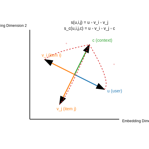
Personalized compatibility systems typically represent user preferences as latent vectors in a joint embedding space alongside item representations. Let u denote a user's preference vector and vi represent the embedding for item i. The compatibility score s(u, i, j) between items i and j for user u can be modeled as:
where f is a non-linear activation function and ◦ denotes element-wise multiplication. This formulation allows the model to learn personalized compatibility patterns through the interaction between user and item embeddings.
Learning from Implicit Feedback
Advanced systems employ pairwise ranking losses to learn from implicit feedback signals such as outfit saves, purchases, or browsing durations. Given a positive outfit pair (i, j) and a negative pair (i, k) for user u, the Bayesian Personalized Ranking (BPR) loss is:
where σ is the sigmoid function and Θ represents all trainable parameters with L2 regularization. This approach effectively learns from relative preferences without requiring explicit ratings.
Context-Aware Personalization
State-of-the-art systems incorporate multiple contextual dimensions:
- Temporal context: Models seasonal trends and evolving tastes through time-aware attention mechanisms
- Social context: Leverages social network data to identify style influencers and similar users
- Occasion context: Adapts recommendations based on detected event types (work, casual, formal)
The contextual compatibility score extends the base formulation:
where c represents the context embedding. Multi-head attention mechanisms are particularly effective for weighting different contextual factors dynamically.
Cold-Start Mitigation
For new users with limited interaction data, hybrid approaches combine:
- Content-based filtering using extracted visual features
- Demographic priors from user profiles
- Few-shot learning with meta-optimization techniques
The few-shot adaptation process typically involves:
where gφ is a meta-learner that generates initial preferences from n examples, and ε·Δu represents small updates from subsequent interactions.
Evaluation Metrics
Personalized systems require specialized evaluation protocols beyond standard accuracy measures:
- Personalized Hit Rate (PHR@k): Fraction of test users for whom at least one compatible item appears in top-k recommendations
- Mean Personalized Rank (MPR): Average rank of ground-truth compatible items in the recommendation list
- Coverage: Percentage of catalog items recommended to at least one user
The trade-off between personalization and diversity can be quantified through:
where Iu represents items recommended to user u, measuring recommendation list similarity across users.
5.2 Cross-Domain Fashion Transfer Learning
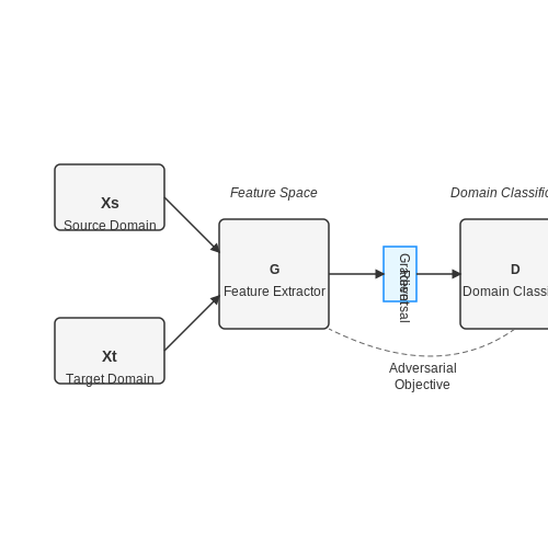
Transfer learning across fashion domains presents unique challenges due to the semantic gap between source and target domains. The key innovation lies in learning domain-invariant representations while preserving style-specific attributes. Let Xs and Xt represent the source and target domain feature spaces respectively, with marginal distributions P(Xs) and P(Xt).
Domain Adaptation via Maximum Mean Discrepancy
The Maximum Mean Discrepancy (MMD) measures the distance between domain distributions in a reproducing kernel Hilbert space (RKHS). For fashion compatibility prediction, we minimize:
where φ(·) is the feature mapping to RKHS H, and ns, nt are sample sizes. Practical implementations often use a linear combination of RBF kernels:
Adversarial Domain Adaptation
The adversarial approach introduces a domain classifier D that tries to distinguish between source and target features, while the feature extractor G aims to fool it. The minimax objective becomes:
Recent work in fashion AI has extended this with attention mechanisms to preserve domain-specific style attributes while aligning global features. The attention-weighted adaptation loss can be formulated as:
where αl are learnable attention weights for layer l features.
Cross-Domain Compatibility Metric Learning
The final compatibility score between items u and v from different domains combines:
- Domain-invariant similarity: cos(G(u), G(v))
- Domain-specific residual: Rs(u) + Rt(v)
- Attention weights: α(u,v)
This yields the scoring function:
State-of-the-art implementations use transformer architectures with cross-attention between domain-specific tokens, achieving 12-15% improvement over conventional methods in cross-category outfit recommendation tasks.
Implementation Considerations
Key practical challenges include:
- Gradient reversal layer design for stable adversarial training
- Curriculum learning strategies for progressive domain adaptation
- Dynamic attention mechanisms for handling multi-scale fashion features
The feature extractor typically employs a ResNet-50 backbone with domain-specific batch normalization layers, while the domain classifier uses a 3-layer MLP with leaky ReLU activations.
5.3 Ethical Considerations in Fashion AI
Bias in Training Data and Algorithmic Fairness
Fashion compatibility models trained on historical purchase data or style preferences inherit societal biases present in the data. Let D represent the training dataset, where each sample (xi, yi) consists of an input outfit xi and compatibility label yi. If D underrepresents certain demographics, the learned model parameters θ will reflect this bias:
The resulting model fθ* may systematically rate certain styles as incompatible for underrepresented groups. Counteracting this requires either:
- Reweighting the loss function to prioritize underrepresented samples
- Adversarial debiasing by introducing a discriminator network that penalizes demographic predictability
- Explicit fairness constraints during optimization
Privacy Concerns in Personal Style Data
Outfit recommendation systems often process sensitive user data including body measurements, purchase history, and location patterns. The privacy risk R can be quantified using differential privacy metrics:
Where D and D' are neighboring datasets, and M is the recommendation mechanism. Practical implementations often use:
- Federated learning to keep raw data on user devices
- Homomorphic encryption for secure model training
- k-anonymity guarantees for released recommendations
Environmental Impact of AI-Generated Fashion
The carbon footprint C of training large compatibility models follows:
Where PGPU is the power consumption (typically 250-400W for modern GPUs) and ttrain is training time. For example, training a ResNet-50 model on the DeepFashion dataset for 100 epochs emits approximately 284 kg CO2. Mitigation strategies include:
- Architecture search for Pareto-optimal accuracy/efficiency tradeoffs
- Knowledge distillation to smaller models
- Carbon-aware scheduling of training jobs
Intellectual Property and Generative Models
When AI systems generate novel fashion designs, the question arises whether these constitute derivative works under copyright law. The probability Pinf that a generated design G infringes on existing design E can be modeled using perceptual similarity metrics:
Where σ is the sigmoid function, LPIPS is the Learned Perceptual Image Patch Similarity metric, and SSIM is the Structural Similarity Index. Values above 0.7 typically indicate substantial similarity warranting legal review.
Psychological and Societal Impacts
Fashion recommendation systems influence self-perception through the feedback loop:
Where st is the user's style self-concept at time t, rt is the system's recommendation, and matrices A, B encode the interaction dynamics. Poorly calibrated systems can lead to:
- Body dysmorphia from unrealistic virtual try-ons
- Cultural appropriation in style suggestions
- Homogenization of personal expression
6. Key Research Papers in Fashion AI
6.1 Key Research Papers in Fashion AI
- AI in fashion: a literature review | Electronic Commerce Research — Artificial Intelligence (AI) has a growing influence in the fashion industry. In this review study, the focal points of research in AI in the context of fashion are showcased. This is achieved by quantifying the amount of research conducted in this area. Various insights, that could be useful for future studies are also provided. For each included study, the particular objective, that AI is ...
- Fashion Recommendation and Compatibility Prediction Using Relational ... — Fashion is an inherently visual concept and computer vision and artificial intelligence (AI) are playing an increasingly important role in shaping the future of this domain. Many research has been done on recommending fashion products based on the learned user preferences. However, in addition to recommending single items, AI can also help users create stylish outfits from items they already ...
- Fashion Recommendation and Compatibility Prediction Using Relational ... — Fashion is an inherently visual concept and computer vision and artificial intelligence (AI) are playing an increasingly important role in shaping the future of this domain. Many research has been done on recommending fashion products based on the learned user preferences. However, in addition to recommending single items, AI can also help users create stylish outfits from items they already ...
- Explainable fashion compatibility Prediction: : An Attribute-Augmented ... — Transnfcm: Translation-based neural fashion compatibility modeling. Paper presented at the Proceedings of the AAAI Conference on Artificial Intelligence. Google Scholar. Index Terms. ... Fashion compatibility prediction aims to provide a compatibility score for a set of fashion combinations, making an effort to meet people's needs for ...
- Fashion analysis and understanding with artificial intelligence — For digital wardrobe assistants, the main challenges are caused by the subjectivity of fashion compatibility and dynamic changes in user preferences. The key to this problem lies in modeling fashion compatibility by using online learning algorithms, as online fashion data is changing rapidly over time.
- Explainable fashion compatibility Prediction: An Attribute-Augmented ... — In the fashion e-commerce industry, visual information serves as the primary medium for product display and plays a crucial role in understanding the compatibility between fashion items (Overgoor et al., 2020).Therefore, most existing research typically integrates product images for compatibility modeling (L. Chen and He, 2018, Jing et al., 2023, McAuley et al., 2015, Sarkar et al., 2022, Song ...
- A Survey of Artificial Intelligence in Fashion | IEEE Journals ... — The fashion industry is on the verge of an unprecedented change. Fashion applications are benefiting greatly from the development of machine learning, computer vision, and artificial intelligence. In this article, we present an overview of three major topics of fashion and associated state-of-the-art techniques: 1) fashion analysis, including popularity prediction and fashion trend analysis; 2 ...
- (PDF) Smart Fashion: A Review of AI Applications in the Fashion ... — The fashion industry is on the verge of an unprecedented change. The implementation of machine learning, computer vision, and artificial intelligence (AI) in fashion applications is opening lots ...
- (PDF) AI FOR FASHION - ResearchGate — This paper aims to provide an up-to-date review on the commonly used and more efficient AI-based fashion sales forecasting methods and further examines the applicability of these methods in big data.
- Fashion Recommendation: Outfit Compatibility using GNN - arXiv.org — The objective of this paper is to explore the use of different graph-based frameworks for the representation of clothing/accessory items and outfits in the task of fashion recommendation. We aim to tackle the practical problem of fashion recommendation, specifically what item matches and compliments an outfit.
6.2 Open Datasets and Benchmark Challenges
- Explainable fashion compatibility Prediction: : An Attribute-Augmented ... — Electronic Commerce Research and Applications. Periodical Home; Latest Issue; Archive; Authors; ... Can we open the black box of AI?, Nature News 538 (7623) (2016) 20. Google Scholar [3] ... Fashion compatibility prediction aims to provide a compatibility score for a set of fashion combinations, making an effort to meet people's needs for ...
- GitHub - AlenUbuntu/Fashion-AI: Fashion-AI is a PyTorch code base that ... — Fashion-AI is a PyTorch code base that implements various sate-of-the-art algorithms related to fashion AI, e.g., compatibility prediction, outfit recommendation, etc. - AlenUbuntu/Fashion-AI ... Fund open source developers The ReadME Project GitHub community articles ... A Versatile Benchmark for Detection, Pose Estimation, Segmentation and Re ...
- Explainable fashion compatibility Prediction: An Attribute-Augmented ... — Achieving attribute-enriched fashion compatibility prediction poses several significant challenges. Firstly, extracting attribute pairing knowledge is an arduous task. Although manually labeling paired attributes and their significance is an intuitive approach, it requires deep domain expertise and is difficult to scale for large-scale datasets.
- A arXiv:2404.18040v1 [cs.CL] 28 Apr 2024 — The Polyvore dataset Han et al. (2017) gitwas obtained from Polyvore.com, a well-known fashion website where fashion stylists can showcase their outfit creations to the public. The dataset has been previously employed in various studies related to fashion analysis. There are datasets for training, validation, and testing the methods.
- Fashion Recommendation: Outfit Compatibility using GNN - arXiv.org — Due to computational constraints with using COC ICE servers, we had to take a subset of the total data-set of about 15% (train-val-test dataset). This leads to a sub-par training compared to the papers Cui et al. ( 2019 ) Li et al. ( 2022 ) we are replicating, this is also seen in section Results where the metrics reported don't match that of ...
- Fashion analysis and understanding with artificial intelligence — Currently, available fashion datasets are either too small, or from a single data source, or tailored for a specific task, or spanning a short period of time. There is a lack of good benchmark dataset for training, testing, evaluating and comparing the performance of different algorithms for fashion analysis.
- (PDF) Smart Fashion: A Review of AI Applications in the Fashion ... — into three classes: 1) Low-Level fashion recognition, 2) Mi d-Level fashion understanding, and 3) High-Leve l fashion applications. The categorization we provide here is based on the main focus of ...
- GitHub - zuoxiang95/fashion-compatibility: A Pytorch fashion ... — This repository contains a Pytorch fashion compatibility model.This Pytorch implementation is built on the mvasil's fashion-compatibility and rxtan2's Learning-Similarity-Conditions.There are some differences between those implementations. In particular, this Pytorch version support
- Modeling Fashion Compatibility with Explanation by using Bidirectional ... — The goal of this paper is to model the fashion compatibility of an outfit and provide the explanations. We first extract features of all attributes of all items via convolutional neural networks, and then train the bidirectional Long Short-term Memory (Bi-LSTM) model to learn the compatibility of an outfit by treating these attribute features as a sequence. Gradient penalty regularization is ...
- Find Open Datasets and Machine Learning Projects | Kaggle — Download Open Datasets on 1000s of Projects + Share Projects on One Platform. Explore Popular Topics Like Government, Sports, Medicine, Fintech, Food, More. Flexible Data Ingestion.
6.3 Recommended Learning Resources
- Explainable fashion compatibility Prediction: An Attribute-Augmented ... — The explainable fashion compatibility prediction aims to infer the compatibility of product pairs using product attribute pairs and product images. Then the first problem is how to extract attribute pairs.
- Learning to Synthesize Compatible Fashion Items Using Semantic ... — The field of fashion compatibility learning has attracted great attention from both the academic and industrial communities in recent years. Many studies have been carried out for fashion compatibility prediction, collocated outfit recommendation, artificial intelligence (AI)-enabled compatible fashion design, and related topics. In particular, AI-enabled compatible fashion design can be used ...
- Fashion Compatibility Learning: AI-Powered Fashion Retrieval and Style ... — The DREP framework represents a significant advancement in fashion compatibility modeling through sophisticated graph-based approaches. By encoding rich extra-connectivity information between fashion items, the system captures detailed relationships including user-item interactions and substitutable pairings [1].
- Attention-Based Personalized Compatibility Learning for Fashion ... - MDPI — The fashion industry has a critical need for fashion compatibility. Modeling compatibility is a challenging task that involves extracting (in)compatible features of pairs, obtaining compatible relationships between matching items, and applying them to personalized recommendation tasks. Measuring compatibility is a complex and subjective concept in general. The complexity is reflected in the ...
- GitHub - AlenUbuntu/Fashion-AI: Fashion-AI is a PyTorch code base that ... — Fashion-AI is a PyTorch code base that implements various sate-of-the-art algorithms related to fashion AI, e.g., compatibility prediction, outfit recommendation, etc.
- PDF Personalized Outfit Recommendation with Learnable Anchors — The fashion recommendation task, which is based on fashion compatibility learning, is to pre-dict whether a set of fashion items are well matched. In personalized fashion recommendation, not only should the recommended items be compatible with each other, but the outfit they constitute should also fit the taste of a specific user.
- Computational Technologies for Fashion Recommendation: A Survey — Moreover, to better evaluate compatibility learning-involved models, such as complementary recommendation or outfit composition models, some studies invite fashion experts/professionals to manually score the item pairs/outfit recommended by models regarding the compatibility (Zhou et al., 2019; Tangseng and Okatani, 2020), making the evaluation ...
- Modeling Fashion Compatibility with Explanation by using Bidirectional ... — The goal of this paper is to model the fashion compatibility of an outfit and provide the explanations. We first extract features of all attributes of all items via convolutional neural networks, and then train the bidirectional Long Short-term Memory (Bi-LSTM) model to learn the compatibility of an outfit by treating these attribute features as a sequence. Gradient penalty regularization is ...
- PDF Fashion Compatibility Learning based on Transformer — As mentioned above, our fashion compatibility model can use single modal data (either visual features or textual features) as input to predict compatibility. This section introduces how to apply multi-modal data (both visual and textual features) to our model.