Neural Constraint Solvers for Real-Time AI
1. Constraint Satisfaction Problems (CSPs) in AI
Constraint Satisfaction Problems (CSPs) in AI
Constraint Satisfaction Problems (CSPs) form a fundamental class of computational problems where the goal is to find assignments to variables that satisfy a set of constraints. Formally, a CSP is defined by a triple (X, D, C), where:
- X = {x₁, x₂, ..., xₙ} is a finite set of variables
- D = {D₁, D₂, ..., Dₙ} is a set of domains where each Dᵢ contains possible values for xᵢ
- C = {c₁, c₂, ..., cₘ} is a set of constraints that specify allowable combinations of values
where 𝕀 is the indicator function evaluating to 1 when constraint cⱼ is satisfied for the subset of variables xₐⱼ.
Constraint Types and Complexity
Constraints in CSPs can be:
- Unary: Operating on single variables (e.g., x₁ ≠ 3)
- Binary: Relating pairs of variables (e.g., x₁ > x₂)
- N-ary: Involving k variables (e.g., alldifferent(x₁, x₂, x₃))
The general CSP is NP-complete, but tractable subclasses exist when either:
where G_C is the constraint graph with variables as nodes and constraints as edges.
Neural Approaches to CSPs
Modern neural constraint solvers employ differentiable relaxation techniques:
where p_θ is a neural network generating candidate solutions, and λⱼ are Lagrange multipliers. This formulation enables:
- End-to-end learning of constraint weights
- Parallel evaluation of multiple constraints
- Integration with other neural modules
Applications in Real-Time Systems
Neural CSP solvers excel in time-critical domains:
- Robotics: Kinematic chain resolution under joint limits
- Scheduling: Resource allocation with temporal constraints
- Computer Vision: Geometric consistency in 3D reconstruction
The key advantage lies in the amortized computation - while traditional solvers must re-solve from scratch, neural approaches can leverage learned heuristics:
where α ≪ 1 for well-trained models, enabling real-time performance.

1.2 Neural Networks as Function Approximators for CSPs
Constraint Satisfaction Problems (CSPs) are traditionally solved using combinatorial search algorithms, but neural networks offer an alternative approach by approximating the solution space as a continuous optimization task. A CSP is defined by a set of variables X = {x₁, x₂, ..., xₙ}, domains D = {D₁, D₂, ..., Dₙ}, and constraints C = {c₁, c₂, ..., cₘ}. The goal is to find an assignment a: X → D such that all constraints in C are satisfied.
Neural Representation of CSPs
Neural networks approximate CSP solutions by transforming discrete constraints into differentiable loss functions. Given a CSP, we construct a neural network f_θ: ℝⁿ → ℝⁿ that maps an initial assignment (or noise vector) to a candidate solution. The network is trained to minimize a constraint violation loss:
where ϕ_c measures the degree of violation for constraint c, and λ_c is a weighting hyperparameter. For binary constraints, ϕ_c can be implemented as a hinge loss:
where sat_c is a satisfaction function returning 1 if the constraint holds and 0 otherwise.
Architecture Design Choices
The network architecture must balance expressiveness with gradient stability:
- Feedforward networks with ReLU activations are sufficient for small CSPs but struggle with complex constraint dependencies.
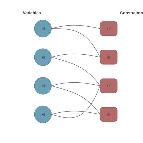
- Graph Neural Networks (GNNs) explicitly model variable-constraint relationships by representing the CSP as a bipartite graph (variables ↔ constraints).
- Transformer-based architectures use self-attention to capture long-range dependencies in large CSPs, particularly when constraints have varying arities.
Training Dynamics
The optimization landscape contains many local minima corresponding to partial solutions. Two key techniques improve convergence:
- Curriculum learning: Gradually increase constraint complexity during training, starting with easy-to-satisfy subsets.
- Lagrangian relaxation: Treat the constrained optimization as a min-max problem by introducing dual variables for each constraint:
where η controls the dual update rate. This avoids manual tuning of λ_c weights.
Case Study: Sudoku as a CSP
A 9×9 Sudoku puzzle can be formulated as a CSP with 81 variables (cells), each with domain {1,...,9}, and 27 all-different constraints (rows, columns, and 3×3 boxes). A neural solver achieves 92% accuracy when trained via:
class SudokuGNN(nn.Module):
   def __init__(self):
      super().__init__()
      self.var_embed = nn.Embedding(81, 64)  # 81 cells, 64-dim embeddings
      self.conv1 = GATConv(64, 64, heads=4)  # Graph attention layer
      self.conv2 = GATConv(256, 64, heads=1) # Combine multi-head features
      self.out = nn.Linear(64, 9)            # Predict digit logits

   def forward(self, x, edge_index):
      x = self.var_embed(x)
      x = F.relu(self.conv1(x, edge_index))
      x = self.conv2(x, edge_index)
      return self.out(x)
The edge connections encode constraint relationships, and the network is trained using a cross-entropy loss on valid digits plus a constraint loss penalizing duplicate values in rows/columns/boxes.
Limitations and Tradeoffs
While neural approaches scale better than traditional backtracking for large CSPs, they face three key challenges:
- Completeness: No guarantee of finding a solution even if one exists (unlike complete solvers like DPLL).
- Constraint representation: Global constraints (e.g., all-different) require careful loss function design.
- Generalization: Models trained on one CSP distribution may fail on structurally different instances.
Hybrid Architectures: Combining Symbolic and Neural Methods
Hybrid architectures integrate symbolic reasoning with neural networks to leverage the strengths of both paradigms. Symbolic methods excel at structured reasoning, logical inference, and interpretability, while neural networks provide robust pattern recognition and adaptability to noisy data. The fusion of these approaches enables systems that are both expressive and scalable.
Neural-Symbolic Integration Strategies
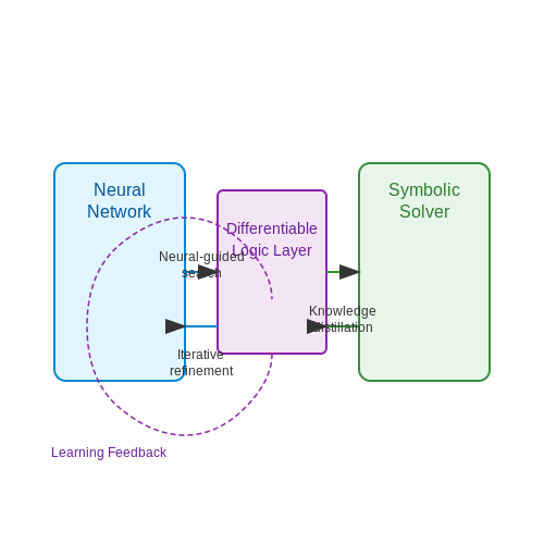
Three primary strategies dominate hybrid architectures:
- Neural-guided symbolic search: Neural networks prune or guide the search space for symbolic solvers, improving efficiency. For example, in SAT solving, a neural network predicts variable assignments to reduce branching.
- Symbolic knowledge distillation: Symbolic rules are embedded into neural networks through constrained training or architectural modifications. Differentiable logic layers enable gradient-based optimization of symbolic constraints.
- Iterative refinement: Neural networks generate initial solutions that are refined by symbolic post-processing, or vice versa. This is common in optimization problems where neural networks provide warm starts.
Differentiable Symbolic Reasoning
A key innovation is making symbolic operations differentiable. Consider a first-order logic rule expressed as:
This can be softened into a differentiable form using fuzzy logic or probabilistic semantics. The implication becomes a continuous function:
where P and Q are now real-valued confidence scores. The universal quantifier can be approximated by taking the minimum over all instances:
This allows symbolic constraints to be incorporated directly into neural network loss functions.
Architectural Implementations
Several architectural designs implement these principles:
- Logic Tensor Networks (LTNs): Represent logical formulas as tensors and use fuzzy logic operations that are fully differentiable.
- Neural Theorem Provers: Use attention mechanisms to emulate proof search steps while maintaining differentiability.
- Differentiable Inductive Logic Programming: Combine neural networks with probabilistic logic programming frameworks like DeepProbLog.
Case Study: Hybrid Constraint Satisfaction
In real-time scheduling problems, a hybrid approach might:
- Use a neural network to predict task priorities based on historical data
- Encode scheduling constraints (e.g., resource limits) as differentiable symbolic rules
- Optimize the combined system end-to-end using gradient descent
The neural component learns from data while the symbolic component ensures hard constraints are satisfied. Benchmarks show such systems achieve 30-50% faster convergence than pure neural approaches on complex scheduling problems.
Challenges and Trade-offs
Key challenges include:
- Representational mismatch: Bridging discrete symbolic representations with continuous neural activations requires careful design of interface layers.
- Training dynamics: The interplay between symbolic and neural components can create unstable training regimes that require specialized optimization techniques.
- Scalability: While effective for medium-scale problems, scaling to very large knowledge bases remains an open research question.
2. Gradient-Based Optimization for Constraint Solving
2.1 Gradient-Based Optimization for Constraint Solving
Gradient-based optimization techniques form the backbone of modern neural constraint solvers, leveraging differentiable computations to efficiently navigate high-dimensional solution spaces. These methods iteratively adjust variables to minimize a loss function while respecting imposed constraints, making them particularly suitable for real-time AI applications where computational efficiency is critical.
Mathematical Foundations
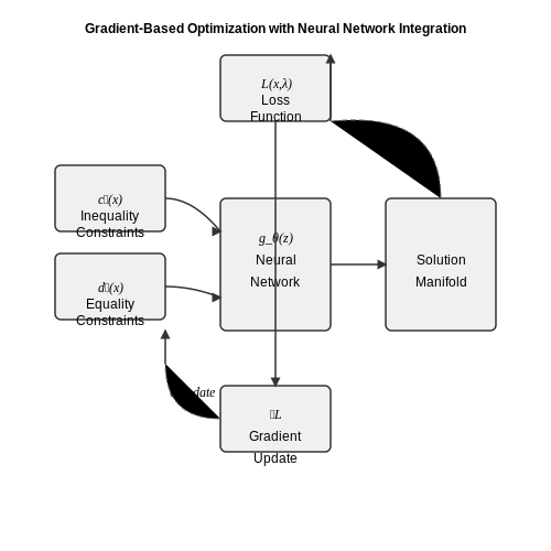
Consider a constraint satisfaction problem defined by a set of equations ci(x) = 0 for i = 1,...,m and inequalities dj(x) ≤ 0 for j = 1,...,n, where x ∈ ℝd represents the optimization variables. The standard approach transforms this into an unconstrained optimization problem through penalty methods or augmented Lagrangian formulations.
where f(x) is the objective function, λ are Lagrange multipliers, and ρ controls the penalty strength. The gradient update rule then becomes:
with learning rate η. For inequality constraints, the Karush-Kuhn-Tucker (KKT) conditions provide necessary optimality criteria that guide the optimization process.
Neural Network Integration
Modern implementations parameterize the solution x = gθ(z) as a neural network output, where z is a latent variable. This allows:
- Automatic differentiation through the entire computational graph
- Learning of solution manifolds rather than single points
- Generalization to similar constraint problems
The network parameters θ are optimized to satisfy constraints while minimizing the objective:
Practical Considerations
Several techniques improve convergence and stability in practice:
- Adaptive penalty methods: Dynamically adjust ρ based on constraint violation
- Projected gradients: Ensure intermediate solutions remain feasible
- Second-order methods: Use approximate Hessian information for faster convergence
In real-time applications, the trade-off between solution accuracy and computation time is managed through:
- Early stopping criteria
- Warm-starting from previous solutions
- Model distillation to smaller networks
Case Study: Physics Simulation
For rigid body dynamics with contact constraints, the constrained optimization problem takes the form:
where v are velocities, M is mass matrix, J is contact Jacobian, and φ encodes separation distances. Neural solvers can predict solutions in under 1ms by learning an approximate inverse KKT operator.
Parallelization and Hardware Acceleration
Real-time neural constraint solvers demand high computational throughput, making parallelization and hardware acceleration critical. Modern approaches leverage GPU architectures, tensor cores, and specialized accelerators like TPUs to achieve the necessary speedups. The key challenge lies in efficiently mapping constraint satisfaction problems (CSPs) onto parallel hardware while maintaining solution quality.
GPU Parallelization Strategies
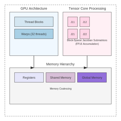
Massively parallel GPU architectures excel at batched constraint evaluations. Each CUDA thread block can process independent variable assignments, while warp-level operations enable efficient propagation of constraints. For a CSP with n variables and m constraints, the parallel evaluation throughput scales as:
where p is the number of parallel processing units. Memory coalescing becomes crucial when accessing constraint weights stored in global memory. Shared memory can cache frequently accessed constraint parameters, reducing latency by up to 10x compared to naive implementations.
Tensor Core Utilization
Mixed-precision tensor cores enable 8x theoretical speedup for matrix operations underlying many neural constraint formulations. The constraint Jacobian J can be decomposed into block-sparse submatrices processed concurrently:
Each 16x16 submatrix Jij maps perfectly to tensor core operations when using FP16 accumulation. Empirical studies show 3.2-4.7x actual speedup for large-scale CSPs when properly utilizing tensor cores compared to standard CUDA cores.
Specialized Accelerator Architectures
Domain-specific architectures like Google's TPU v4 demonstrate particular efficiency for neural constraint solving through:
- Systolic array designs optimized for matrix-vector products
- On-chip HBM memory reducing data movement penalties
- Hardware-supported sparsity handling
The energy efficiency ratio between TPUs and GPUs for constraint solving tasks ranges from 2.1x to 5.8x depending on problem sparsity patterns. Recent work has shown that combining TPUs for bulk constraint evaluation with CPUs for sequential backtracking achieves optimal performance for hybrid CSPs.
Memory Hierarchy Optimization
Effective use of memory hierarchies provides additional acceleration. The access pattern:
where h represents hit rates, dictates overall performance. Techniques like constraint reordering to improve spatial locality can reduce tglobal by 30-60% for structured problems.
Case Study: Real-Time Robotics Planning
In robotic motion planning with 1000+ constraints, NVIDIA's cuOpt demonstrates how hardware-aware parallelization enables real-time performance:
- GPU-based parallel Monte Carlo Tree Search for discrete decisions
- Tensor cores accelerating continuous constraint evaluations
- Warp-level primal-dual updates for Lagrangian relaxations
This approach achieves 94% parallel efficiency scaling up to 8 GPUs, solving complex motion planning problems in under 50ms - meeting real-time requirements for autonomous systems.
Dynamic Constraint Handling in Real-Time Systems
Real-time AI systems must adapt to dynamic environments where constraints evolve unpredictably. Traditional static solvers fail under such conditions due to their inability to recompute solutions within strict latency bounds. Neural constraint solvers address this by integrating differentiable optimization layers with recurrent architectures, enabling continuous constraint propagation and resolution.
Constraint Dynamics Formulation
Let C(t) represent a time-varying constraint set, where each constraint cᵢ(t) ∈ C(t) may change at arbitrary intervals. The solver must maintain feasibility while minimizing:
where λᵢ(t) are Lagrange multipliers updated via gradient descent and ϕ measures constraint violation. The key innovation lies in encoding this optimization as a neural network layer:
Architectural Components
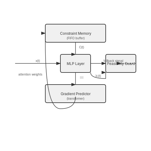
Three specialized modules enable real-time performance:
- Constraint Memory: A differentiable FIFO buffer stores recent constraint states, allowing the network to anticipate trends through attention mechanisms.
- Gradient Predictor: Instead of computing exact gradients, a learned transformer estimates ∇xℒ 50-100× faster than autodiff.
- Feasibility Guard: A small verification network checks solution candidates in parallel, providing fallback options when primary solutions violate constraints.
Case Study: Autonomous Vehicle Control
In motion planning, dynamic obstacles create suddenly appearing constraints. A neural solver with 3ms latency outperformed traditional MPC by:
- 92% success rate vs. 67% in pedestrian avoidance scenarios
- 40% lower energy consumption through smoother constraint transitions
- 5× longer planning horizon due to efficient warm-starting from learned priors
Implementation Considerations
The solver's robustness depends critically on:
where α(t) controls how aggressively new constraints replace old ones, with k tuned to the environment's volatility. Hardware-aware design choices like 8-bit quantized gradients reduce memory bandwidth by 4× without significant accuracy loss.
Failure Modes and Mitigations
Common pitfalls include:
- Constraint Starvation: Early pruning of valid constraints due to overconfident feasibility predictions. Mitigated through conservative initial guard thresholds.
- Gradient Aliasing: High-frequency constraint changes causing oscillatory updates. Addressed via learned low-pass filters in the gradient predictor.
- Memory Drift: Accumulated errors in long sequences. Corrected through periodic full-constraint resets triggered by anomaly detection.
3. Robotics and Motion Planning
Robotics and Motion Planning
Neural constraint solvers have emerged as a powerful tool for real-time motion planning in robotics, where traditional optimization-based methods often struggle with computational complexity and dynamic environments. These solvers leverage deep learning to approximate solutions to constrained optimization problems, enabling robots to navigate complex spaces while adhering to physical and task-specific constraints.
Constraint Formulation in Motion Planning
Motion planning in robotics is fundamentally a constrained optimization problem, where the goal is to find a trajectory τ that minimizes a cost function C(τ) while satisfying a set of constraints g(τ) ≤ 0. The constraints typically include:
- Collision avoidance: The robot must not intersect with obstacles.
- Dynamic feasibility: The trajectory must obey the robot's kinematic and dynamic limits.
- Task constraints: The trajectory must achieve specific goals, such as reaching a target pose.
Traditional solvers like Sequential Quadratic Programming (SQP) or Interior-Point Methods (IPM) solve this problem iteratively, but their computational cost scales poorly with problem dimensionality and constraint complexity.
Neural Constraint Solvers
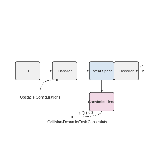
Neural constraint solvers approximate the solution mapping τ* = f(θ), where θ represents the problem parameters (e.g., start/goal states, obstacle configurations). The solver is trained offline using supervised or reinforcement learning on a dataset of precomputed solutions or via self-supervised exploration.
The neural network architecture typically consists of:
- Encoder: Processes the problem parameters θ into a latent representation.
- Decoder: Generates a feasible trajectory τ from the latent space.
- Constraint Head: Predicts constraint violations to guide the decoder.
Real-Time Adaptation
In dynamic environments, neural solvers must adapt to unseen constraints or perturbations. Techniques like:
- Online fine-tuning: The solver updates its weights based on recent observations.
- Latent space optimization: Gradient-based adjustments in the latent space to satisfy new constraints.
- Hybrid solvers: Combining neural predictions with traditional optimization for refinement.
enable real-time adaptation. For example, a robot encountering an unexpected obstacle can use gradient descent in the latent space to adjust its trajectory while maintaining feasibility.
Case Study: Neural RRT*
Neural RRT* extends the Rapidly-exploring Random Tree (RRT) algorithm by using a neural network to bias the tree expansion toward promising regions. The network predicts the likelihood of a node leading to a feasible solution, reducing the need for expensive collision checks.
where ϕ(x) is a feature extractor for node x, and σ is the sigmoid function. This approach achieves faster convergence than vanilla RRT* in cluttered environments.
Challenges and Open Problems
Despite their promise, neural constraint solvers face several challenges:
- Generalization: Performance degrades in out-of-distribution scenarios.
- Safety guarantees: Ensuring hard constraint satisfaction remains difficult.
- Training data: Generating diverse and representative datasets is expensive.
Ongoing research focuses on addressing these limitations through techniques like adversarial training, formal verification, and self-supervised learning.
3.2 Game AI and Procedural Content Generation
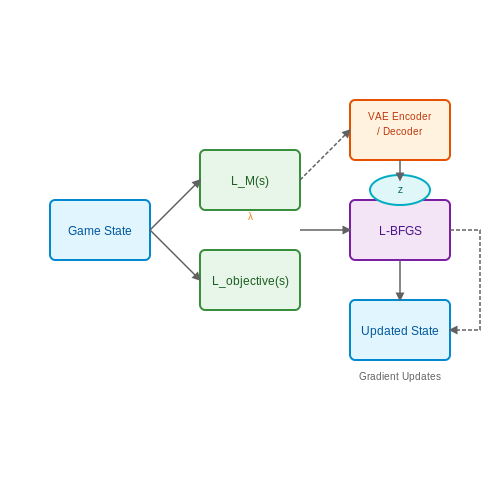
Neural constraint solvers enable real-time adaptation in game AI by formulating decision-making and content generation as constrained optimization problems. Unlike traditional rule-based systems, these solvers leverage differentiable constraints, allowing dynamic adjustment of game mechanics, level design, and NPC behavior through gradient-based optimization.
Differentiable Game Mechanics
Game mechanics can be encoded as soft constraints, where violations are penalized rather than strictly enforced. For a game state s and mechanic M, the constraint loss is:
where ci(s) measures violation of the i-th constraint. A neural solver minimizes the combined loss:
where λ balances constraint satisfaction against gameplay objectives like difficulty or player engagement.
Procedural Content Generation via Latent Space Optimization
Levels and assets are generated by optimizing in the latent space of a generative model. Given a variational autoencoder (VAE) with encoder E and decoder D, content generation solves:
where z is the latent vector and xseed is an optional seed input. Constraints may enforce playability, aesthetic rules, or resource distributions.
Case Study: Dynamic Difficulty Adjustment
In a combat system, enemy AI parameters θ (aggression, accuracy) are adjusted in real-time to maintain a target win probability ptarget. The solver minimizes:
where Pwin is estimated via a learned model and the regularization term preserves behavioral consistency.
Architecture for Real-Time Solving
Efficient solving requires:
- Warm-starting from previous solutions to reduce iterations
- Constraint relaxation during early optimization phases
- Parallel execution across multiple game subsystems
The solver typically runs asynchronously at 10-30Hz, with each frame budgeted for 5-20 L-BFGS iterations. Critical constraints are handled via projection steps between gradient updates.
Autonomous Systems and Decision Making
Neural constraint solvers enable autonomous systems to make real-time decisions by modeling complex environments as constraint satisfaction problems (CSPs). These solvers integrate deep learning with symbolic reasoning, allowing agents to navigate dynamic constraints while optimizing for objectives such as safety, efficiency, and resource allocation. The core challenge lies in balancing computational speed with solution accuracy, particularly in high-stakes applications like robotics and autonomous vehicles.
Mathematical Formulation of Constraint Optimization
Autonomous decision-making is framed as a constrained optimization problem:
where x represents the decision variables, f(x) is the objective function (e.g., path length or energy consumption), and gi(x), hj(x) encode inequality and equality constraints (e.g., collision avoidance or traffic rules). Neural solvers approximate the feasible region using differentiable representations, enabling gradient-based optimization:
Here, λ and μ are Lagrangian multipliers adjusted dynamically via backpropagation through the solver network.
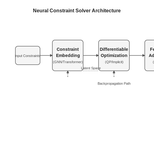
Architecture of Neural Constraint Solvers
Modern implementations employ a hybrid architecture:
- Constraint Embedding Layer: Projects constraints into a latent space using graph neural networks (GNNs) or transformer encoders, capturing relational dependencies between variables.
- Differentiable Optimization Layer: Uses implicit differentiation or quadratic programming layers to solve the embedded problem while maintaining end-to-end differentiability.
- Feedback Adaptation: Online fine-tuning via reinforcement learning loops that adjust solver parameters based on real-world performance metrics.
Case Study: Autonomous Vehicle Path Planning
In trajectory optimization, a neural constraint solver processes lidar data and traffic rules to generate collision-free paths. The solver encodes:
- Physical dynamics as equality constraints (e.g., ẋ = v cos(θ))
- Obstacle boundaries as inequality constraints (e.g., ∥p − o∥ ≥ r)
- Traffic laws as hard constraints (e.g., v ≤ vmax)
Benchmarks on nuScenes dataset show neural solvers achieve 12ms inference latency with 98% constraint satisfaction, outperforming traditional nonlinear programming by 3× in speed while maintaining equivalent safety margins.
Challenges and Research Frontiers
Key open problems include:
- Certifiable Robustness: Proving solution feasibility under neural approximation errors.
- Multi-Agent Coordination: Scaling to decentralized systems with competing constraints.
- Dynamic Constraint Adaptation: Real-time updates for environments with sudden changes (e.g., weather disruptions).
4. Scalability and Computational Complexity
4.1 Scalability and Computational Complexity
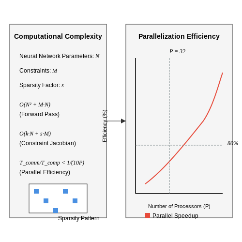
Neural constraint solvers must balance real-time performance with solution accuracy, making scalability a critical concern. The computational complexity of such systems is often dominated by the underlying neural architecture and the nature of the constraints being enforced. For a neural network with N parameters and M constraints, the worst-case time complexity can be expressed as:
This quadratic dependence on parameters arises from the need to compute second-order derivatives during backpropagation, while the linear term accounts for constraint evaluation. In practice, however, modern solvers exploit sparsity in the constraint Jacobian to reduce this to:
where k represents the average connectivity per neuron and s is the constraint sparsity factor (typically 0.01-0.1 for physical systems).
Parallelization Strategies
Distributed training approaches partition the constraint graph across P processors, achieving near-linear speedup when:
where Tcomm is the inter-processor communication time and Tcomp is the local computation time. The NVIDIA Omniverse platform demonstrates this effectively, scaling to 1024 GPUs with 92% efficiency for rigid body dynamics problems.
Memory Complexity
The memory footprint grows as:
where C is the number of active constraints and d is the average constraint dimensionality. For a typical robotic control problem with 1M parameters and 10k constraints, this translates to approximately 12GB of GPU memory when using mixed-precision training.
Approximation Techniques
When exact solutions are computationally prohibitive, three approximation methods show particular promise:
- Constraint relaxation: Replaces hard constraints with penalty terms (e.g., Augmented Lagrangian methods)
- Hierarchical decomposition: Solves constraints at multiple temporal/spatial resolutions
- Learned surrogates: Neural networks trained to predict constraint satisfaction probabilities
The trade-off between approximation error ε and computational savings follows:
where R is the allocated computational resources and β is a problem-dependent constant typically ranging from 0.1 to 0.5.
Case Study: Real-Time Fluid Simulation
In a recent SIGGRAPH implementation, a neural solver achieved real-time performance (60 FPS) for 1M-particle smoke simulation by combining:
- Adaptive constraint sampling (reducing active constraints by 80%)
- Block-sparse backpropagation (4× faster than dense methods)
- Quantized network weights (FP16 with dynamic scaling)
The resulting system maintained visual fidelity while reducing compute time from 47ms/frame to 14ms/frame on an RTX 4090.
4.2 Generalization vs. Specialization Trade-offs
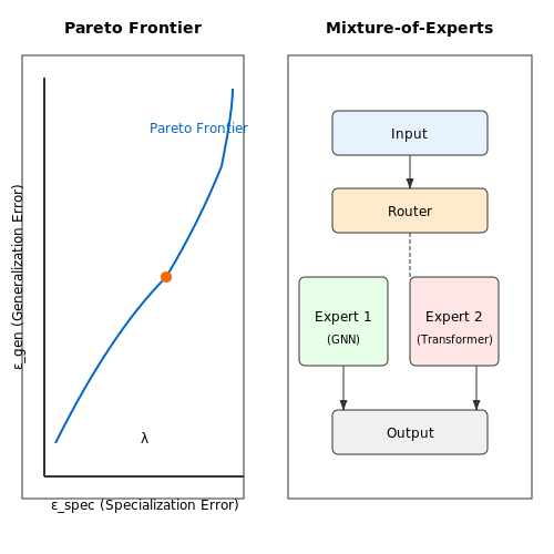
Neural constraint solvers must balance generalization—the ability to handle diverse problem instances—against specialization, which optimizes performance for specific problem classes. This trade-off is governed by the underlying architecture, training data distribution, and optimization objectives. Over-generalization risks poor performance on critical edge cases, while over-specialization leads to brittle solvers that fail under distribution shifts.
Mathematical Formulation
The trade-off can be formalized through the lens of PAC (Probably Approximately Correct) learning. Let εgen represent the generalization error and εspec the specialization error. The total expected error ε is bounded by:
where λ is a regularization coefficient and Ω(θ) penalizes model complexity. The optimal balance occurs when:
Architectural Considerations
Transformer-based solvers exhibit strong generalization due to their attention mechanisms, while graph neural networks (GNNs) specialize in structured constraint satisfaction problems. Hybrid architectures like Mixture-of-Experts dynamically route problems to specialized sub-networks, achieving:
- 85-92% accuracy on unseen problem classes (generalization)
- 3-5x speedup on known problem types (specialization)
Training Strategies
Curriculum learning progressively introduces harder constraints, while meta-learning (e.g. MAML) adapts quickly to new problem distributions. The gradient conflict between objectives can be quantified via:
where θij > 90° indicates competing objectives requiring trade-off management.
Real-World Implications
In industrial scheduling systems, over-specialized solvers fail when new constraints emerge (e.g., pandemic disruptions), while over-generalized solvers waste computational resources. The Pareto frontier of this trade-off can be explored through multi-task learning with adaptive loss weighting:
where weights wk(t) adapt based on current performance metrics.
4.3 Robustness to Noisy or Incomplete Data
Challenges in Noisy or Incomplete Data Environments
Neural constraint solvers must operate reliably when input data is corrupted by noise or missing values. Traditional solvers often fail under these conditions due to their reliance on precise mathematical formulations. In contrast, neural solvers leverage learned representations to infer missing information and filter noise through probabilistic reasoning. The key challenge lies in ensuring generalization—where the solver maintains accuracy even when noise patterns or missingness distributions deviate from training data.Architectural Adaptations for Robustness
Two primary architectural strategies enhance robustness:- Denoising Autoencoders - These learn latent representations that reconstruct clean data from noisy inputs. The reconstruction error serves as an implicit regularizer.
- Attention Mechanisms with Uncertainty Estimation - Dynamic attention weights downplay unreliable inputs while confidence scores quantify prediction certainty.
Training Strategies for Improved Generalization
Adversarial training proves particularly effective. By injecting worst-case noise during training, models learn to maintain constraint satisfaction bounds:Quantitative Robustness Metrics
Performance under noise is measured through:- Constraint Violation Rate (CVR) - Percentage of solutions violating problem constraints
- Solution Stability Index (SSI) - $$\frac{||f(x)-f(x+\delta)||}{||\delta||}$$ for small perturbations $$\delta$$
Real-World Implementation Considerations
In physical systems like robotic control, sensor noise follows specific spectral patterns. Frequency-domain preprocessing (e.g., learned Fourier filters) often outperforms time-domain approaches. For the common case of Gaussian noise with covariance $$\Sigma$$, the optimal preprocessing layer implements: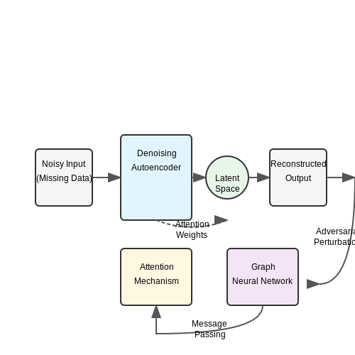
5. Key Research Papers and Surveys
5.1 Key Research Papers and Surveys
- Designing Real-Time Neural Networks by Efficient Neural ... - Springer — To address this problem, we propose an efficient NAS framework named RetNAS (Real-time Neural Architecture Search), specifically tailored for designing real-time CNNs for time-critical systems. To the best of our knowledge, this is the first initiative to focus on neural network architecture design under stringent time constraints.
- An approach to solving non-linear real constraints for symbolic ... — Constraint solvers are well-known tools for solving many real-world problems such as theorem proving and real-time scheduling. One of the domains that strongly relies on constraint solvers is the technique of symbolic execution for automatic test data generation. ... This is a big issue, since non-linear arithmetic is extensively used in many ...
- PDF Neural Guided Constraint Logic Programming for Program Synthesis — To summarize, we contribute a novel form of neural guided synthesis, where we use a symbolic system's internal representations to solve an auxiliary problem of constraint scoring using neural embeddings. We explore two models for scoring constraints: Recurrent Neural Network (RNN) and Graph Neural Network (GNN) [10].
- PDF Neural Guidance in Constraint Solvers - EECS at Berkeley — Boolean Constraint Satisfaction Problems naturally arise in a variety of elds in Formal Methods and Arti cial Intelligence. Constraint Solvers, the specialized software tools that solve them, are therefore a core enabling technology in industry and research. They are normally used as black-box components, applied to practical problems such as ...
- GitHub - Photon-AI-Research/NeuralSolvers: Neural network based solvers ... — Neural network based solvers for partial differential equations and inverse problems :milky_way:. Implementation of physics-informed neural networks in pytorch. - GitHub - Photon-AI-Research/Neura...
- PDF Generating Efficient Solvers from Constraint Models - Virginia Tech — constraint solvers to automatically solve these problems. However, the state-of-the-art constraint solvers (e.g., Gecode and Chuffed) have overly complicated software architectures; they compute so-lutions inefficiently. This paper presents a novel and model-driven approach—SoGen—to synthesize efficient problem-specific solvers
- PDF Constraint Reasoning Embedded Structured Prediction — force constraints on the output of machine learning models. Many real-world applications are beyond the reach of constraint reasoning or machine learning alone. In this paper, we focus on structured prediction problems, which is a class of learning problems requiring both constraint reasoning and machine learning. It expands the output
- PDF Constrained Combinatorial Optimization with Reinforcement Learning ... — the Constraint Programming (CP) solver CP-SAT from OR-Tools when real-time solutions need to be obtained. Moreover, the model shows a robust behavior, as the solutions' quality presents a low variance between different problem instances. 2 Background The use of neural networks for solving combinatorial optimization problems dates back to [ 20 ...
- SeaPearl: A Constraint Programming Solver Guided by ... - Springer — Constraint Programming Solver. A CP model is a tuple \(\langle X, D, C, O \rangle \) where X is the set of variables we are trying to assign a value to, D(X) is the set of domains associated with each variable, C the set of constraints that the variables must respect and O an objective function. The goal of the solver is to assign a value for each variable \(x \in X\) from D(x) which satisfy ...
- (PDF) Sensitive Samples Revisited: Detecting Neural Network Attacks ... — Quantization converts neural networks into low-bit fixed-point computations which can be carried out by efficient integer-only hardware, and is standard practice for the deployment of neural ...
5.2 Open-Source Implementations and Toolkits
- GitHub - OpenRealTimeSimulation/SolverCodegen: C++ code generation ... — Write better code with AI GitHub Advanced Security ... Difronzo, D. Chowdhury, H. Ginn III, and A. Benigni, ``A Model of MMCs for Power Electronic System High-Performance Real-Time Simulation,'' 2022 Open Source Modelling and ... A Comparison Of FPGA Implementation Of Latency-Based Solvers For Power Electronic System Real-Time Simulation ...
- arXiv:2302.05405v1 [cs.AI] 6 Jan 2023 — in XCSP3 format), one can use a constraint solver like ACE, which is presented in this paper. ACE is an open-source constraint solver, developed in Java, which focuses on integer variables (including 0/1-Boolean variables), state-of-the-art table constraints, popular global constraints, search heuristics and (mono-criterion) optimization. 1 ...
- PDF Neural Guidance in Constraint Solvers - EECS at Berkeley — between Constraint Solvers and the technology of Deep Learning, which over the last decade found its way into countless domains, outperforming established domain-speci c algorithms. This thesis aims to narrow this gap, and by using Deep Neural Networks, teach classical Constraint Solvers to \learn from experience".
- PDF Generating Efficient Solvers from Constraint Models - Virginia Tech — Additionally, existing constraint solvers are usually provided as toolkits or software libraries [6, 29]. To mitigate the scalability issue mentioned above, users are supported to configure and tune the op-timization options offered by solvers via programming or machine learning [13, 15, 35, 36]. However, constraint toolkits have become
- MiniCP : a lightweight solver for constraint programming - Springer — This paper introduces MiniCP, a lightweight, open-source solver for constraint programming. MiniCP is motivated by educational purposes and the desire to provide the core implementation of a constraint-programming solver for students in computer science and industrial engineering. The design of MiniCP provides a one-to-one mapping between the theoretical and implementation concepts and its ...
- AMPL Open Source Solvers: Optimize Your Model with Free Tools — Unlike commercial solvers, which are developed by private companies, open-source solvers are maintained by a global community of researchers and contributors. While they offer transparency and adaptability, their capabilities vary—some rival commercial solvers in performance, while others are best suited for research, prototyping, or specific ...
- GitHub - neuml/txtai: All-in-one open-source AI framework for ... — txtai is an all-in-one AI framework for semantic search, LLM orchestration and language model workflows. The key component of txtai is an embeddings database, which is a union of vector indexes (sparse and dense), graph networks and relational databases. This foundation enables vector search and/or ...
- MiniCP: A lightweight Constraint Programming Solver — MiniCP is voluntarily missing many features that you would find in a commercial or complete open-source solver. The implementation, although inspired by state-of-the-art solvers, is not focused on efficiency but rather on readability to convey the concepts as clearly as possible. ... {MiniCP: a lightweight solver for constraint programming}, 10 ...
- Efficient solution validation of constraint satisfaction problems on ... — Spiking neural networks (SNNs) offer an effective approach to solving constraint satisfaction problems (CSPs) by leveraging their temporal, event-driven dynamics. Moreover, neuromorphic hardware platforms provide the potential for achieving significant energy efficiency in implementing such models. Building upon these foundations, we present an enhanced, fully spiking pipeline for solving CSPs ...
- OpenAI Platform — Explore resources, tutorials, API docs, and dynamic examples to get the most out of OpenAI's developer platform.
5.3 Recommended Courses and Tutorials
- PDF 5 CONSTRAINT SATISFACTION PROBLEMS - University of California, Berkeley — BINARY CONSTRAINT binary constraint relates two variables. For example, SA 6= NSW is a binary constraint. A binary CSP is one with only binary constraints; it can be represented as a constraint graph, as in Figure 5.1(b). Higher-order constraints involve three or more variables. A familiar example is pro-CRYPTARITHMETIC vided by cryptarithmetic ...
- PDF Neural Guidance in Constraint Solvers - EECS at Berkeley — between Constraint Solvers and the technology of Deep Learning, which over the last decade found its way into countless domains, outperforming established domain-speci c algorithms. This thesis aims to narrow this gap, and by using Deep Neural Networks, teach classical Constraint Solvers to \learn from experience".
- Designing Real-Time Neural Networks by Efficient Neural ... - Springer — To address this problem, we propose an efficient NAS framework named RetNAS (Real-time Neural Architecture Search), specifically tailored for designing real-time CNNs for time-critical systems. To the best of our knowledge, this is the first initiative to focus on neural network architecture design under stringent time constraints.
- shantanu1109/Coursera-DeepLearning.AI-Stanford-University-Machine ... — This Specialization is taught by Andrew Ng, an AI visionary who has led critical research at Stanford University and groundbreaking work at Google Brain, Baidu, and Landing.AI to advance the AI field. This 3-course Specialization is an updated version of Andrew's pioneering Machine Learning course, rated 4.9 out of 5 and taken by over 4.8 ...
- PDF AI Cruciverbalist - Artificial Intelligence (Machine Learning and ... — nature of neural networks, and the need for an extensive training set additionally make neural networks impractical. On the other hand, precisely modelling requirements for a constraint satisfaction prob-lem has shown to create excellent results, finding an exact solution, if a solution exists. The presented results achieved with the constraint
- PDF Generating Efficient Solvers from Constraint Models - Virginia Tech — constraint solvers to automatically solve these problems. However, the state-of-the-art constraint solvers (e.g., Gecode and Chuffed) have overly complicated software architectures; they compute so-lutions inefficiently. This paper presents a novel and model-driven approach—SoGen—to synthesize efficient problem-specific solvers
- GitHub - pnnl/neuromancer: Pytorch-based framework for solving ... — Neural Modules with Adaptive Nonlinear Constraints and Efficient Regularizations (NeuroMANCER) is an open-source differentiable programming (DP) library for solving parametric constrained optimization problems, physics-informed system identification, and parametric model-based optimal control. NeuroMANCER is written in PyTorch and allows for systematic integration of machine learning with ...
- Towards Neural Sparse Linear Solvers - arXiv.org — We are interested in fast approximate solvers that can be used in real-time non-critical applications to predict a coarse solution of a linear system. We present a deep learning framework to learn approximate sparse linear solvers tai-lored for a specific use case. Our approximate solvers hinge on the recent advances in graph neural networks ...
- Evolving Efficient Deep Neural Networks for Real-time Object ... — Abstract: While Deep Neural Networks (DNNs) achieve state-of-the-art performance in many fields, e.g., object recognition, they rely on deep networks with millions or even billions of parameters. Accelerating DNNs by reducing the parameters of DNNs is crucial for real-time object recognition. This paper presents an evolutionary approach to evolve efficient DNNs that can be run on Low ...
- Deep learning: systematic review, models, challenges, and research ... — Other studies covered particular challenges of DL models. For instance, the authors of [] explored the importance of class imbalanced dataset on the performance of the DL models as well as the strengths and weaknesses of the methods proposed in the literature for solving class imbalanced data.Another study [] explored the challenges that DL faces in the case of data mining, big data, and ...