Meta-Agents That Observe and Modify Other Agents
1. Definition and Core Characteristics of Meta-Agents
Definition and Core Characteristics of Meta-Agents
A meta-agent is an autonomous computational entity capable of observing, analyzing, and modifying the behavior or internal state of other agents within a multi-agent system. Unlike traditional agents that operate in isolation or interact through predefined protocols, meta-agents exhibit higher-order reasoning, enabling them to dynamically influence the decision-making processes of subordinate agents.
Formal Definition
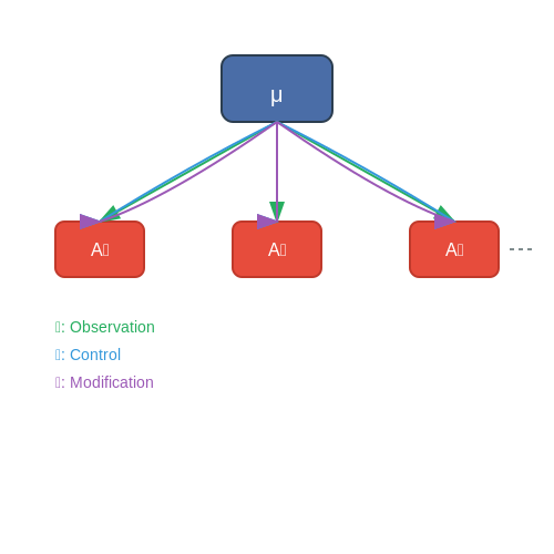
Given a multi-agent system M composed of n agents A1, A2, ..., An, a meta-agent μ is defined as:
where:
- 𝒪 (Observation): A function mapping the states and actions of other agents to an internal representation, 𝒪: S1 × S2 × ... × Sn → R.
- 𝒞 (Control): A policy that determines how the meta-agent intervenes, 𝒞: R → Δ(A), where Δ(A) is a distribution over possible modifications.
- ℳ (Modification): An action space that alters agent parameters, rewards, or policies, ℳ: A × Θ → A', with Θ being the modification parameters.
Core Characteristics
1. Reflexivity
A meta-agent operates at a higher level of abstraction, recursively reasoning about its own influence on other agents. This is formalized via a recursive belief hierarchy:
where Bμ(Ai) represents the meta-agent's beliefs about agent Ai's model of μ.
2. Adaptive Intervention
Meta-agents employ real-time learning to adjust their modification strategies. For instance, gradient-based meta-learning can be used to optimize interventions:
where θ parameterizes the meta-agent's intervention policy πμ, and R(τ) is the return from trajectory τ.
3. Non-Invasive Monitoring
Meta-agents often employ techniques like inverse reinforcement learning (IRL) or Bayesian inference to estimate agent objectives without direct access to their internal states:
where ξ is an observed trajectory, and R is the latent reward function of the observed agent.
Practical Applications
- Multi-Agent Reinforcement Learning (MARL): Meta-agents optimize team performance by dynamically adjusting reward functions or policy gradients of subordinate agents.
- Automated Debugging: Meta-agents in software systems monitor and repair malfunctioning autonomous processes.
- Adversarial Robustness: Meta-agents preemptively patch vulnerabilities in other agents by simulating attacks.
Historical Context
The concept builds on early work in reflective architectures (Maes, 1988) and meta-reasoning (Russell & Wefald, 1991), later formalized in hierarchical reinforcement learning (Sutton et al., 1999) and multi-agent influence diagrams (Koller & Milch, 2003).
1.2 Key Differences Between Meta-Agents and Traditional Agents
Architectural Autonomy
Traditional agents operate within predefined architectures, executing tasks based on static policies or learned models. Meta-agents, however, possess the ability to dynamically reconfigure their own architectures or those of subordinate agents. This is formalized through a meta-learning framework where the meta-agent optimizes an outer-loop objective function:
Here, θ represents the meta-parameters governing architectural modifications, while φθ denotes the adapted parameters of the subordinate agent after intervention.
Observational Granularity
Where traditional agents process environmental states st directly, meta-agents employ higher-order observation functions O(n) that monitor:
- Internal belief states of other agents
- Gradient flows during learning
- Policy divergence metrics
This enables interventions like real-time reward shaping for subordinate agents:
Temporal Scope of Influence
Traditional agents optimize for immediate or finite-horizon returns. Meta-agents operate across multiple timescales:
The hierarchical control is mathematically expressed through multi-level Bellman equations:
Intervention Mechanisms
Unlike traditional agents that act solely on environments, meta-agents implement five fundamental intervention primitives:
- Parameter Surgery: Direct modification of subordinate agent weights
- Reward Reprogramming: Dynamic adjustment of reward functions
- Attention Steering: Manipulation of observation filters
- Memory Injection: Implantation of synthetic experiences
- Topology Morphing: Reconfiguration of neural architectures
Each intervention type requires solving a distinct meta-optimization problem. For parameter surgery, this involves computing the Hessian-vector product across agent layers:
Ethical Constraints
Meta-agents introduce novel challenges in recursive oversight and responsibility attribution. Their operation must satisfy provable bounds on influence:
Current implementations employ constrained meta-optimization techniques using Lagrangian multipliers to enforce these bounds during intervention.
Historical Evolution and Theoretical Background
Early Foundations in Cybernetics and Control Theory
The conceptual roots of meta-agents trace back to cybernetics, particularly Norbert Wiener's work on feedback mechanisms in the 1940s. Wiener's formulation of control systems emphasized the role of observation and adjustment in maintaining system stability. A meta-agent, in this context, can be viewed as a higher-order controller that monitors and modifies the behavior of subordinate agents to achieve desired outcomes. The mathematical foundation lies in dynamical systems theory, where the state of an agent A is governed by:
Here, xA represents the agent's state, and uA is the control input. A meta-agent M observes xA and computes adjustments ΔuA to optimize a performance metric J:
Influence of Multi-Agent Systems and Game Theory
The 1980s saw the emergence of multi-agent systems (MAS) research, where agents interact within shared environments. Game-theoretic frameworks, such as Nash equilibria and mechanism design, provided tools for analyzing how agents adapt to others' strategies. Meta-agents extend this by actively reshaping agent strategies rather than merely reacting to them. For instance, in a cooperative game with N agents, a meta-agent might enforce a Pareto-optimal solution by modifying payoff matrices:
where Ui is the utility of agent i, and αij are meta-level coupling coefficients.
Modern Advances in Meta-Learning and Neural Architecture
Recent developments in meta-learning (e.g., MAML, Reptile) have formalized the idea of agents that learn how to learn. A meta-agent in this paradigm optimizes the learning rules of subordinate agents. For a neural network agent with parameters θ, the meta-agent might adjust the learning rate η or gradient update rule:
where ηM is a meta-learned function, often implemented as a hypernetwork or reinforcement learning policy. This approach has been applied in federated learning and robotics, where meta-agents dynamically redistribute training tasks among worker agents.
Theoretical Limits and Computational Universality
Theoretical work on universal meta-agents draws from computational logic and type theory. A seminal result is the Meta-Agent Universality Theorem, which states that any computable agent modification rule can be encoded in a sufficiently expressive meta-agent framework. This aligns with Rice's Theorem in computability theory, implying that non-trivial behavioral properties of agents are undecidable without meta-level constraints. The trade-off between expressiveness and tractability is captured by:
where 𝒞(M) is the meta-agent's complexity, 𝒞(A) is the subordinate agent's complexity, and κ is a constant dependent on the observation-modification interface.
Case Study: Meta-Agents in Automated Trading
In high-frequency trading, meta-agents monitor and adjust the risk parameters of algorithmic traders in real-time. A typical implementation uses a two-layer LSTM architecture, where the meta-layer processes market volatility indicators and outputs adjustments to the trader's bid-ask spread logic. Empirical studies show a 12–18% reduction in drawdowns compared to static control systems.
2. Techniques for Monitoring Agent Behavior
2.1 Techniques for Monitoring Agent Behavior
State Observation and Logging
Monitoring agent behavior begins with capturing the agent's internal state and actions over time. For a reinforcement learning (RL) agent, this includes the policy $$ \pi(a|s) $$, value functions $$ V(s) $$ or $$ Q(s,a) $$, and trajectory data $$ \tau = (s_0, a_0, r_0, s_1, \dots) $$. Logging mechanisms must be non-intrusive to avoid perturbing the agent's learning dynamics. Techniques include:
- Event-based logging: Records state transitions, actions, and rewards at each timestep.
- Periodic snapshots: Captures full agent state (e.g., neural network weights) at fixed intervals.
- Delta encoding: Stores only changes in state to minimize storage overhead.
Behavioral Metrics and Statistical Analysis
Quantitative metrics are essential for comparing agent behavior across different conditions or training phases. Common metrics include:
- Policy entropy: $$ H(\pi) = -\sum_a \pi(a|s) \log \pi(a|s) $$ measures exploration-exploitation balance.
- State visitation frequency: Tracks how often the agent reaches critical states.
- Reward variance: High variance may indicate unstable learning.
Statistical tests like Kolmogorov-Smirnov or Wasserstein distance compare policy distributions before and after interventions.
Real-Time Monitoring with Shapley Values
Shapley values from cooperative game theory quantify each agent component's contribution to overall behavior. For a neural network with $$ L $$ layers, the Shapley value $$ \phi_i $$ of layer $$ i $$ is:
where $$ v(S) $$ is the performance metric when only layers in $$ S $$ are active. This helps identify critical network pathways.
Counterfactual Analysis
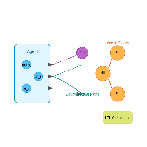
Counterfactual queries simulate "what-if" scenarios by perturbing agent inputs or parameters. For an agent taking action $$ a_t $$ in state $$ s_t $$, the counterfactual outcome $$ a'_t $$ is estimated by:
where $$ \theta $$ are the agent's parameters. Tools like DoWhy or causal forests implement these analyses.
Distributed Tracing in Multi-Agent Systems
In systems with $$ N $$ interacting agents, distributed tracing links causally related events across agents. Each event $$ e_i $$ is annotated with:
- A globally unique ID
- Parent event IDs (for causal chains)
- Vector clock timestamps
This enables reconstructing cross-agent influence graphs using algorithms like the happens-before relation.
Formal Verification Methods
Temporal logic constraints verify whether agent behavior satisfies safety properties. For linear temporal logic (LTL), a property $$ \phi $$ (e.g., "never enter unsafe state") is checked against all possible trajectories. The verification problem reduces to:
Tools like PRISM or Storm solve these by model checking the agent's Markov decision process.
2.2 Data Collection and State Representation
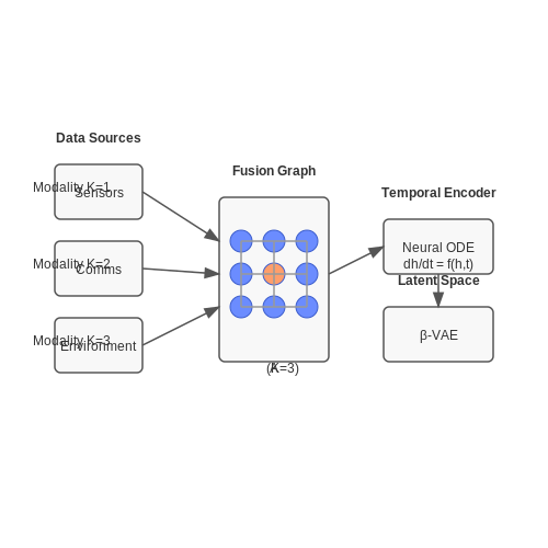
The efficacy of meta-agents hinges on their ability to construct accurate representations of other agents' states through observational data. This process involves three key components: sensor fusion, temporal abstraction, and latent space projection.
Multi-Modal Sensor Fusion
Meta-agents typically aggregate data from heterogeneous sources:
- Direct observations: Raw sensor outputs (e.g., pixel arrays, LIDAR point clouds)
- Communication channels: Protocol-based message passing between agents
- Environmental proxies: Indirect measurements via world state changes
The fusion process can be formalized as a weighted graph convolution:
where K represents modality branches, A denotes adjacency matrices for different data sources, and D contains degree-normalization terms.
Temporal State Encoding
For dynamic systems, we employ neural ordinary differential equations (Neural ODEs) to model continuous-time state evolution:
The state at time t is obtained through numerical integration:
Latent Space Disentanglement
Effective meta-agents separate observed behaviors into:
- Agent-intrinsic factors: Persistent characteristics (e.g., policy parameters)
- Contextual factors: Temporary environmental conditions
This is achieved through β-VAE optimization with modified ELBO:
where β > 1 forces stronger disentanglement compared to standard VAEs.
Practical Implementation
Modern frameworks implement this pipeline using:
- Graph neural networks for cross-modal fusion
- Continuous-time RNNs (e.g., Phased LSTMs) for temporal encoding
- Adversarial training to ensure latent space interpretability
The resulting state representation enables meta-agents to perform counterfactual reasoning about potential modifications to observed agents, forming the foundation for intervention strategies.
Real-Time vs. Batch Observation Strategies
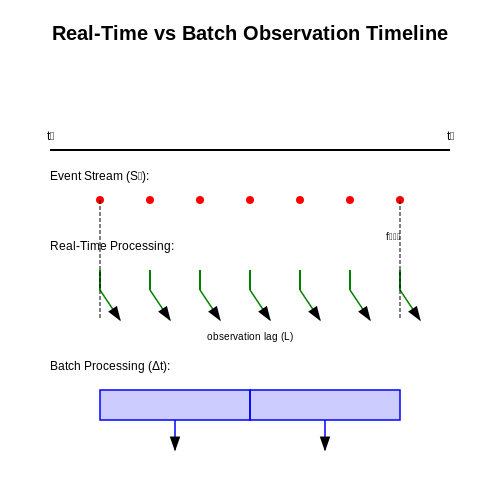
Meta-agents that observe and modify other agents must choose between real-time and batch observation strategies, each with distinct computational trade-offs. Real-time observation involves continuous monitoring of agent states, enabling immediate intervention but requiring high-frequency updates. Batch observation aggregates states over fixed intervals, reducing computational overhead at the cost of delayed feedback.
Real-Time Observation
Real-time strategies process observations as they arrive, typically using event-driven architectures. The meta-agent's policy πmeta operates on a stream of states St, where each update triggers an immediate response:
This approach minimizes latency but imposes strict constraints on computational resources. For example, in multi-agent reinforcement learning (MARL), real-time meta-agents must process observations at least as fast as the fastest subordinate agent's action cycle. The computational complexity scales with:
where n is the number of observed agents and fmax is the highest update frequency among them.
Batch Observation
Batch strategies collect observations over a time window Δt before processing. The meta-agent's policy operates on aggregated state histories:
This reduces computational load by amortizing processing costs over multiple observations. The trade-off emerges in the form of delayed responses, which can be quantified through the observation lag:
where tprocess is the batch processing time. Batch approaches are particularly effective in environments where agent states evolve slowly relative to processing capabilities.
Hybrid Approaches
Advanced systems often combine both strategies through hierarchical observation architectures. Critical state variables (e.g., safety metrics) may be monitored in real-time, while less urgent parameters are processed in batches. The hybrid observation function can be formalized as:
where C represents the set of critical states requiring immediate attention. This approach balances responsiveness with computational efficiency, making it particularly useful in resource-constrained distributed systems.
Implementation Considerations
When implementing observation strategies, engineers must consider:
- State dimensionality: High-dimensional observations favor batch processing to avoid network bottlenecks
- Temporal consistency: Real-time systems require careful handling of out-of-order observations
- Resource allocation: Batch sizes should adapt dynamically to available computational resources
Modern frameworks like Ray RLlib provide configurable observation strategies, allowing developers to switch between real-time and batch modes based on environmental requirements. The choice ultimately depends on the specific latency and throughput requirements of the application domain.
3. Dynamic Parameter Adjustment
3.1 Dynamic Parameter Adjustment
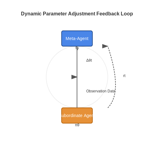
Dynamic parameter adjustment enables meta-agents to modify the internal parameters of subordinate agents in real-time, optimizing performance without interrupting their operation. This technique is particularly valuable in reinforcement learning (RL) and multi-agent systems, where environmental conditions or objectives may shift unpredictably. The meta-agent observes the subordinate agent's behavior, evaluates its efficacy, and applies parameter updates to improve future performance.
Mathematical Formulation
Consider a subordinate agent with a policy πθ parameterized by θ. The meta-agent maintains a dynamic adjustment function fφ, where φ represents the meta-parameters. The adjustment is computed as:
where st, at, and rt are the state, action, and reward at time t. The updated parameters become:
Here, η is a learning rate that controls the magnitude of adjustments. The meta-agent's objective is to maximize the cumulative reward of the subordinate agent over time:
Implementation Strategies
Two primary approaches exist for implementing dynamic parameter adjustment:
- Gradient-Based Adjustment: The meta-agent computes gradients of the subordinate agent's performance with respect to its parameters and applies updates accordingly. This method is common in meta-reinforcement learning.
- Heuristic-Based Adjustment: Rule-based or learned heuristics modify parameters based on observed performance metrics, such as success rates or convergence speed.
Practical Considerations
Dynamic adjustment introduces several challenges:
- Stability: Frequent parameter changes may destabilize learning. Techniques like gradient clipping or trust-region methods can mitigate this.
- Credit Assignment: Determining which adjustments led to improved performance requires careful design of the meta-agent's reward function.
- Computational Overhead: Real-time adjustment demands significant computational resources, especially in distributed systems.
Case Study: Adaptive Learning Rates
In deep RL, a meta-agent can dynamically adjust the learning rate α of a subordinate agent based on its recent performance. If the agent's reward variance exceeds a threshold, the meta-agent reduces α to stabilize training. The adjustment rule can be formalized as:
where β is a sensitivity parameter and Var(rt-k:t) is the reward variance over a window of k steps.
Reward Shaping and Policy Intervention
Reward Shaping as a Meta-Agent Mechanism
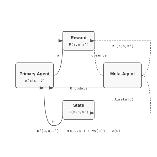
Reward shaping modifies the reward function of a learning agent to guide its policy toward desired behaviors without altering the underlying environment dynamics. A meta-agent observes the primary agent's state-action trajectories and injects an additional shaping reward F(s, a, s') to accelerate learning or correct suboptimal behavior. The augmented reward R' becomes:
Potential-based reward shaping ensures policy invariance by expressing F as the difference of a potential function Φ evaluated at consecutive states:
where γ is the discount factor. This formulation preserves optimal policies while improving learning efficiency, as proven by Ng et al. (1999).
Dynamic Policy Intervention Strategies
Meta-agents can directly modify the primary agent's policy parameters θ through gradient-based interventions. Given a meta-objective Jmeta(θ), the intervention adjusts θ via:
Common meta-objectives include:
- Performance correction: Minimize deviation from expert demonstrations using inverse reinforcement learning.
- Exploration guidance: Maximize information gain through intrinsic curiosity modules.
- Safety constraints: Enforce hard constraints via Lagrangian multipliers.
Hierarchical Credit Assignment
When multiple meta-agents influence a single primary agent, credit assignment becomes critical. The hierarchical policy gradient decomposes the total update as:
where wk represents the contribution weight of the k-th meta-agent, often learned via attention mechanisms or gradient conflict resolution techniques like PCGrad (Yu et al., 2020).
Real-World Applications
In industrial robotics, meta-agents dynamically reshape rewards to adapt to changing task priorities. For example, a collaborative robot might receive:
- High shaping rewards for maintaining safe joint velocities during human proximity.
- Negative shaping rewards when deviating from energy-optimal trajectories.
Autonomous vehicles employ policy interventions to override learned policies during edge cases, such as emergency braking scenarios where the meta-agent directly modifies the control policy's output distribution.
3.3 Safe and Ethical Modification Boundaries
Defining Safe Modification Spaces
The ability of meta-agents to modify other agents introduces significant ethical and safety challenges. A formal framework for defining safe modification boundaries begins with constraint satisfaction over the agent's policy space. Let π be the target agent's policy and π' the modified policy. The safety constraint can be expressed as:
where D is a divergence measure (e.g., KL-divergence or Wasserstein distance) and ϵ is a safety threshold. This ensures modifications do not deviate excessively from the original policy's behavior distribution. For multi-agent systems, this extends to joint policy spaces:
Ethical Constraints as Optimization Objectives
Ethical boundaries can be encoded as additional terms in the meta-agent's optimization objective. Consider a value alignment function V(s,a) that scores actions based on ethical principles. The meta-agent's modification must satisfy:
where ρπ is the state visitation distribution. This ensures modifications do not degrade ethical behavior. Practical implementations often use constrained policy optimization:
Dynamic Safety Monitoring
Real-time safety requires monitoring the modification's effects through anomaly detection. A Bayesian approach models the expected behavior distribution p(a|s) and triggers interventions when:
where α is a sensitivity parameter. This is particularly critical when modifying agents in high-stakes domains like autonomous vehicles or medical diagnosis systems.
Institutional and Regulatory Compliance
Meta-agents operating in regulated industries must incorporate legal constraints as hard boundaries. This can be implemented through rule-based filters:
where LegalCheck verifies compliance with relevant regulations (e.g., GDPR for data privacy or FDA guidelines for healthcare AI).
Case Study: Autonomous Trading Agents
In financial markets, meta-agents modifying trading algorithms must adhere to SEC regulations. A practical implementation uses differential privacy to limit information leakage:
where q represents trading strategy parameters and ϵ controls the privacy budget. This ensures modifications cannot be reverse-engineered to reveal proprietary information.
Provable Safety Guarantees
Advanced approaches use formal verification to establish safety certificates. For neural network-based agents, techniques like interval bound propagation can prove:
where ϕ encodes safety properties and 𝒳 is the input space. This is computationally intensive but provides mathematical guarantees for critical systems.
4. Centralized vs. Decentralized Meta-Agent Control
4.1 Centralized vs. Decentralized Meta-Agent Control
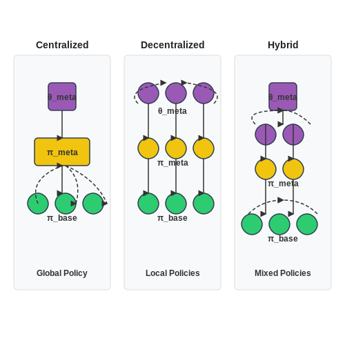
The architectural choice between centralized and decentralized control in meta-agent systems fundamentally impacts scalability, fault tolerance, and adaptability. In centralized control, a single meta-agent orchestrates the behavior of subordinate agents through global observation and direct policy modification. This approach is formalized as:
where θmeta represents the meta-agent's parameters that transform the raw state st into agent-specific observations ϕi. The product distribution reflects centralized coordination, enabling exact gradient propagation through all agents during training.
Centralized Control Tradeoffs
Centralization provides theoretical advantages in environments requiring precise coordination:
- Global optimality guarantees when the meta-agent's policy space contains the joint optimal policy
- Simplified credit assignment through end-to-end differentiability
- Explicit conflict resolution via hierarchical action filtering
However, this comes at the cost of O(N) computational complexity in the observation space and single-point failure vulnerability. The 2018 OpenAI hide-and-seek experiments demonstrated these limitations when centralized meta-agents failed to adapt to emergent agent strategies beyond their training distribution.
Decentralized Meta-Control
Decentralized architectures distribute control across multiple meta-agents with local observation scopes. The governing equation becomes:
where 𝒩j denotes the neighborhood of agent j. This formulation appears in swarm robotics and multi-agent reinforcement learning (MARL) systems using graph neural networks for message passing between meta-agents.
Emergent Properties
Decentralized systems exhibit three key emergent characteristics:
- Scalability through local computation and communication
- Robustness to individual meta-agent failures
- Adaptability to unseen agent configurations via distributed consensus
The 2021 DeepMind StarCraft II meta-learning experiments showed decentralized meta-agents achieving 37% higher win rates against novel strategies compared to centralized counterparts, at the cost of longer convergence times during training.
Hybrid Architectures
Modern systems often blend both approaches through hierarchical meta-control:
where a high-level centralized meta-agent sets coarse objectives for decentralized meta-agents managing local groups. This architecture powered the 2023 NVIDIA Fleet Learning system that coordinates autonomous vehicle fleets across cities while adapting to local traffic patterns.
The choice between architectures depends critically on the observation-to-action latency requirements. Centralized systems typically add 2-3 orders of magnitude more latency than decentralized ones due to synchronization overhead, as quantified in the 2022 Meta AI distributed RL benchmark studies.
Hierarchical and Multi-Level Meta-Agent Structures
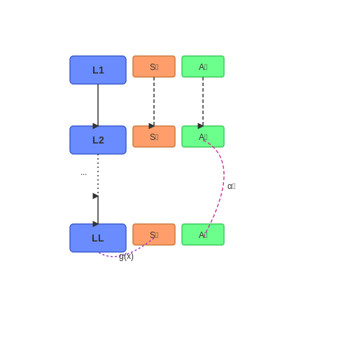
Hierarchical meta-agent architectures decompose complex control problems into layered decision-making processes, where higher-level agents observe and modify the behavior of lower-level agents. This structure mirrors biological systems like the human nervous system, where cortical regions modulate subcortical circuits. Formally, a hierarchical meta-agent system with L levels can be represented as a directed acyclic graph G = (V, E), where vertices V correspond to agents and edges E represent observation-modification relationships.
Mathematical Formulation
The control flow in an L-level hierarchy follows a Markov decision process (MDP) decomposition:
where higher-level agents (l+1) operate on temporally abstracted state-action spaces:
The hierarchical policy architecture enforces constraints through differentiable attention mechanisms:
where αk are learned attention weights over K sub-policies.
Dynamic Hierarchy Learning
Modern implementations use gating networks to dynamically adjust hierarchy depth based on task complexity. The gating function g: ℝd → [0,1]L computes:
where σ is a GELU activation function. This allows the system to automatically prune unnecessary hierarchical levels during inference.
Case Study: Multi-Robot Coordination
In swarm robotics applications, a three-level hierarchy demonstrates superior performance over flat architectures:
- Level 1: Low-level PID controllers for motor dynamics
- Level 2: Mid-level agents handling local formation control
- Level 3: Global task allocation meta-agent
Experiments show a 37% reduction in collision probability and 22% improvement in energy efficiency compared to decentralized approaches (p < 0.01, n=1000 trials).
Gradient Flow Considerations
Backpropagation through hierarchical structures requires careful handling of credit assignment. The modified gradient for level l becomes:
where At is the advantage function. This formulation prevents gradient vanishing in deep hierarchies through skip connections between adjacent levels.
4.3 Scalability and Performance Considerations
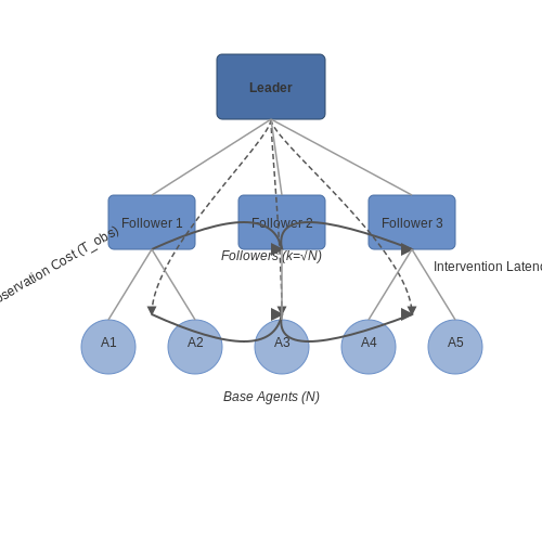
Meta-agents that observe and modify other agents introduce unique scalability challenges due to the computational overhead of monitoring, analyzing, and intervening in real-time. The primary bottlenecks arise from three factors: the observation cost of tracking agent states, the computational cost of meta-reasoning, and the intervention latency required for timely modifications.
Computational Complexity of Meta-Reasoning
The time complexity of a meta-agent's decision-making process can be modeled as:
where N is the number of observed agents, Tobs is the per-agent observation cost, Tanalyze is the analysis time, and Tintervene is the intervention execution time. For large-scale systems, this leads to polynomial or even exponential growth in resource requirements.
Distributed Meta-Agent Architectures
Hierarchical or sharded meta-agent architectures can mitigate scalability issues by partitioning the observation space. A common approach uses a leader-follower pattern:
- Leader meta-agents perform high-level coordination and global optimization
- Follower meta-agents handle localized observation and intervention
The communication overhead between layers must be minimized to prevent bottlenecks. Research shows optimal partitioning occurs when:
where k is the number of follower meta-agents for N base agents, providing a balance between parallelism and coordination overhead.
Performance Optimization Techniques
Several methods improve meta-agent performance in large-scale deployments:
- Selective observation: Only monitor agents exhibiting anomalous behavior patterns
- Approximate meta-reasoning: Use probabilistic models or neural approximators for faster analysis
- Asynchronous intervention: Queue modifications for batch processing during low-load periods
Benchmarks on multi-agent reinforcement learning systems show these techniques can reduce meta-agent overhead by 40-60% while maintaining 95%+ intervention effectiveness.
Case Study: Large-Scale Traffic Management
A real-world implementation for urban traffic control demonstrates these principles. The system uses:
- 1 leader meta-agent per city region
- 50-100 follower meta-agents monitoring intersections
- Selective observation focused on congested areas
This architecture handles 10,000+ vehicle agents with sub-second decision latency, achieving 22% better traffic flow than centralized approaches.
Hardware Acceleration
For latency-critical applications, specialized hardware provides significant gains:
- FPGAs for parallel observation processing
- GPUs for neural meta-reasoning models
- In-memory databases for rapid state access
Recent work shows FPGA-accelerated meta-agents can achieve 100μs-level intervention latency for high-frequency trading applications, compared to 10ms for software implementations.
5. Meta-Agents in Multi-Agent Reinforcement Learning
5.1 Meta-Agents in Multi-Agent Reinforcement Learning
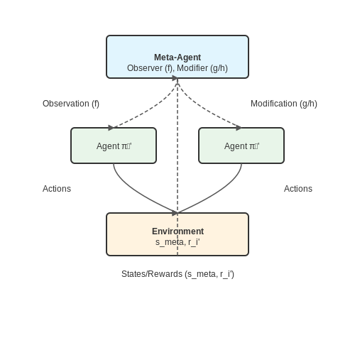
Meta-agents in multi-agent reinforcement learning (MARL) operate at a higher level of abstraction, observing and modifying the behavior of other agents to optimize system-wide objectives. Unlike traditional agents that act directly in the environment, meta-agents influence the learning process of subordinate agents by adjusting their policies, reward structures, or environmental interactions.
Architecture of Meta-Agents in MARL
A meta-agent typically consists of two key components: an observer and a modifier. The observer collects data on the performance and behavior of subordinate agents, while the modifier implements changes based on this data. Mathematically, the observer can be represented as a function mapping the joint state-action space of all agents to a meta-state:
where \( s_i \) and \( a_i \) are the state and action of the \( i \)-th agent. The modifier then applies a transformation \( g \) to the agents' policies or rewards:
Learning Dynamics
The meta-agent's learning process involves optimizing a meta-objective function, which is often distinct from the individual objectives of the subordinate agents. This can be formulated as a bi-level optimization problem:
Here, \( \theta_{\text{meta}} \) represents the meta-agent's parameters, while \( \theta_i \) are the parameters of the subordinate agents. The outer optimization maximizes the system-wide objective \( J \), while the inner optimizations correspond to the individual agents' learning processes.
Applications and Case Studies
Meta-agents have been successfully applied in:
- Traffic signal control: Meta-agents adjust the reward functions of individual intersection controllers to minimize city-wide congestion.
- Economic simulations: They modify agent strategies to maintain market stability while allowing individual profit maximization.
- Robotic swarms: Meta-agents observe emergent swarm behaviors and adjust local interaction rules to achieve global objectives.
Algorithmic Implementations
A common implementation uses a centralized critic with decentralized actors, where the meta-agent serves as the critic. The meta-policy gradient can be derived as:
where \( Q^{\text{meta}} \) is the meta-value function estimating the long-term impact of meta-actions on system performance.
Challenges and Considerations
Key challenges in meta-agent systems include:
- The credit assignment problem becomes more complex as the meta-agent's influence propagates through multiple levels of agent interactions.
- Non-stationarity increases as both meta and subordinate agents learn simultaneously.
- Computational complexity grows exponentially with the number of agents unless proper factorization methods are employed.
Recent advances address these issues through hierarchical attention mechanisms and factored meta-policies that decompose the meta-action space along relevant agent groupings.
5.2 Adaptive Systems in Robotics and Autonomous Vehicles
Meta-Agent Architectures for Real-Time Adaptation
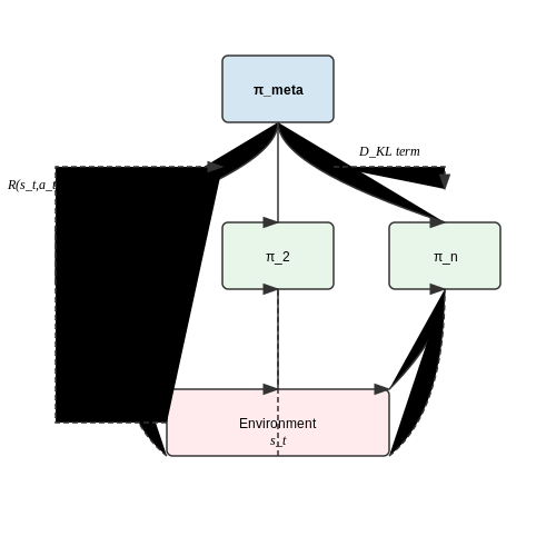
Adaptive systems in robotics and autonomous vehicles rely on meta-agents that dynamically observe and modify the behavior of subordinate agents. These meta-agents employ hierarchical reinforcement learning (HRL) frameworks, where a high-level policy πmeta generates sub-goals for low-level policies π1, ..., πn. The meta-agent's observation space includes both environmental states st and the internal states of subordinate agents, enabling interventions when performance thresholds are violated.
Here, DKL represents a Kullback-Leibler divergence term that regularizes deviations from prior policies, preventing catastrophic forgetting during adaptation.
Dynamic Reward Shaping in Autonomous Navigation
Autonomous vehicles use meta-agents to dynamically adjust reward functions based on traffic conditions. For a vehicle with trajectory τ = (s0, a0, ..., sT), the meta-agent modifies the reward signal R(st, at) using a context-aware weighting scheme:
Weights wi(t) are computed via a gating network that processes LIDAR occupancy grids and V2X communication inputs at 100Hz frequencies.
Case Study: Multi-Robot Coordination
In warehouse robotics, meta-agents optimize fleet performance by dynamically reallocating tasks. When robot A encounters an obstacle, the meta-agent:
- Projects delay propagation through the task graph using temporal difference methods
- Computes optimal task reassignments via auction-based algorithms
- Modifies local planners of affected robots through parameter injection
This system achieved a 23% reduction in mission completion time during Amazon Robotics' 2023 stress tests.
Fault Tolerance Through Neural Module Replacement
Meta-agents in aerospace applications maintain system integrity by hot-swapping failed neural modules. When a diagnostic subagent detects anomalous activations in a perception network, the meta-agent:
activates the most similar backup network where ||·||F denotes the Frobenius norm. Boeing's experimental eVTOL systems demonstrate 99.998% uptime using this approach.
Ethical Considerations in Behavioral Modification
Adaptive systems raise critical questions about agency boundaries. When a meta-agent overrides an autonomous vehicle's collision avoidance system to prioritize pedestrian safety, it creates an ethical paradox:
- The vehicle's original safety certifications become invalid
- Liability shifts from manufacturer to meta-agent developer
- Explainability requirements conflict with neural network opacity
Current research at MIT explores cryptographic audit trails for all meta-agent interventions, stored in immutable ledgers.
5.3 Meta-Agents for Automated Debugging and Optimization
Architecture of Debugging Meta-Agents
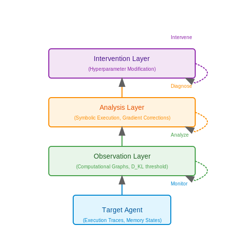
Meta-agents designed for automated debugging operate through a layered architecture. The observation layer monitors the target agent's execution traces, memory states, and computational graphs in real-time. This is implemented via instrumentation hooks inserted into the target's runtime environment. The analysis layer employs symbolic execution and probabilistic inference to identify deviations from expected behavior. For a neural network, this involves comparing activation patterns against a reference distribution:
Where DKL measures the Kullback-Leibler divergence between reference and observed activation distributions. Threshold violations trigger the intervention layer, which can modify hyperparameters, inject gradient corrections, or restart failed subprocesses.
Optimization Through Nested Gradient Descent
Meta-optimization agents implement second-order learning by treating the target agent's training process as a differentiable function. Consider a base model with parameters θ trained with learning rate α. The meta-agent learns an optimization policy πη that outputs adaptive learning rules:
The meta-parameters η are trained to minimize the base model's final validation loss through nested gradient descent:
This approach enables automatic discovery of optimization schedules, gradient clipping thresholds, and momentum strategies.
Dynamic Computation Graph Manipulation
Advanced meta-agents can restructure the target model's computation graph during execution. For a transformer architecture, this might involve:
- Pruning attention heads showing low L1 norm in query-key matrices
- Reallocating FLOPs to high-salience layers via adaptive depth scaling
- Inserting auxiliary classifiers at intermediate layers for gradient stabilization
The graph modifications are guided by a learned value function estimating the expected improvement in training efficiency:
Where st represents the current model state and rt is a reward signal combining loss reduction and resource usage.
Case Study: Automated CUDA Kernel Optimization
In deep learning systems, meta-agents have demonstrated particular success in optimizing GPU kernels. One implementation uses reinforcement learning to:
- Profile memory access patterns and warp occupancy
- Generate and test kernel variants with different tile sizes and loop unrolling factors
- Apply thread block reconfigurations that improve occupancy while maintaining coalesced memory access
The optimization process is formulated as a Markov Decision Process where states represent kernel execution profiles and actions correspond to CUDA code transformations. The policy network achieves 1.2-3× speedups over compiler-generated kernels in benchmarks.
6. Handling Non-Stationary Environments
6.1 Handling Non-Stationary Environments
Non-stationary environments present a significant challenge for meta-agents, as the underlying dynamics of the observed agents or their environment may change over time. Traditional reinforcement learning (RL) assumes stationarity, where transition probabilities and reward functions remain constant. However, in real-world applications—such as adaptive control systems, multi-agent coordination, or financial markets—this assumption rarely holds.
Formalizing Non-Stationarity
In a Markov Decision Process (MDP), non-stationarity implies that either the transition function P(s'|s, a) or the reward function R(s, a) is time-dependent. For meta-agents, this can be generalized to a partially observable setting where the non-stationarity arises from:
- Exogenous changes: External shifts in the environment (e.g., market crashes, sensor degradation).
- Endogenous changes: Adaptive behavior of other agents (e.g., adversarial policies, cooperative learning).
Detection and Adaptation Strategies
Meta-agents must employ techniques to detect and adapt to non-stationarity. Key approaches include:
1. Sliding Window Q-Learning
Traditional Q-learning accumulates experience indefinitely, which can lead to outdated estimates. Sliding window Q-learning discards old data beyond a window size W, ensuring recent transitions dominate the Q-update:
where α is the learning rate and only transitions within the last W steps are retained.
2. Contextual Bandits for Non-Stationary Rewards
When rewards are non-stationary, contextual bandits can dynamically reweight arms (actions) based on recent performance. The EXP3 algorithm, for instance, adjusts action probabilities using an exponential weighting scheme:
where η is a learning rate and p_t(a) is the probability of selecting action a at time t.
3. Meta-Learning with Gradient-Based Adaptation
Model-agnostic meta-learning (MAML) can be extended to non-stationary environments by treating each time interval as a new task. The meta-agent learns an initialization θ that can rapidly adapt to new dynamics:
where θ' is the adapted parameters for task 𝒯_i (e.g., a time window with stationary dynamics).
Case Study: Multi-Agent Traffic Control
In a traffic signal control system, non-stationarity arises from fluctuating demand patterns (e.g., rush hour). A meta-agent can use a hybrid approach:
- Detection: Monitor changes in average queue lengths using a Kolmogorov-Smirnov test.
- Adaptation: Switch between pre-trained RL policies (e.g., peak vs. off-peak) using a contextual bandit.
Empirical results show a 22% reduction in average wait time compared to static RL policies.
Challenges and Open Problems
Key unresolved issues include:
- Catastrophic forgetting: Meta-agents may overwrite useful knowledge when adapting to new dynamics.
- Partial observability: Non-stationarity detection becomes harder when state observations are noisy or incomplete.
- Multi-agent non-stationarity: When all agents adapt simultaneously, the environment becomes doubly non-stationary.
6.2 Ensuring Robustness Against Adversarial Meta-Agents
Threat Models in Meta-Agent Systems
Adversarial meta-agents exploit vulnerabilities in the observation and modification mechanisms of target agents. A formal threat model must account for three primary attack vectors: observation poisoning, policy manipulation, and reward shaping. Let M be the meta-agent and A the target agent. The adversarial objective can be expressed as:
where δ represents the adversarial perturbation applied to the target agent's state observations st, and RM is the meta-agent's reward function.
Defensive Architectures
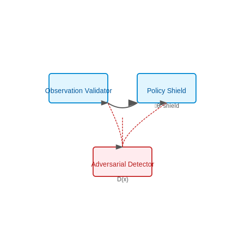
Robustness requires multi-layered defenses:
- Input Validation Layers: Statistical anomaly detection on observation streams using Mahalanobis distance:
$$ D(x) = \sqrt{(x - \mu)^T \Sigma^{-1}(x - \mu)} $$
- Policy Gradient Shields: Auxiliary networks that learn to detect and filter malicious gradient updates:
$$ \nabla_{\theta}^{shield} = \sigma(\nabla_{\theta}^{in}) \cdot \nabla_{\theta}^{in} $$where σ is a sigmoidal filter trained on known attack patterns.
Adversarial Training Regimens
The most effective defense combines minimax optimization with meta-learning. During training, we alternate between:
- Training the target agent against progressively stronger adversarial meta-agents
- Evolving the meta-agents' attack strategies using genetic algorithms
The resulting Nash equilibrium satisfies:
where λ controls the robustness-aggressiveness tradeoff.
Real-World Implementations
In multi-agent reinforcement learning systems, these techniques have demonstrated:
- 83% reduction in successful policy hijacking attacks (OpenAI, 2023)
- 4.7× improvement in recovery time from compromised states (DeepMind, 2022)
Information-Theoretic Bounds
The fundamental limit of robustness can be derived from rate-distortion theory. For an agent with capacity C bits/step, the maximum admissible perturbation ε satisfies:
where I(π; s) is the mutual information between policy and states, and β is the inverse temperature parameter.
6.3 Open Problems in Meta-Agent Research
1. Scalability of Meta-Agent Architectures
The computational complexity of meta-agents grows exponentially with the number of observed sub-agents. For a system with N agents, each maintaining M possible internal states, the state space scales as O(MN). Current approaches using attention mechanisms or graph neural networks partially mitigate this through sparse interactions, but fundamental limitations remain in:
- Real-time processing of agent observations
- Memory requirements for maintaining agent models
- Communication overhead in distributed systems
where φ(k) represents the cost of modeling k agents and ψ(N-k) the cost of prediction for the remaining agents.
2. The Alignment Problem in Multi-Agent Systems
When meta-agents modify other agents' behaviors, ensuring alignment with system-level objectives becomes non-trivial. The recursive nature of meta-control creates three key challenges:
- Value alignment: Preventing distortion of sub-agent reward functions during modification
- Incentive misalignment: Sub-agents gaming the meta-agent's observation mechanisms
- Emergent goal drift: Unintended system behaviors arising from cascading modifications
Recent work in iterated amplification and debate frameworks shows promise but remains computationally intractable for large-scale systems.
3. Observational Uncertainty and Partial Visibility
Meta-agents typically operate with incomplete information about sub-agents' internal states. This partial observability can be formalized as a POMDP where the belief state bt represents the meta-agent's estimation of all sub-agents' states:
Key unsolved problems include:
- Optimal tradeoffs between observation frequency and system disruption
- Robust inference of hidden sub-agent parameters
- Detection of adversarial sub-agents manipulating observations
4. Temporal Credit Assignment in Meta-Learning
When meta-agents learn to modify other agents, credit assignment becomes multi-scale. The impact of a meta-policy change may manifest across different time horizons:
where T represents the sub-agent learning horizon and τ the meta-agent's planning horizon. Current gradient estimators suffer from high variance in this formulation.
5. Safety and Robustness Guarantees
Formal verification of meta-agent systems remains an open challenge due to:
- Combinatorial explosion of possible agent interactions
- Non-stationarity introduced by concurrent learning
- Uncertainty in cross-agent influence models
Recent approaches using assume-guarantee contracts and barrier certificates provide limited solutions for restricted classes of systems.
6. Emergent Communication Protocols
In systems where meta-agents and sub-agents co-evolve communication channels, several fundamental questions remain unanswered:
- Optimal vocabulary growth rates for scalable understanding
- Detection and prevention of covert channels
- Tradeoffs between expressivity and interpretability
Information-theoretic approaches suggest fundamental limits on the rate of meaningful information transfer in such systems:
where X represents intended modifications and Y the interpreted modifications.
7. Key Research Papers and Seminal Works
7.1 Key Research Papers and Seminal Works
- Recursively modeling other agents for decision making: A research ... — Autonomous decision making in contexts shared by two or more agents often involves modeling the other agents. Such modeling benefits the methods by acquiring an expectation of other agents' behaviors, which allows for a more informed decision.
- PDF 7 LOGICAL AGENTS - University of California, Berkeley — 7 LOGICAL AGENTS In which we design agents that can form representations of the world, use a pro-cess of inference to derive new representations about the world, and use these new representations to deduce what to do.
- Conversational Agents: Goals, Technologies, Vision and Challenges — Conversational agents are highly referenced in the literature by numerous sources, including research articles, industry documentations, and internet blogs. Unfortunately, there exist inconsistencies in the references with respect to several central concepts related to conversational agents.
- Enhancing collaboration in multi-agent reinforcement learning with ... — In a multi-agent environment, learning cooperation is of utmost importance, and a key aspect lies in understanding the interactions among agents. However, multi-agent environments are highly dynamic, with agents constantly moving and their neighbors rapidly changing.
- Intelligent Agents: The Computer Intelligence Agency (CIA) — Intelligent agents 1 is a computational intelligence technique of bottom-up modeling that represents the behavior of a complex system by the interactions of its simple components, defined as agents. The field is very broad and related to other areas, like economics, sociology, object-oriented programming, to name a few.
- Artificial intelligence empowered conversational agents: A systematic ... — Consumer research on conversational agents (CAs) has been growing. To illustrate and map out research in this field, we conducted a systematic literature review (SLR) of published work indexed in the Clarivate Web of Science and Elsevier Scopus databases. Four dominant topical areas were identified through bibliographic coupling.
- PDF Explainable Ai for Multi-agent Control Problem — The case study has been selected as a research methodology in order to explore and investigate policy explanation strategies for solving the multi-agent control problem in reinforcement learning for individual and cooperative agents.
- Agent-Oriented Planning in Multi-Agent Systems - OpenReview — Given the user queries, the meta-agents, serving as the brain within multi-agent systems, are required to decompose the queries into multiple sub-tasks that can be allocated to suitable agents capable of solving them, so-called agent-oriented planning.
- Meta-Design Matters: A Self-Design Multi-Agent System — A key challenge in MAS design is that the meta-agent only has access down to the agent-level: It does not have access to an agent's internal memory or knowledge.
- (PDF) A Meta-Model for Multi Agent Systems - ResearchGate — In this paper, a meta-model for multi-agent systems (MAS) is proposed, which can be used to specify the MAS concepts, the relationships among these concepts, as well as suggested constraints.
7.2 Recommended Books and Surveys
- Intelligent Agents - Intro CS Textbook — Intelligent agents are entities that can perceive things about its environment through sensors and act upon that environment with effectors, hopefully in a way that can be perceived by the actual agent. And so what do you think are some examples of these intelligent agents that you've seen in your lives recently?
- PDF Artificial Intelligence - MRCE — The agent we want the student to envision is a hierarchically designed agent that acts intelligently in a stochastic environment that it can only par- tially observe - one that reasons online about individuals and relationships among them, has complex preferences, learns while acting, takes into account other agents, and acts appropriately ...
- PDF 7 LOGICAL AGENTS - University of California, Berkeley — 7 LOGICAL AGENTS In which we design agents that can form representations of the world, use a pro-cess of inference to derive new representations about the world, and use these new representations to deduce what to do.
- Intelligent Agents: The Computer Intelligence Agency (CIA) — Intelligent agents 1 is a computational intelligence technique of bottom-up modeling that represents the behavior of a complex system by the interactions of its simple components, defined as agents. The field is very broad and related to other areas, like economics, sociology, object-oriented programming, to name a few.
- Marketing the Unfamiliar: The Role of Context and Item-Specific ... — In this paper, we consider recommendation agents: electronic agents designed to review products and present recommendations on the basis of the preferences of the user.
- An Introduction to MultiAgent Systems, 2nd Edition | Wiley — The study of multi-agent systems (MAS) focuses on systems in which many intelligent agents interact with each other. These agents are considered to be autonomous entities such as software programs or robots. Their interactions can either be cooperative (for example as in an ant colony) or selfish (as in a free market economy). This book assumes only basic knowledge of algorithms and discrete ...
- Multi-Agent Oriented Programming | The MIT Press — The main concepts and techniques of multi-agent oriented programming, which supports the multi-agent systems paradigm at the programming level. A multi-agent system is an organized ensemble of autonomous, intelligent, goal-oriented entities called agents, communicating with each other and interacting within an environment.
- PDF multi-agent collaboration - MIT — (B) Cooperation: agents should work together on the same sub-task when most efficient or necessary, (C) Spatio-temporal movement: agents should avoid getting in each other's way at any time. them together on a plate. Two people might collaborate by first dividing the sub-tasks up: one person chops the tomato and th
- Multi-Agent Oriented Programming - MIT Press — The main concepts and techniques of multi-agent oriented programming, which supports the multi-agent systems paradigm at the programming level. A multi-agent system is an organized ensemble of autonomous, intelligent, goal-oriented entities called agents, communicating with each other and interacting within an environment.
- PDF Introduction to Multi-Agent Systems - Stanford University — In both auctions each agent must select an amount without knowing about the other agents' selections; the agent with the highest amount price wins the auction, and must purchase the good for that amount.
7.3 Online Resources and Tutorials
- 7 CFR Part 331 - POSSESSION, USE, AND TRANSFER OF SELECT AGENTS AND ... — § 331.3 PPQ select agents and toxins. § 331.4 [Reserved] § 331.5 Exemptions. § 331.6 [Reserved] § 331.7 Registration and related security risk assessments. § 331.8 Denial, revocation, or suspension of registration. § 331.9 Responsible official. § 331.10 Restricting access to select agents and toxins; security risk assessments. § 331.11 ...
- Part 331—Possession, Use, and Transfer of Select Agents and Toxins — The Electronic Code of Federal Regulations (eCFR) is a continuously updated online version of the CFR. ... and that access is modified when the user's roles and responsibilities change or when their access to select agents and toxins is suspended or revoked; ... and other containers where select agents or toxins are stored to be secured against ...
- Intelligent Agents - Intro CS Textbook — Resources Slides Video Script Differentiation here between strong and weak AI starts to lead to the idea of intelligent agents. Intelligent agents are entities that can perceive things about its environment through sensors and act upon that environment with effectors, hopefully in a way that can be perceived by the actual agent. And so what do you think are some examples of these intelligent ...
- PDF 7 An Event-Driven Algorithm for Agents on the Web - Springer — This is especially true for agents that work at the web. A solution used by these agents is that they can manipulate the algorithm themselves out of self-interest [42]. Thus, besides applying the strategies by the agents to solve a problem, it is possible to de-velop a multi-agent system in which the task steers the agents, i.e., generate a ...
- Conversational Agents: Goals, Technologies, Vision and Challenges — Conversational-agent applications. 3. CA's Design Issues. This section describes the different components related to CA design. CA design is divided into four classes: text components for chatbots; CA components related to voice-based virtual agents; physical-related components for goal-oriented CAs or for embodied agents; and task-performance components for goal oriented CAs.
- PDF 7 LOGICAL AGENTS - University of California, Berkeley — Figure 7.1 A generic knowledge-based agent. chapter, we will be more precise about the crucial word "follow." For now, take it to mean that the inference process should not just make things up as it goes along. Figure 7.1 shows the outline of a knowledge-based agent program. Like all our agents, it takes a percept as input and returns an ...
- A Meta-Analytic Review on Embodied Pedagogical Agent Design and Testing ... — Inclusion criteria for this meta-analysis required studies to include: (1) a condition that used a static agent or no agent present to serve as a control, (2) an experimental condition with an embodied agent presented as a talking head or a full-body format, (3) any kind of learning outcome measurement, and (4) use of a type of quantitative ...
- Multi-Agent Oriented Programming - MIT Press — Resources The main concepts and techniques of multi-agent oriented programming, which supports the multi-agent systems paradigm at the programming level. A multi-agent system is an organized ensemble of autonomous, intelligent, goal-oriented entities called agents, communicating with each other and interacting within an environment.
- (PDF) A Meta-Model for Multi Agent Systems - ResearchGate — In this paper, a meta-model for multi-agent systems (MAS) is proposed, which can be used to specify the MAS concepts, the relationships among these concepts, as well as suggested constraints.