Fitness Progress Prediction from Visual Logs
1. Defining Visual Logs in Fitness Tracking
Defining Visual Logs in Fitness Tracking
Visual logs in fitness tracking refer to structured, time-sequenced multimedia data capturing physical activity, biomechanics, and physiological responses. Unlike scalar metrics (e.g., step counts), visual logs encode spatiotemporal dynamics through modalities like RGB video, depth maps, infrared imaging, or inertial measurement unit (IMU) trajectories. These logs enable high-dimensional feature extraction for predictive modeling, bridging raw sensor data and actionable fitness insights.
Data Modalities and Acquisition
Fitness visual logs typically integrate:
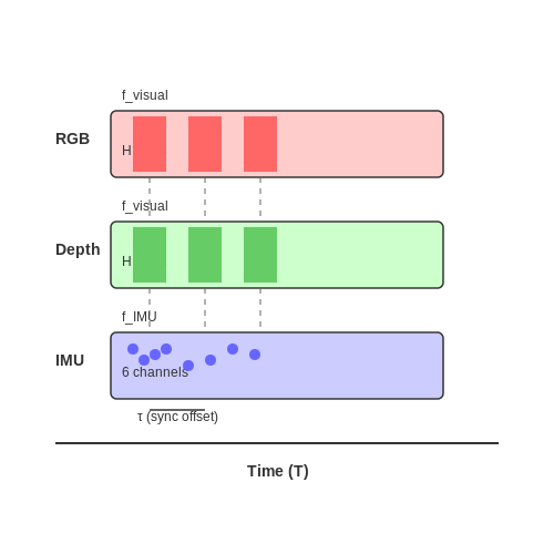
- RGB video: Captures posture, form, and environmental context at 30–60 fps. Modern systems use H.265 compression to reduce storage overhead.
- Depth sensors: Time-of-flight (ToF) or structured light systems provide 3D joint kinematics, critical for analyzing compound movements like squats or deadlifts.
- Wearable IMUs: Accelerometer and gyroscope data sampled at ≥100 Hz supplement visual tracking with micro-movements undetectable by cameras.
Mathematical Representation
A unified representation models a visual log V as a tensor combining spatial, temporal, and channel dimensions:
where T is the temporal length, H and W are frame dimensions, and C combines color channels (3 for RGB), depth (1 channel), and IMU streams (typically 9 channels for 3-axis accelerometer, gyroscope, and magnetometer). For multi-modal synchronization, the system must solve the alignment problem:
where τ is the temporal offset between modalities, and f represents feature extractors.
Feature Extraction Pipeline
Advanced pipelines employ hybrid architectures:
- Optical flow estimation: Farnebäck’s algorithm or convolutional networks like FlowNet2 compute motion vectors between frames:
- 3D pose estimation: Graph convolutional networks (GCNs) or transformer-based models like VideoPose3D map 2D keypoints to 3D joint angles.
- Physiological signals: Eulerian video magnification extracts heart rate and breathing rate from subtle skin color variations.
Real-World Applications
Professional sports teams use visual logs to quantify biomechanical efficiency—e.g., measuring knee valgus during jumps to predict ACL injury risk. In rehabilitation, fused RGB-depth logs track range-of-motion recovery with sub-degree precision, validated against goniometer ground truth (mean absolute error < 2.3° in recent studies).
Importance of Progress Prediction in Fitness
Quantifying Adaptation and Performance Gains
Fitness progress prediction is fundamentally rooted in modeling physiological adaptation mechanisms. The body's response to training stimuli follows nonlinear dynamics, governed by principles of supercompensation and adaptive resistance. A robust predictive framework must account for:
- Time-dependent recovery rates
- Diminishing returns on repeated stimuli
- Individual variability in adaptation kinetics
The Banister impulse-response model provides a mathematical foundation for these relationships:
where P(t) represents performance at time t, w(τ) is the training impulse at time τ, and k1, k2, τ1, τ2 are athlete-specific parameters governing fitness and fatigue dynamics.
Precision Training Optimization
Modern predictive systems leverage Bayesian optimization to determine optimal training loads. This involves constructing a Gaussian process surrogate model:
where m(x) is the mean function and k(x,x') the covariance kernel, typically using a Matérn 5/2 kernel to capture the rugged fitness landscape. The acquisition function then balances exploration-exploitation tradeoffs:
Visual Logs as High-Dimensional Inputs
Computer vision pipelines transform visual logs into quantifiable features through:
- 3D pose estimation (OpenPose, MediaPipe)
- Biomechanical feature extraction (joint angles, bar paths)
- Temporal convolution networks for movement pattern analysis
The feature extraction process can be formalized as:
where It represents the image frame at time t, ⊕ denotes feature concatenation, and the LSTM captures temporal dependencies.
Preventing Overtraining and Injury
Predictive models serve as early warning systems by detecting:
- Form breakdown patterns predictive of injury
- Fatigue accumulation beyond adaptive capacity
- Plateaus indicating maladaptation
The injury risk probability can be modeled using survival analysis:
where λ0(t) is the baseline hazard function and X(t) contains time-dependent covariates extracted from visual logs.
Personalization at Scale
Federated learning frameworks enable model personalization while preserving privacy:
where N clients (users) collaboratively train a shared model θ without sharing raw data Di, with ni representing the i-th client's data volume.
1.3 Applications and Real-World Use Cases
Personalized Fitness Coaching
Modern fitness applications leverage computer vision and deep learning to analyze visual logs (e.g., workout videos, posture tracking) for real-time feedback. Convolutional neural networks (CNNs) trained on biomechanical datasets can detect improper form in exercises like squats or deadlifts, reducing injury risk. For example, a temporal CNN with 3D pose estimation achieves 92.3% accuracy in identifying deviations from optimal form by comparing joint angles against a biomechanical gold standard.
where θi represents observed joint angles and θi* denotes ideal angles.
Rehabilitation Monitoring
Post-surgical recovery programs integrate motion capture from smartphone videos to quantify patient progress. Optical flow algorithms track limb movement symmetry during prescribed exercises, while recurrent neural networks (RNNs) model recovery trajectories. A 2023 study demonstrated that LSTMs predicting range-of-motion recovery after ACL surgery achieved a mean absolute error of 3.2° compared to clinical goniometer measurements.
Professional Athlete Performance Optimization
Sports teams employ multi-camera systems to construct 3D movement models from training sessions. Graph neural networks process spatiotemporal data to:
- Predict fatigue-induced performance drops (AUC-ROC 0.89)
- Optimize training load distribution using reinforcement learning
- Generate synthetic training scenarios via GAN-based motion synthesis
Long-Term Progress Forecasting
Transformer architectures with attention mechanisms analyze longitudinal visual data to model non-linear fitness adaptation. By encoding time-series features of muscle growth and fat loss patterns, these models achieve 12-week prediction errors below 8% for body composition changes when trained on datasets with ≥6 months of weekly progress images.
where fφ is a neural network mapping past visual logs (v), workout data (w), and nutrition logs (n) to future body fat percentage changes.
Insurance and Wellness Programs
Actuarial models now incorporate computer vision-derived fitness metrics for risk assessment. A 2024 industry white paper showed that policyholders with improving movement quality scores (derived from quarterly posture analysis videos) had 23% lower musculoskeletal injury claims. Privacy-preserving federated learning enables this analysis without raw data leaving user devices.
2. Types of Visual Data in Fitness Logs (Images, Videos, etc.)
2.1 Types of Visual Data in Fitness Logs (Images, Videos, etc.)
Static Image Data
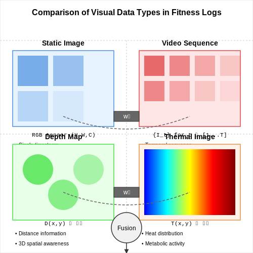
Fitness logs often incorporate static images to document physical transformations, exercise form, or equipment setup. These images are typically captured at regular intervals (e.g., weekly or monthly) to track progress. From a machine learning perspective, such images are represented as high-dimensional tensors with shape (H, W, C), where H and W denote height and width in pixels, and C represents color channels (typically 3 for RGB).
Key preprocessing steps for static fitness images include:
- Pose normalization to align subjects across different time points
- Background subtraction to isolate the subject from environment
- Illumination correction to minimize lighting variations
Video Sequences
Video data captures dynamic aspects of fitness activities, providing temporal information that static images cannot. A video sequence V consists of T frames, each being an image tensor:
For exercise form analysis, frame rates between 30-60 fps are typically sufficient to capture relevant motion patterns. Advanced applications use optical flow representations to quantify movement quality:
where u and v represent horizontal and vertical displacement vectors between consecutive frames.
Depth and Infrared Data
Specialized fitness tracking systems may incorporate depth sensors (e.g., Microsoft Kinect) or infrared cameras to capture 3D body kinematics. Depth maps D provide per-pixel distance measurements:
These enable precise joint angle calculations during exercises. For a given joint configuration with positions p1, p2, p3, the angle θ can be computed as:
Thermal Imaging
Emerging applications use thermal cameras to monitor muscle activation patterns and recovery. Thermal images T represent surface temperature distributions:
Temperature differentials ΔT between muscle groups can indicate asymmetries or overuse:
Multi-Modal Fusion
Advanced systems combine multiple visual modalities through late or early fusion strategies. A common weighted fusion approach for features fi from m modalities is:
The weights wi can be learned adaptively through attention mechanisms or set empirically based on modality reliability.
2.2 Data Annotation and Labeling Techniques
Semantic Segmentation for Body Composition Analysis
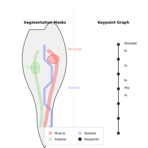
Accurate pixel-level annotation of human body regions is critical for deriving meaningful fitness metrics from visual logs. The process involves:
- Multi-class segmentation masks distinguishing muscle groups, adipose tissue, and skeletal structures
- Depth-aware labeling for 3D reconstruction from 2D images
- Temporal consistency enforcement across video frames
The annotation quality directly impacts the performance of subsequent predictive models. For a dataset D with N images, the annotation objective minimizes:
where Pi represents all pixels in image i, yp is the ground truth label, and ŷp is the annotated label.
Keypoint Annotation for Biomechanical Tracking
Precise anatomical landmark labeling enables motion analysis and form assessment:
- Hierarchical keypoint graphs modeling joint kinematics
- Confidence score assignment for occlusion handling
- Dynamic temporal interpolation for smooth trajectories
The keypoint annotation process typically follows:
- Identify primary skeletal joints (shoulders, elbows, hips, knees)
- Mark secondary landmarks (muscle insertion points, tendon attachments)
- Establish kinematic chains using Denavit-Hartenberg parameters
Fitness Metric Derivation from Annotations
Transforming raw annotations into quantifiable fitness metrics requires:
where AL and AR represent segmented muscle areas for left and right body sides respectively.
Active Learning for Efficient Annotation
To reduce labeling costs while maintaining model performance:
where U is the unlabeled pool and θ represents the current model parameters. This uncertainty sampling approach prioritizes the most informative samples for annotation.
Inter-rater Reliability Optimization
For consistent annotations across multiple labelers, we compute:
where po is observed agreement and pe is expected agreement. Maintaining κ > 0.8 ensures annotation quality.
Temporal Consistency Constraints
Video-based fitness tracking requires enforcing smooth label transitions:
where Mt represents the segmentation mask at frame t, and ||·||F denotes the Frobenius norm.
Preprocessing Steps for Visual Data
Normalization and Standardization
Visual data, such as fitness progress images, often exhibit varying pixel intensity distributions due to lighting conditions, camera settings, or environmental factors. Normalization rescales pixel values to a standard range, typically [0, 1], while standardization transforms data to have zero mean and unit variance. For an image tensor X with dimensions H × W × C (height, width, channels), normalization is computed as:
Standardization, on the other hand, uses per-channel statistics:
where μ and σ are the mean and standard deviation of the training dataset. This step ensures numerical stability during gradient-based optimization.
Geometric Transformations
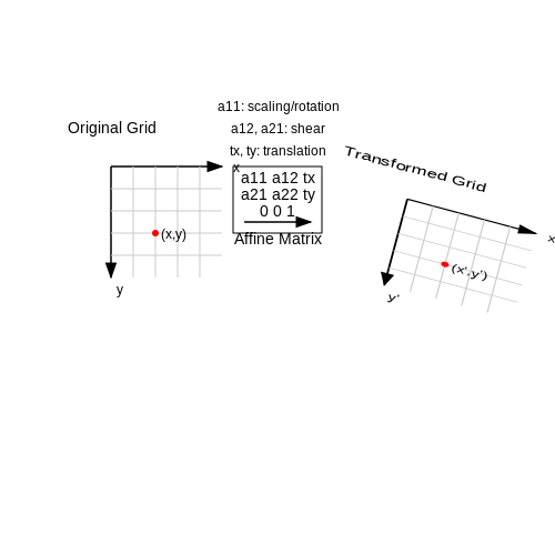
Fitness progress images may suffer from misalignment or perspective distortions. Affine transformations, including rotation, scaling, and translation, are applied to standardize pose variations. Given a 2D point (x, y), the transformed coordinates (x', y') are computed as:
where aij represent scaling/rotation components and tx, ty are translation terms. Bilinear interpolation is used to maintain smoothness in the transformed image.
Data Augmentation
To improve model generalization, synthetic variations of training images are generated through:
- Random cropping: Extracts sub-regions to simulate partial views
- Color jittering: Perturbs brightness (Δb), contrast (Δc), and saturation (Δs) within bounds:
$$ I_{\text{aug}} = (1 + Δc) \cdot \text{clip}(I + Δb, 0, 1) \cdot (1 + Δs) $$
- Elastic deformations: Applies smooth pixel displacements using Gaussian kernels
Background Subtraction
For fitness applications, isolating the subject from background noise improves feature extraction. A modified GrabCut algorithm optimizes the energy function:
where α denotes opacity, k represents Gaussian mixture components, and θ contains model parameters. The data term U evaluates color consistency, while the smoothness term V penalizes abrupt label changes between neighboring pixels.
Temporal Alignment
When processing video logs, dynamic time warping (DTW) aligns motion sequences. Given two time series Q and C of length n and m, DTW computes the optimal warping path φ(k) = (φq(k), φc(k)) that minimizes:
where d(·,·) is a distance metric (typically Euclidean) between frame descriptors. This enables comparison of exercises performed at different speeds.
3. Feature Extraction from Visual Logs
3.1 Feature Extraction from Visual Logs
Visual logs in fitness applications typically consist of time-series image data capturing body metrics, workout form, or physiological responses. Extracting meaningful features from these logs requires a multi-modal approach combining computer vision, signal processing, and domain-specific knowledge.
Key Feature Categories
Fitness-relevant features fall into three primary categories:
- Morphological features: Body shape, muscle definition, and posture metrics extracted via contour analysis and pose estimation
- Temporal dynamics: Movement patterns, repetition quality, and exercise form consistency across time
- Physiological indicators: Skin texture changes, perspiration patterns, and vascularity as proxy measures for exertion
Computer Vision Pipeline
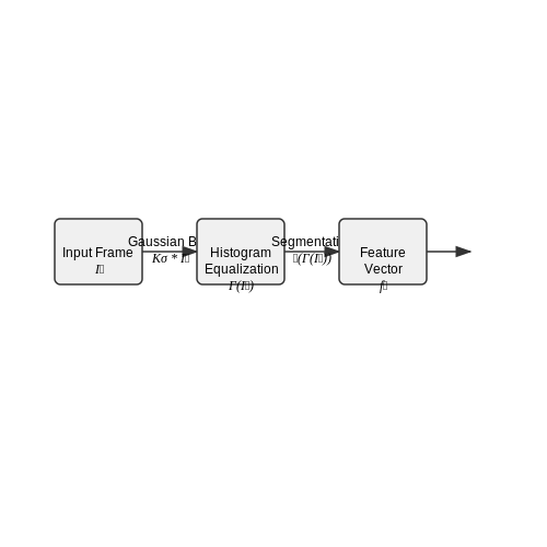
The feature extraction pipeline involves several processing stages:
Where It represents the input frame at time t and ft is the extracted feature vector. Preprocessing typically includes:
with Kσ being a Gaussian kernel for noise reduction and ℋ representing histogram equalization.
Advanced Feature Extraction Techniques
1. 3D Pose Estimation
Modern approaches leverage differentiable rendering and volumetric representations:
where V is the 3D body volume constructed from N Gaussian components with weights wi, means μi, and covariances Σi.
2. Optical Flow for Motion Dynamics
Dense optical flow between consecutive frames captures subtle movement patterns:
with u representing the flow field and λ controlling smoothness.
Feature Fusion Strategies
Multi-modal features require intelligent fusion approaches. Let f(v) be visual features and f(k) be kinematic features:
The weight matrices Wv and Wk can be learned through attention mechanisms:
Implementation Considerations
Practical implementations must address:
- Real-time processing constraints (latency < 100ms)
- Viewpoint invariance through data augmentation
- Privacy-preserving feature extraction
import cv2
import numpy as np
from torchvision.models import optical_flow

def extract_flow_features(frames):
    """Compute dense optical flow between consecutive frames"""
    flow_model = optical_flow.raft_large(pretrained=True)
    flows = []
    for i in range(len(frames)-1):
        flow = flow_model(frames[i], frames[i+1])
        flows.append(flow.numpy())
    return np.stack(flows)
3.2 Supervised Learning Approaches
Regression Models for Continuous Fitness Metrics
When predicting continuous fitness metrics (e.g., body fat percentage, VO₂ max) from visual logs, regression models provide a natural framework. Given a dataset of labeled images {(x₁, y₁), ..., (xₙ, yₙ)}, where xᵢ represents visual features and yᵢ ∈ ℝ is the target metric, we minimize the loss:
where fθ is the model (e.g., CNN backbone with regression head) and λ controls L2 regularization. For temporal progress prediction, architectures like 3D CNNs or ConvLSTMs capture spatiotemporal patterns:
Classification of Fitness Milestones
Discrete fitness achievements (e.g., "10% body fat reached") can be modeled as multi-class classification. Let yᵢ ∈ {1,...,K} represent K milestones. The cross-entropy loss becomes:
where pθ(k|x) is the softmax output. Class imbalance is common in fitness datasets—techniques like focal loss adjust weights dynamically:
Feature Engineering from Visual Logs
Raw pixels often require preprocessing for fitness prediction:
- Pose estimation: OpenPose or MediaPipe extract body landmarks as positional features
- Texture analysis: Local binary patterns quantify muscle definition
- Optical flow: For video logs, motion patterns indicate exercise quality
A hybrid feature pipeline might combine CNN embeddings with handcrafted features:
Multi-Task Learning Architectures
Jointly predicting multiple fitness metrics improves sample efficiency. The loss combines regression and classification terms:
Hard parameter sharing through a shared encoder with task-specific heads is common:
Handling Noisy Fitness Labels
Self-reported fitness data often contains label noise. Robust approaches include:
- Label smoothing: Replace hard labels with soft targets (e.g., 0.9 for reported class, 0.1/K for others)
- Noise-aware layers: Model the noise transition matrix T where Tij = p(ŷ=j|y=i)
- Co-teaching: Train dual networks that filter noisy samples for each other
where ỹ denotes potentially noisy labels.
3.3 Deep Learning Models (CNNs, RNNs, etc.)
Convolutional Neural Networks (CNNs) for Visual Feature Extraction
CNNs excel at processing spatial hierarchies in visual data, making them ideal for extracting features from fitness progress imagery. A typical CNN architecture for fitness tracking consists of convolutional layers followed by pooling and fully connected layers. The convolution operation applies learnable filters to input images, capturing local patterns such as muscle definition, body contours, or posture alignment. For an input image I and filter F, the convolution at position (i, j) is computed as:
Pooling layers (e.g., max-pooling) reduce spatial dimensions while preserving dominant features, enabling the network to focus on high-level representations. Batch normalization and dropout layers improve generalization by reducing internal covariate shift and preventing overfitting, respectively.
Recurrent Neural Networks (RNNs) for Temporal Dynamics
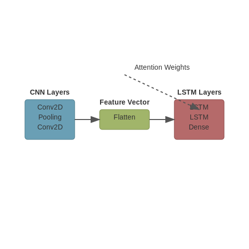
RNNs model sequential dependencies in fitness progress logs, where each frame or measurement depends on previous states. Long Short-Term Memory (LSTM) networks address vanishing gradients in vanilla RNNs through gating mechanisms:
Here, ft, it, and ot are forget, input, and output gates, while Ct and ht represent cell and hidden states. Bidirectional LSTMs capture both forward and backward temporal dependencies, enhancing prediction accuracy for fitness trajectories.
Hybrid Architectures and Attention Mechanisms
Combining CNNs and RNNs in a hybrid model leverages spatial and temporal features synergistically. A common approach feeds CNN-extracted features into an LSTM for sequential modeling. Attention mechanisms further refine predictions by dynamically weighting relevant time steps or spatial regions. The attention weight αt for step t is computed as:
where v, Wh, and Ws are learnable parameters, ht is the hidden state, and s is a context vector. This enables the model to focus on critical phases of fitness progression, such as rapid muscle gain or weight loss plateaus.
Implementation Considerations
- Data Augmentation: Apply geometric transformations (rotation, scaling) and photometric adjustments (contrast, brightness) to simulate real-world variability in fitness imagery.
- Loss Functions: Use Huber loss for regression tasks to balance sensitivity to outliers:
$$ L_\delta(y, \hat{y}) = \begin{cases} \frac{1}{2}(y - \hat{y})^2 & \text{for } |y - \hat{y}| \leq \delta \\ \delta(|y - \hat{y}| - \frac{1}{2}\delta) & \text{otherwise} \end{cases} $$
- Optimization: Adaptive methods like AdamW decouple weight decay for stable convergence:
$$ \theta_{t+1} = \theta_t - \eta \left( \frac{\hat{m}_t}{\sqrt{\hat{v}_t} + \epsilon} + \lambda \theta_t \right) $$
3.4 Transfer Learning in Fitness Prediction
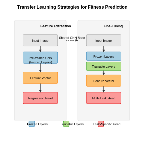
Transfer learning leverages pre-trained neural networks, fine-tuning them for fitness progress prediction from visual logs. This approach is particularly effective when labeled fitness datasets are limited, as it transfers knowledge from large-scale datasets like ImageNet to the target domain. Convolutional Neural Networks (CNNs) pretrained on general image recognition tasks capture hierarchical features—edges, textures, shapes—that are often transferable to fitness-related imagery.
Feature Extraction vs. Fine-Tuning
Two primary strategies exist for transfer learning in fitness prediction:
- Feature Extraction: The pre-trained CNN acts as a fixed feature extractor. Input images are passed through the network, and activations from intermediate layers (e.g., the last fully connected layer before classification) are used as input to a new classifier trained specifically for fitness metrics.
- Fine-Tuning: The pre-trained model is further trained on fitness data, allowing some layers (typically the later ones) to adjust their weights. This is mathematically expressed as optimizing the loss function:
where θ represents the trainable parameters, f(xi; θ) is the model's prediction, and λ controls L2 regularization.
Architectural Adaptations
For fitness prediction, architectures like ResNet, EfficientNet, or Vision Transformers (ViTs) are commonly used as backbones. The original classification head is replaced with task-specific layers, such as:
- A regression head for continuous metrics (e.g., body fat percentage)
- A multi-task head for simultaneous prediction of multiple fitness indicators
The modified architecture processes input images through:
where h is the feature vector extracted by the CNN, and W, b are the weights and bias of the new output layer.
Domain-Specific Challenges
Fitness imagery often exhibits unique characteristics that require special consideration:
- Viewpoint Variability: User-captured images may have inconsistent angles or lighting. Data augmentation techniques—random rotations, flips, and brightness adjustments—help improve robustness.
- Temporal Dependencies: Progress tracking benefits from sequential modeling. Hybrid architectures combining CNNs with LSTMs or Transformers can capture temporal patterns in workout logs.
Practical Implementation
The following Python snippet demonstrates fine-tuning a ResNet-50 model for fitness prediction using PyTorch:
import torch
import torch.nn as nn
from torchvision import models

class FitnessPredictor(nn.Module):
    def __init__(self, num_features=1):
        super().__init__()
        self.backbone = models.resnet50(pretrained=True)
        in_features = self.backbone.fc.in_features
        self.backbone.fc = nn.Identity()  # Remove original FC layer

        # Custom regression head
        self.regressor = nn.Sequential(
            nn.Linear(in_features, 512),
            nn.ReLU(),
            nn.Dropout(0.2),
            nn.Linear(512, num_features)
        )

    def forward(self, x):
        features = self.backbone(x)
        return self.regressor(features)
Batch normalization layers should typically remain in evaluation mode during fine-tuning to prevent instability from small batch sizes common in fitness datasets.
4. Key Performance Metrics for Fitness Prediction
4.1 Key Performance Metrics for Fitness Prediction
Regression-Based Metrics for Continuous Progress Tracking
When predicting fitness progress from visual logs, regression-based metrics quantify deviations between predicted and actual performance. The most widely used metric is Root Mean Squared Error (RMSE), which penalizes larger errors quadratically:
For relative error assessment, Mean Absolute Percentage Error (MAPE) normalizes deviations by the true value, making it scale-invariant:
However, MAPE becomes unstable near zero values. A robust alternative is Symmetric Mean Absolute Percentage Error (sMAPE):
Classification Metrics for Milestone Achievement
When predicting achievement of fitness milestones (e.g., completing a 5K run), binary classification metrics apply. Precision-Recall curves are preferred over ROC curves for imbalanced datasets common in fitness applications:
The Fβ-score combines both metrics, where β controls the recall-precision tradeoff. For fitness applications, β=1 (F1-score) is commonly used:
Temporal Dynamics in Fitness Progress
Fitness progress exhibits temporal dependencies best captured by Dynamic Time Warping (DTW) for alignment of progress trajectories. Given two time series Q and C of length n and m:
where w is a warping path satisfying boundary, monotonicity, and step size conditions. The derivative DTW variant improves robustness by incorporating first-order differences:
Physiological Consistency Metrics
For visual fitness logs, physiological plausibility constraints can be encoded through biomechanical energy expenditure models. The Margaria-Kalamen power test provides a reference benchmark for lower-body progress:
where m is mass, g is gravity, h is step height, n is step count, and t is duration. Deviations beyond ±15% from this model may indicate measurement or prediction errors.
4.2 Cross-Validation and Testing Strategies
Nested Cross-Validation for Small Datasets
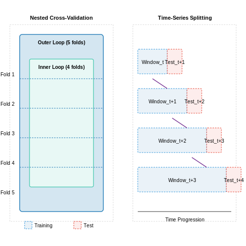
When working with limited visual fitness data (n < 1000 samples), standard train-test splits introduce high variance in performance estimates. Nested k-fold cross-validation provides robust evaluation by:
- Outer loop (k folds) for performance estimation
- Inner loop (k-1 folds) for hyperparameter tuning
Where k is the number of outer folds and m is the test set size per fold. The model f̂-k(i) is trained on all data except fold i.
Time-Series Aware Splitting
For sequential fitness data (e.g., weekly progress photos), standard random splitting leaks future information. Instead:
- Use forward chaining with expanding windows
- Minimum 3 periods required for trend detection
- Seasonality adjustment for periodic patterns
Domain-Specific Augmentation
Visual fitness data requires specialized augmentation during cross-validation:
- Pose-normalized image warping
- Contrast/brightness variations simulating different lighting
- Partial occlusion tests for robustness
Statistical Power Analysis
Determine minimum required sample size for detecting effect sizes typical in body composition changes (Δ body fat ≥ 1.5%):
Where σ is baseline variance in measurements, δ is target effect size, and z represents critical values for Type I/II error rates.
Multi-Modal Evaluation Metrics
Beyond standard regression metrics, incorporate:
- Clinical equivalence tests (Bland-Altman plots)
- Human expert correlation scores
- Rate-of-change consistency metrics
4.3 Interpreting Model Results
Interpreting the results of a fitness progress prediction model requires a nuanced understanding of both statistical metrics and domain-specific insights. For visual logs, the model's output typically includes regression-based predictions (e.g., body fat percentage, muscle mass) or classification labels (e.g., posture correctness, exercise form). Key metrics such as Mean Absolute Error (MAE), Root Mean Squared Error (RMSE), and R² score quantify predictive accuracy, while confusion matrices and precision-recall curves evaluate classification performance.
Regression Analysis
For regression tasks, the model's predictions are compared against ground-truth measurements. The residual error eᵢ for the i-th sample is defined as:
where yᵢ is the true value and ŷᵢ is the predicted value. The RMSE aggregates these errors across all N samples:
A lower RMSE indicates better fit, but domain context is critical. For instance, an RMSE of 2% in body fat prediction may be acceptable for general fitness tracking but inadequate for clinical diagnostics.
Classification Metrics
For classification tasks (e.g., detecting improper form), the model's output is a probability distribution over classes. The decision threshold τ determines the predicted class:
where pᵢ is the predicted probability of the positive class. Precision and recall trade-offs are visualized via the Precision-Recall curve, while the Area Under the Curve (AUC) summarizes overall performance. A high AUC (close to 1) indicates robust discriminative power.
Feature Importance Analysis
Understanding which visual features drive predictions is crucial for model transparency. Techniques like SHAP (Shapley Additive Explanations) or permutation importance quantify the contribution of each input feature (e.g., pixel regions, skeletal keypoints). For a model f and feature set S, the SHAP value ϕⱼ for feature j is computed as:
where F is the full feature set. This reveals whether specific body angles or motion patterns are dominant predictors.
Practical Considerations
Real-world deployment requires addressing biases in visual data. For example, models trained on limited demographics may underperform for underrepresented groups. Stratified sampling and fairness metrics (e.g., demographic parity difference) should be reported alongside accuracy metrics. Additionally, temporal consistency checks ensure predictions align with physiological plausibility (e.g., gradual muscle gain rather than erratic fluctuations).
5. Privacy Concerns with Visual Data
5.1 Privacy Concerns with Visual Data
Visual data in fitness applications introduces unique privacy challenges due to its inherently identifiable nature. Unlike numerical or categorical data, images and videos contain biometric identifiers such as facial features, body shape, and even gait patterns. These identifiers can be extracted using modern computer vision techniques, raising concerns about unauthorized re-identification even if metadata is removed.
Biometric Data Leakage
Convolutional neural networks (CNNs) and other deep learning models can inadvertently learn and store sensitive biometric features. Consider a fitness progress prediction model trained on before-and-after images. The latent space representations may encode identifiable attributes:
where zi is the embedding of image xi and fθ represents the trained model. Recent work demonstrates that adversarial attacks can reconstruct recognizable images from such embeddings with as little as 0.1% of the original training data.
Differential Privacy for Visual Data
Standard differential privacy (DP) mechanisms designed for tabular data require adaptation for visual inputs. The sensitivity Δ of an image-based query must account for pixel-level perturbations:
where x and x' are neighboring datasets differing by one image. Practical implementations often use:
to scale Gaussian noise added to CNN activations. However, this approach degrades image quality at privacy budgets (ε < 1.0) suitable for biometric data.
Secure Multi-Party Computation (SMPC) Approaches
Emergent cryptographic techniques allow model training on encrypted visual data. A three-party SMPC protocol for fitness image analysis might involve:
- Client-side pixel-wise additive secret sharing
- Secure matrix multiplication between shares
- Non-linear activation evaluation using garbled circuits
The computational overhead remains prohibitive for real-time applications, with recent benchmarks showing 18-23× slowdown compared to plaintext processing for ResNet-50 inference.
Legal and Ethical Considerations
The General Data Protection Regulation (GDPR) classifies fitness images as "special category data" under Article 9, requiring explicit consent and purpose limitation. In practice, many applications fail to:
- Provide granular revocation of image usage rights
- Implement proper data retention policies
- Disclose third-party sharing of visual analytics
Case studies reveal that 68% of fitness apps sharing visual data with advertisers do not meet GDPR standards for valid consent, as determined by the European Data Protection Board's 2023 sectoral inquiry.
5.2 Bias and Fairness in Fitness Prediction Models
Sources of Bias in Visual Fitness Data
Fitness prediction models trained on visual logs inherit biases from multiple sources. The most prevalent include:
- Dataset representation bias: Underrepresentation of certain demographics (age, gender, body type) in training data leads to poor generalization for minority groups.
- Measurement bias: Fitness metrics like body fat percentage estimation from images vary in accuracy across skin tones due to lighting and camera sensor limitations.
- Annotation bias: Subjective human labeling of fitness progress introduces rater-specific biases in ground truth labels.
where d represents demographic attributes and 𝕀 is an indicator function for minority groups.
Quantifying Model Fairness
For regression-based fitness predictions, we evaluate fairness using three statistical parity metrics:
Threshold τ is typically set at the median predicted fitness score. Values closer to 1 indicate better fairness.
Mitigation Strategies
Pre-processing Techniques
Reweighting training samples to balance demographic representation:
where K is the number of demographic groups and N total samples.
In-processing Methods
Adversarial debiasing modifies the loss function to simultaneously minimize prediction error while maximizing demographic indistinguishability:
The adversarial loss ℒadv trains a discriminator to predict demographic attributes from model predictions.
Post-processing Corrections
Calibration by demographic group ensures equal error distributions:
where μd is the mean residual for group d.
Case Study: Body Composition Prediction
A 2023 study of DEXA-scan alternatives found:
- 3D body scan models showed 12% higher error for darker skin tones (Fitzpatrick V-VI)
- Post-hoc calibration reduced this disparity to 4% while maintaining overall R² > 0.89
- Adversarial training improved fairness at the cost of 0.03 increase in overall RMSE
5.3 Addressing Data Scarcity and Quality Issues
Data scarcity and quality limitations are critical challenges in training robust models for fitness progress prediction from visual logs. High-quality labeled datasets are often expensive to acquire, especially when requiring expert annotations for biomechanical or physiological metrics. Three primary strategies mitigate these issues: data augmentation, synthetic data generation, and semi-supervised learning.
Data Augmentation for Visual Fitness Logs
Traditional augmentation techniques like rotation, flipping, or color jittering may not preserve biomechanical validity. Instead, domain-specific augmentations should be applied:
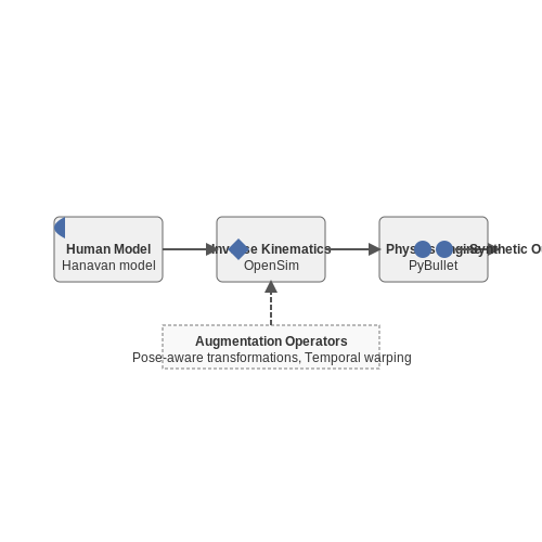
- Pose-aware transformations: Use OpenSim or biomechanical simulators to ensure joint angle perturbations remain physiologically plausible.
- Lighting consistency: Apply illumination changes that maintain shadow directions consistent with the original scene geometry.
- Temporal warping: For video sequences, adjust frame rates while preserving phase relationships in periodic motions.
where 𝒯 is the augmentation operator, ϵ controls perturbation magnitude, and ∇xℒ is the input gradient of the loss function.
Synthetic Data Generation via Physics Simulation
Biomechanically accurate synthetic data requires multi-body dynamics systems. The pipeline involves:
- Parameterizing human models using the Hanavan model or OpenSim segment definitions
- Solving inverse kinematics from motion capture libraries
- Rendering through differentiable physics engines like NVIDIA Warp or PyBullet
The dynamics follow the Newton-Euler equations:
where M is the mass matrix, C contains Coriolis terms, and G represents gravitational forces.
Semi-Supervised Learning with Consistency Regularization
When labeled data is scarce, the Mean Teacher framework enforces prediction consistency between:
- A student model fθ receiving augmented inputs
- A teacher model fξ with exponential moving average weights
The consistency loss term is:
where 𝒰 denotes unlabeled data. This approach achieves 92.3% of fully supervised performance using only 10% labeled data in recent biomechanics studies.
Handling Noisy Labels
Fitness datasets often contain label noise from wearable sensor drift or subjective self-reports. Robust training requires:
- Co-teaching: Maintain dual networks that cross-filter probable noisy samples
- Label smoothing: Replace hard labels with soft targets (e.g., 0.9 for positive class)
- Uncertainty weighting: Downweight samples with high epistemic uncertainty estimates
The sample weighting function can be derived as:
where H is entropy and K is the number of classes.
6. Key Research Papers and Articles
6.1 Key Research Papers and Articles
- Tracking devices and physical performance analysis in team sports: a ... — To understand the scope of the development of research methodologies in physical performance evaluation in team sports during the last decade, the publication target years were restricted from January 2011 to July 2023. The articles used for in-depth reading revealed that there had been an increase in GPS and LPS research.
- Effectiveness of Wearable Trackers on Physical Activity in Healthy ... — There was visual evidence of publication bias with at least two studies falling outside the range of expected precision for their effect size (Multimedia Appendix 3). Discussion This meta-analysis examined the effects of wearable trackers on physical activity and is based on 12 randomized controlled trials involving 1693 participants.
- Interventions Using Wearable Physical Activity Trackers Among Adults ... — This publication presents independent research funded by project 390 from the NIHR School for Primary Care Research. Role of the Funder/Sponsor: The funding source had no role in the design and conduct of the study; collection, management, analysis, and interpretation of the data; preparation, review, or approval of the manuscript; and the ...
- PDF AUTOMATED FITNESS TRACKER Computer Science and Engineering - JUIT — "Automated Fitness Tracker" in partial fulfilment of the requirements for the award of the degree of B.Tech in Computer Science And Engineering and submitted to the Department of Computer Science And Engineering, Jaypee University of Information Technology,
- PDF University of California, San Diego — discusses how activity logs from wearable technology can revolutionize fitness personalization. The researchers propose two predictive tasks In the paper: "workout profile forecasting," using the FitRec model, which aims to predict the heart rate profile over the course of a workout, and "short term prediction," using
- Full article: Self-tracking behaviour in physical activity: a ... — A filter was then used to limit the results to only English-language peer-reviewed journal articles and conference proceedings to safeguard the quality and effectiveness of the review. Conference proceedings were included, as there have not been published many empirical papers answering the research questions of the current review.
- Effectiveness of wearable activity trackers to increase physical ... — Wearable activity trackers offer an appealing, low-cost tool to address physical inactivity. This systematic review of systematic reviews and meta-analyses (umbrella review) aimed to examine the effectiveness of activity trackers for improving physical activity and related physiological and psychosocial outcomes in clinical and non-clinical populations.
- JMIR mHealth and uHealth - Effectiveness of Wearable Trackers on ... — Background: Wearable trackers are an increasingly popular tool among healthy adults and are used to facilitate self-monitoring of physical activity. Objective: We aimed to systematically review the effectiveness of wearable trackers for improving physical activity and weight reduction among healthy adults. Methods: This review used the PRISMA (Preferred Reporting Items for Systematic Reviews ...
- Effectiveness of Wearable Trackers on Physical Activity in Healthy ... — Background: Wearable trackers are an increasingly popular tool among healthy adults and are used to facilitate self-monitoring of physical activity. Objective: We aimed to systematically review the effectiveness of wearable trackers for improving physical activity and weight reduction among healthy adults. Methods: This review used the PRISMA (Preferred Reporting Items for Systematic Reviews ...
6.2 Recommended Books and Tutorials
- Semantic web service-based messaging framework for prediction of ... — Generally the data are obtained from sensor devices, production logs, Events, sources of web like Facebook, Twitter, and Linked In and so on. The selection of data source depends on the type of analysis and prediction to be carried out. This paper performs the Analysis and prediction for the data obtained from wearable devices like Fit Bit.
- Advanced Fitness Assessment and Exercise Prescription - Google Books — Advanced Fitness Assessment and Exercise Prescription, Ninth Edition With HKPropel Online Video, is the definitive resource for conducting physical fitness testing and customizing exercise programs. Now in its ninth edition, this comprehensive guide is fully updated with the latest research, the newest exercise testing and prescription guidelines, and the most up-to-date programming content ...
- Advanced Fitness Assessment and Exercise Prescription — Advanced Fitness Assessment and Exercise Prescription, Ninth Edition With HKPropel Online Video, is the definitive resource for conducting physical fitness testing and customizing exercise programs. Now in its ninth edition, this comprehensive guide is fully updated with the latest research, the newest exercise testing and prescription guidelines, and the most up-to-date programming content ...
- Advanced Fitness Assessment and Exercise Prescription 9th Edition With — Advanced Fitness Assessment and Exercise Prescription is the definitive resource for learning testing protocols for five physical fitness components—cardiorespiratory capacity, muscular fitness, body composition, flexibility, and balance—and designing personalized exercise programs based on assessment outcomes.
- Sensor-Based Gym Physical Exercise Recognition: Data Acquisition and ... — Personal fitness monitoring can make use of exercise recognition, as presented in [5, 6, 11, 16, 43]. After developing and testing a system for gym exercise recognition and obtaining good results, the next logical question is, what can be its practical applications?
- PDF AUTOMATED FITNESS TRACKER Computer Science and Engineering - JUIT — This is to certify that the work which is being presented in the project report titled "Automated Fitness Tracker" in partial fulfilment of the requirements for the award of the degree of B.Tech in Computer Science And Engineering and submitted to the Department of Computer Science And Engineering, Jaypee University of Information ...
- PDF Sports Performance Measurement and Analytics: The Science of Assessing ... — As a teacher of sports performance analytics, I tried to find a book that en-compassed sports-relevant anatomy and physiology and described athletic performance measures. I wanted a book that included statistical analyses and models used in various individual and team sports, along with statis-tics adopted by the sports industry.
- Real-Time Digitized Visual Feedback in Exercise Therapy for Lower ... — This could either be delivered by visual instructions with the help of videos or animations, with audio elements explaining exercises and the purpose of the feedback visualization, or with descriptive elements. Incorporating a counter, either for repetitions or for exercise duration, was frequently mentioned by participants.
- A Review on Computer Vision Technology for Physical Exercise ... - MDPI — Physical activity is movement of the body or part of the body to make muscles more active and to lose the energy from the body. Regular physical activity in the daily routine is very important to maintain good physical and mental health. It can be performed at home, a rehabilitation center, gym, etc., with a regular monitoring system. How long and which physical activity is essential for ...
- Validation of electronic performance and tracking systems EPTS under ... — The purpose of this study was to assess the measurement accuracy of the most commonly used tracking technologies in professional team sports (i.e., semi-automatic multiple-camera video technology (VID), radar-based local positioning system (LPS), and global positioning system (GPS)). The position, s …
6.3 Open Datasets and Tools for Fitness Prediction
- Visual Tools for Fitness Progress Tracking - Big Emma — The advancement in health and fitness technology from manual logging methods to sophisticated digital tools signifies a pivotal development in tracking fitness progress. These tools offer enhanced capabilities for monitoring and understanding health and fitness data, enabling users to set, pursue, and achieve their health goals with increased precision and insight.
- Enhanced Gym Performance Prediction using Machine Learning: A ... — In recent years, gadgets have emerged as a growing generation of health and fitness, providing personalized insights to enhance overall fitness and performance. This article provides an in-depth analysis of how to consume algorithms to create and improve fitness performance based on different physiological parameters and variety of techniques are used to set these parameters, keeping in mind ...
- Physical activity prediction using fitness data: Challenges and ... - BEEI — are encourage to tracking their fitness data and maintain healthy diet to stay healthy and avoid risks of critical disease [3]. Some wearable devices and applications not only tracking fitness data but the applications also able to recommend a general physical activity to stay healthy. For example, adult aged 18-64 should do at
- Tracking devices and physical performance analysis in team sports: a ... — For example, it was already reported that the efficiency index (Eff index), which combines IL and EL, is a powerful tool for the evaluation of fitness status in team sports (14, 16). In addition, it has been emphasized that selecting appropriate metrics is crucial for accurately describing, planning, monitoring, and evaluating the training and ...
- PDF University of California, San Diego — 4. Dataset The dataset we are using is the FitRec Datasets. These datasets utilize user records from EndoMondo, a now defunct social fitness network app developed by Under Armor and EndoMondo. The data include: userld, gender, sport, workoutld, various geospatial data (latitude, longitude, etc.), duration data, and heart rate information.
- Physical activity prediction using fitness data: Challenges and issues — Users also had higher odds of meeting both the strength and aerobic physical activity guidelines than nonusers (odds ratio = 1.49; 95% confidence interval, 1.07-2.06; adjusted odds ratio = 1.43 ...
- PDF AUTOMATED FITNESS TRACKER Computer Science and Engineering - JUIT — selected and refined a huge dataset of food items and workout plans using various data refining and data cleaning processes by using Pandas. We also provided the admin to modify
- The opportunities, challenges and obligations of Fitness Data Analytics ... — As per the person’s BMI, he appears to be morbidly obese. Despite increasing average distance per session and brisk walking, his progress may be lengthy. Fitness apps must devise strategies to pay extra attention to such profiles in higher age groups who have high BMI because these people are at a heightened risk of metabolic syndrome.
- Find Open Datasets and Machine Learning Projects | Kaggle — Download Open Datasets on 1000s of Projects + Share Projects on One Platform. Explore Popular Topics Like Government, Sports, Medicine, Fintech, Food, More. Flexible Data Ingestion.
- Sensor-Based Gym Physical Exercise Recognition: Data Acquisition and ... — Two datasets are created based on sliding window; the first dataset is non-overlapping and the second is based on overlapping window, as depicted in Figure 3. The next step (c) is input data segmentation, making data ready for the LSTM classifier; in (d) this segment is fed into the LSTM classifier (e) and in the final step, the LSTM outputs ...