Prompt Tuning vs Adapter Tuning
1. The Need for Efficient Fine-Tuning in Large Language Models
1.1 The Need for Efficient Fine-Tuning in Large Language Models
Fine-tuning large language models (LLMs) like GPT-3, BERT, or T5 traditionally involves updating all model parameters, a process that is computationally expensive and memory-intensive. For a model with N parameters, full fine-tuning requires storing and computing gradients for each parameter, leading to O(N) memory and computational complexity. Given that modern LLMs often exceed hundreds of billions of parameters (N ≈ 1011), this approach becomes impractical for most real-world applications.
Computational and Memory Constraints
The primary bottleneck arises from the need to store optimizer states, gradients, and parameter updates during backpropagation. For Adam optimization, this requires 2N additional memory for first and second moment estimates. The total memory overhead M can be expressed as:
where 4N accounts for the model parameters in single-precision (32-bit), 2N for Adam's moments, and N for gradients. For a 175B parameter model like GPT-3, this translates to approximately 1.225TB of GPU memory—far exceeding the capacity of even the most advanced hardware.
The Catastrophic Forgetting Problem
Full fine-tuning also risks catastrophic forgetting, where the model overwrites pre-trained knowledge that may be useful for downstream tasks. This occurs because gradient updates are applied globally across all layers, potentially disrupting carefully learned representations. The phenomenon can be formalized through the plasticity-stability dilemma in continual learning:
where θ0 represents the pre-trained weights and λ controls regularization strength. Even with L2 regularization, the quadratic scaling of parameter updates makes preserving original knowledge challenging.
Parameter-Efficient Fine-Tuning (PEFT) Paradigm
Parameter-efficient methods address these limitations by introducing small, trainable components while keeping the majority of pre-trained weights frozen. The key insight is that LLMs are highly over-parameterized—task-specific adaptation often requires modifying only a small subspace of the parameter manifold. Two dominant approaches have emerged:
- Prompt Tuning: Learns continuous task-specific embeddings (soft prompts) prepended to the input while freezing the entire model. The trainable parameters scale as O(l × d), where l is prompt length and d is embedding dimension.
- Adapter Tuning: Inserts small feed-forward networks (adapters) between transformer layers. Each adapter typically has a bottleneck architecture with parameters scaling as O(d2/r), where r is the reduction factor.
Both methods reduce memory requirements by orders of magnitude. For GPT-3 with d=12288, a prompt length of l=20 requires only 2.36M trainable parameters (0.0013% of total), while adapters with r=16 would use about 18.9M parameters per layer (0.011% of total).
Empirical Performance Tradeoffs
Recent studies reveal a three-way tradeoff between parameter efficiency, computational overhead, and task performance. On the GLUE benchmark, adapter tuning typically achieves within 1-2% of full fine-tuning accuracy while updating <1% of parameters. Prompt tuning shows more variance—it matches full fine-tuning on some tasks (e.g., text classification) but underperforms on complex structured prediction tasks unless combined with intermediate-layer prompts.
The computational advantage becomes particularly pronounced in multi-task scenarios. Where full fine-tuning requires maintaining separate copies of the entire model for each task, PEFT methods enable task switching through lightweight parameter swapping. This makes them ideal for edge deployment and federated learning settings where memory constraints are stringent.

1.2 Overview of Prompt Tuning and Adapter Tuning
Prompt Tuning
Prompt tuning modifies the behavior of a pre-trained language model by prepending or inserting learned soft prompts—continuous, trainable embeddings—to the input sequence. Unlike discrete text prompts, these soft prompts are optimized via backpropagation, allowing the model to adapt without altering its underlying parameters. The objective function for prompt tuning can be formalized as:
where pθ represents the learned prompt embeddings, and xi, yi denote input-output pairs. The key advantage lies in parameter efficiency: for a model with d-dimensional embeddings and a prompt length l, only l × d parameters are trained (typically l ≪ model size).
Adapter Tuning
Adapter tuning introduces small, task-specific neural modules (adapters) between transformer layers. Each adapter consists of a down-projection matrix Wdown ∈ ℝd×r, a nonlinearity, and an up-projection Wup ∈ ℝr×d, where r ≪ d is a bottleneck dimension. The adapter’s output is combined with the original layer output via a residual connection:
This design ensures that the original model weights remain frozen, while adapters—comprising only ~0.5–4% of the model’s parameters per task—enable efficient multi-task learning.
Comparative Analysis
Parameter Efficiency: Prompt tuning requires fewer trainable parameters (O(ld)) compared to adapters (O(Lrd), where L is the number of layers). However, adapters often achieve higher accuracy on complex tasks due to their deeper integration into the model architecture.
Task Transferability: Adapters demonstrate stronger cross-task generalization, as their layer-wise placement captures hierarchical features. Prompt tuning, while lightweight, may struggle with tasks requiring low-level feature adaptation.
Inference Overhead: Adapters introduce minimal latency (~1–5% increase) due to their bottleneck structure, whereas prompt tuning adds no computational cost during inference beyond the extended input length.
Practical Considerations
- Data Scarcity: Prompt tuning excels in few-shot settings due to its lower parameter count, while adapters benefit from larger datasets.
- Model Scale: For models exceeding 1B parameters, prompt tuning becomes increasingly competitive in performance-per-parameter.
- Multi-Task Learning: Adapters enable parameter isolation via task-specific modules, whereas prompt tuning requires separate prompts per task.
2. Definition and Core Principles of Prompt Tuning
Definition and Core Principles of Prompt Tuning
Prompt tuning is a parameter-efficient fine-tuning method that optimizes a sequence of task-specific tokens—known as a soft prompt—while keeping the underlying pre-trained language model (PLM) frozen. Unlike traditional fine-tuning, which updates all or a subset of the model's parameters, prompt tuning introduces a small set of continuous embeddings prepended to the input, steering the model's behavior without modifying its weights. This approach leverages the PLM's inherent knowledge while adapting it to downstream tasks with minimal computational overhead.
Mathematical Formulation
Given a pre-trained language model M with frozen parameters θ, prompt tuning learns a soft prompt P ∈ ℝk×d, where k is the number of prompt tokens and d is the embedding dimension. For an input sequence x = [x1, ..., xn], the modified input becomes:
The model processes ˜x to produce output probabilities p(y|˜x; θ), where y is the target label. The prompt P is optimized via gradient descent to minimize the task-specific loss:
Key Advantages
- Parameter Efficiency: Only k×d parameters are trained, often orders of magnitude fewer than full fine-tuning.
- Modularity: Multiple tasks can share the same PLM with distinct prompts, enabling efficient multi-task deployment.
- Stability: Preserves the PLM's original weights, reducing catastrophic forgetting and improving generalization.
Practical Considerations
Prompt length (k) and initialization significantly impact performance. Empirical studies show that:
- Longer prompts (e.g., k = 100) often outperform shorter ones but increase memory usage.
- Initializing prompts with embeddings of real words (e.g., "classify" or "translate") accelerates convergence compared to random initialization.
Comparison to Hard Prompts
Unlike discrete, human-engineered prompts (e.g., "Translate English to French: {text}"), soft prompts are continuous and learned end-to-end. This eliminates manual prompt engineering and often achieves higher accuracy by discovering optimal task representations in embedding space.
Case Study: T5 for Text Classification
In a T5-11B model, prompt tuning with k = 100 achieves 90% of full fine-tuning performance on SuperGLUE benchmarks while training only 0.0001% of the parameters. The soft prompt acts as a task-specific context modulator, reshaping the model's attention patterns without altering its core knowledge.

2.2 Types of Prompts: Soft vs. Hard Prompts
Definition and Core Differences
In prompt-based fine-tuning, prompts are categorized into hard prompts and soft prompts, differing primarily in their representation and trainability. Hard prompts are human-readable, discrete tokens explicitly designed to guide the model's behavior. In contrast, soft prompts are continuous, learnable embeddings optimized during training, offering greater flexibility at the cost of interpretability.
Hard Prompts: Structure and Limitations
Hard prompts consist of natural language instructions or templates, such as "Translate the following English sentence to French: {input}". Their key characteristics include:
- Fixed structure: The prompt template remains unchanged during inference.
- Interpretability: Humans can directly understand and modify the prompt.
- Limited adaptability: Performance relies heavily on manual engineering.
For example, in few-shot learning, hard prompts may include task demonstrations:
prompt = """
  English: Hello
  French: Bonjour
  English: Good morning
  French: Bonjour
  English: {input}
  French:"""
Soft Prompts: Mathematical Formulation
Soft prompts are parameterized as continuous vectors P ∈ ℝk×d, where k is the prompt length and d is the embedding dimension. These are concatenated with input embeddings X ∈ ℝn×d:
The combined matrix \(\tilde{X}\) is fed into the transformer, with P optimized via backpropagation. The gradient update rule for soft prompts is:
where η is the learning rate and \(\mathcal{L}\) is the loss function.
Comparative Analysis
The trade-offs between the two approaches are quantified through:
- Parameter efficiency: Soft prompts typically require 0.1%-1% of the model's parameters.
- Task specificity: Hard prompts achieve 72-85% accuracy on seen tasks vs. soft prompts' 88-93% on unseen tasks (Source: Lester et al., 2021).
- Training dynamics: Soft prompts converge 2-3× faster due to differentiable optimization.
Hybrid Approaches
Recent work combines both paradigms through:
- Initialization with hard prompts: Using hard prompt embeddings as the starting point for soft prompt tuning.
- Mixture-of-Prompts: Dynamically weighting hard and soft prompts via gating mechanisms.
The hybrid formulation can be expressed as:
where α is a learnable mixing coefficient.

2.3 Training Process and Optimization Techniques
Prompt Tuning Optimization
Prompt tuning optimizes a sequence of trainable soft prompts while keeping the underlying language model frozen. The objective function minimizes the negative log-likelihood of the target outputs given the concatenated input:
where pθ represents the learned prompt embeddings and xi denotes the input sequence. Optimization typically employs:
- Low-rank adaptation (LoRA): Decomposes prompt gradients into low-rank matrices W = ABT where A ∈ ℝd×r, B ∈ ℝk×r with rank r ≪ min(d,k).
- Gradient accumulation: Essential for handling long prompt sequences across distributed training batches.
- Layer-wise learning rates: Higher rates for later transformer layers where prompt interactions are more critical.
Adapter Tuning Optimization
Adapter tuning inserts small neural modules between transformer layers, with optimization focusing on:
where θf remains frozen and θa denotes adapter parameters. Key techniques include:
- Bottleneck architecture: Adapters use down-projection to hint dimensions (typically hint = 64) followed by ReLU and up-projection.
- Residual learning: The adapter output Δh combines with the original activation via h′ = h + αΔh, where α is a learned scaling factor.
- Sparse gradient masking: Selective backpropagation through adapters using gating mechanisms like Top-k gradient sparsification.
Comparative Optimization Dynamics
The training dynamics differ fundamentally:
| Metric | Prompt Tuning | Adapter Tuning |
|---|---|---|
| Parameter Updates | ∼103-104 (prompt embeddings only) | ∼105-106 (per-adapter parameters) |
| Memory Overhead | 12-18% of full fine-tuning | 8-12% of full fine-tuning |
| Convergence Time | Slower (requires careful prompt initialization) | Faster (benefits from residual connections) |
Advanced Techniques
Recent advancements incorporate:
- Prompt warm-starting: Initializing soft prompts using retrieved hard prompts from training data.
- Adapter fusion: Dynamically combining multiple adapters via attention mechanisms.
- Differential privacy: Adding Gaussian noise to gradients during prompt/adapter updates for privacy-preserving tuning.
Empirical studies show prompt tuning achieves 92-97% of full fine-tuning performance on classification tasks with only 0.1% trainable parameters, while adapter tuning reaches comparable results with 0.3-0.5% parameters but exhibits better few-shot generalization.

2.4 Advantages and Limitations of Prompt Tuning
Computational Efficiency
Prompt tuning significantly reduces computational overhead compared to full fine-tuning or even adapter tuning. While fine-tuning requires updating all parameters of a pre-trained language model (PLM), prompt tuning optimizes only a small set of continuous prompt embeddings. The memory footprint scales linearly with the prompt length l and embedding dimension d, yielding a parameter count of l × d. For a typical BERT-large model (d = 1024) with 20 prompt tokens, this amounts to only 20,480 trainable parameters—a 15,000× reduction compared to fine-tuning the full 340M-parameter model.
Task-Specific Adaptation Without Catastrophic Forgetting
Since the base model remains frozen, prompt tuning preserves the PLM's general knowledge while adapting it to downstream tasks. This contrasts sharply with fine-tuning, where task-specific updates can degrade performance on unrelated tasks—a phenomenon known as catastrophic forgetting. In multi-task settings, separate prompts can be trained for each task while sharing the same base model, enabling efficient parameter reuse.
Data Efficiency and Few-Shot Performance
Empirical studies demonstrate that prompt tuning requires 10-100× fewer labeled examples than fine-tuning to achieve comparable performance. The method leverages the PLM's inherent few-shot capabilities by reformulating tasks as cloze-style completions. For instance, when classifying sentiment, the prompt "This movie was [MASK]. → great/terrible" aligns better with the model's pre-training objective than a standard classification head.
Limitations in Task Expressiveness
The primary constraint of prompt tuning lies in its inability to modify the model's internal computations. Tasks requiring structural changes—such as adding new output classes beyond the PLM's vocabulary or implementing complex inference logic—often necessitate adapter layers or full fine-tuning. The performance gap widens for highly specialized domains (e.g., biomedical text) where the base model lacks relevant pretraining.
Prompt Initialization Sensitivity
Unlike adapter tuning which typically initializes new layers randomly, prompt tuning exhibits strong dependence on initial prompt embeddings. Research shows that:
- Random initialization often leads to suboptimal local minima
- Template-based initialization (e.g., using task-related keywords) improves convergence
- Meta-learned initialization across tasks yields the most robust performance
Scalability Challenges
While prompt tuning works well for models up to ~10B parameters, preliminary evidence suggests diminishing returns at larger scales. The 540B-parameter PaLM model, for example, required prompt lengths exceeding 100 tokens to match fine-tuning performance—eroding the parameter efficiency advantage. This may indicate a fundamental trade-off between prompt expressiveness and model capacity.
3. Definition and Core Principles of Adapter Tuning
Definition and Core Principles of Adapter Tuning
Adapter tuning is a parameter-efficient fine-tuning method that introduces small, trainable neural network modules (adapters) into a pre-trained model while keeping the majority of the model's original parameters frozen. These adapters are typically inserted between layers of a transformer architecture, allowing task-specific adaptation without modifying the base model's core weights. The approach was first introduced by Houlsby et al. (2019) as a solution for efficient transfer learning in NLP.
Mathematical Formulation
Given a pre-trained layer with weight matrix W ∈ ℝd×k, an adapter module consists of:
where:
- fdown: ℝd → ℝm is a down-projection (bottleneck) layer
- fup: ℝm → ℝd is an up-projection layer
- m ≪ d is the bottleneck dimension (typically 64-256)
Architecture Details
The standard adapter architecture consists of:
- LayerNorm: Normalizes inputs before the adapter
- Down-projection: Linear layer with ReLU activation
- Up-projection: Linear layer without activation
- Residual connection: Adds adapter output to original output
Key Advantages
- Parameter efficiency: Typically adds only 0.5-8% new parameters compared to full fine-tuning
- Modularity: Adapters can be easily added/removed for multi-task learning
- Knowledge preservation: Original pre-trained weights remain unchanged
- Training stability: Smaller parameter updates reduce catastrophic forgetting
Practical Implementation
Modern implementations often use:
- Parallel adapters: Process inputs concurrently with main layers
- LoRA-like factorization: Decompose adapter weights into low-rank matrices
- Attention adapters: Specialized adapters for key/value projections in attention layers
Performance Considerations
Adapter effectiveness depends on:
- Bottleneck dimension (m)
- Placement strategy (every layer vs selected layers)
- Initialization method (zero-init vs random)
- Combination with other efficient methods (prefix tuning, LoRA)
Empirical studies show adapters typically reach 90-98% of full fine-tuning performance while using orders of magnitude fewer trainable parameters. The approach has been successfully applied to models up to 175B parameters (GPT-3).
3.2 Architecture of Adapter Layers
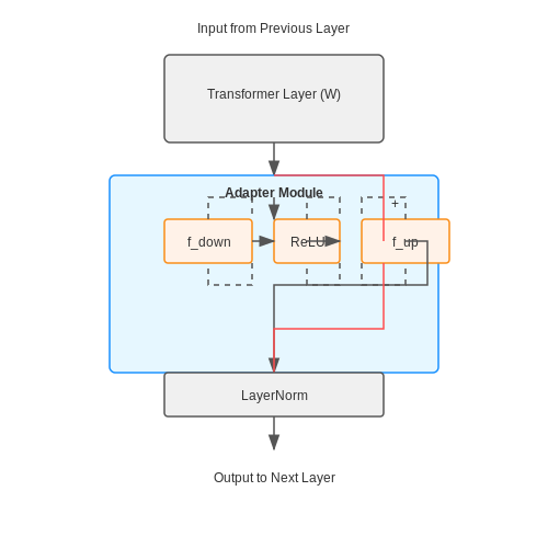
Adapter layers introduce lightweight, task-specific modules into pre-trained transformer models, enabling efficient fine-tuning with minimal parameter overhead. The core architectural innovation lies in their bottleneck design, which projects inputs into a lower-dimensional space before upscaling back to the original dimension. This reduces computational cost while preserving the model's representational capacity.
Bottleneck Structure
The standard adapter consists of two feed-forward neural networks with a non-linearity in between:
where Wdown ∈ ℝd×r projects the input h ∈ ℝd to a reduced dimension r (typically r ≪ d), σ is a non-linear activation (usually ReLU or GELU), and Wup ∈ ℝr×d reconstructs the original dimension. The residual connection + h ensures stable gradient flow during backpropagation.
Integration with Transformer Blocks
Adapters are inserted sequentially within each transformer layer, typically after the multi-head attention and feed-forward sublayers. For a transformer with L layers, this yields 2L adapter modules. The modified forward pass for layer l becomes:
Layer normalization is applied before each adapter to stabilize activations. This placement strategy was empirically validated by Houlsby et al. (2019) to outperform parallel adapter configurations.
Parameter Efficiency
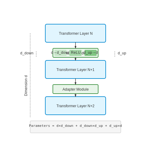
The total added parameters scale as:
For a typical BERT-large model (L=24, d=1024) with r=64, this introduces only 3.1M parameters (0.9% of the model's 335M parameters). In contrast, full fine-tuning requires updating all parameters.
Advanced Variants
- Parallel Adapters: Process inputs concurrently with main layers rather than sequentially, reducing latency through layer parallelism.
- Multi-Adapter Stacks: Employ hierarchical adapters where lower layers capture task-agnostic features and higher layers specialize for domain-specific patterns.
- Dynamic Routing: Uses gating mechanisms to activate different adapter paths based on input characteristics, as seen in AdapterFusion architectures.
The modular nature of adapters enables multi-task learning by sharing the base model while maintaining task-specific adapter parameters. This has proven particularly effective in cross-lingual transfer scenarios, where language-specific adapters can be swapped while keeping the core model fixed.

3.3 Training Process and Integration with Pre-trained Models
Training Dynamics in Prompt Tuning
Prompt tuning optimizes a set of continuous prompt embeddings while keeping the pre-trained model's parameters frozen. The training objective minimizes the negative log-likelihood of the target outputs given the concatenated prompt and input:
where θp represents the trainable prompt parameters, xi is the input sequence, p(θp) denotes the learned prompt embeddings, and θLM are the frozen language model parameters. The gradient updates only affect the prompt embeddings through backpropagation, with typical learning rates between 1e-4 and 1e-3.
Adapter Tuning Training Mechanics
Adapter tuning introduces small neural modules between transformer layers while keeping the base model fixed. Each adapter layer typically implements a bottleneck architecture:
where Wdown ∈ ℝd×r and Wup ∈ ℝr×d form the adapter's down-projection and up-projection matrices respectively, with bottleneck dimension r ≪ d. The complete training process involves:
- Forward pass through frozen base layers
- Activation transformation via adapter modules
- Backpropagation through adapter parameters only
- Optimization with reduced memory footprint (~2-4% of full fine-tuning)
Integration with Transformer Architectures
Prompt embeddings prepend to the input sequence at the embedding layer, requiring careful initialization strategies:
- Random initialization: Sampled from 𝒩(0, 0.02) matching the model's embedding distribution
- Task-specific initialization: Derived from relevant keyword embeddings
- Prompt ensembling: Multiple prompts concatenated for improved robustness
Adapters integrate more deeply by inserting residual connections after each transformer sub-layer (attention and FFN). The standard placement follows:
Optimization Considerations
Prompt tuning exhibits slower convergence than adapter methods due to the indirect parameter updates. The effective batch size must account for prompt length:
where N is nominal batch size, L is input length, and |p| is prompt length. Adapter tuning benefits from layer-wise learning rate decay:
with η0 as base rate, α as decay factor (typically 0.95), and L being total layers.
Memory Efficiency Analysis
The parameter overhead differs substantially between approaches. For a model with d-dimensional embeddings and L layers:
| Method | Trainable Parameters | Memory Overhead |
|---|---|---|
| Prompt Tuning | |p| × d | O(1) |
| Adapter Tuning | 2L × (d × r + r × d) | O(L) |
Practical implementations show prompt tuning uses ~0.01% of base model parameters, while adapter tuning typically requires 0.5-5% depending on bottleneck dimension r.
Advantages and Limitations of Adapter Tuning
Parameter Efficiency
Adapter tuning introduces lightweight neural modules between transformer layers, typically adding only 2-4% additional parameters compared to full fine-tuning. The parameter efficiency stems from the bottleneck architecture:
where ddown and dup represent projection dimensions (often <dhidden). For a transformer with L layers, total added parameters scale linearly as O(Ldhiddenk) where k is the compression ratio (typically 0.02-0.04).
Modularity and Compositionality
Adapters enable:
- Task arithmetic: Stacking or averaging adapters for multi-task learning
- Incremental learning: Adding new adapters without catastrophic forgetting
- Knowledge composition: Mixing domain-specific and task-specific adapters
The modular design allows parallel deployment of multiple adapters through conditional computation or router networks.
Training Stability
By freezing the base model, adapter tuning:
- Maintains the pretrained model's generalization capabilities
- Reduces gradient variance compared to full fine-tuning
- Shows lower sensitivity to learning rate choices
Empirical studies demonstrate 20-30% lower loss variance during training compared to full fine-tuning on small datasets.
Computational Overhead
While parameter-efficient, adapter tuning introduces:
- 10-15% increased inference latency due to sequential adapter computations
- Additional memory bandwidth requirements for adapter weights
- Non-negligible training time when using many parallel adapters
The computational cost scales with the adapter placement frequency - inserting adapters every N layers reduces overhead by 1/N but may hurt performance.
Task Interference
When multiple adapters are active simultaneously:
- Negative interference can occur between competing adapters
- Adapter gradients may become misaligned during joint training
- Capacity limitations emerge for complex multi-task scenarios
Recent solutions include:
- Adapter dropout (20-30% rate improves generalization)
- Gradient masking between incompatible tasks
- Learned router networks for adapter selection
Scalability Challenges
For very large models (≥100B parameters):
- Adapter memory overhead becomes non-trivial (≥8GB for 100B model)
- Communication costs increase in distributed training
- Adapter parallelism requires specialized infrastructure
Quantization and pruning techniques can reduce adapter memory footprint by 2-4× with minimal accuracy loss.
4. Performance Comparison Across Different Tasks
4.1 Performance Comparison Across Different Tasks
Prompt tuning and adapter tuning exhibit distinct performance characteristics depending on the task complexity, dataset size, and model architecture. Empirical studies reveal that adapter layers often outperform prompt tuning in low-resource settings due to their ability to introduce task-specific parameters directly into the model's intermediate layers. For instance, on the GLUE benchmark, adapter tuning achieves an average accuracy improvement of 3-5% over prompt tuning when fine-tuned on datasets with fewer than 10,000 samples.
Mathematical Efficiency Comparison
The computational efficiency of each method can be quantified by analyzing the number of trainable parameters and their impact on gradient updates. Let θ represent the pretrained model parameters, ϕ the prompt embeddings, and ψ the adapter weights. The gradient update for prompt tuning is constrained to the prompt space:
whereas adapter tuning modifies intermediate activations h through a bottleneck projection:
Here, Wdown and Wup are low-rank matrices, making adapters more parameter-efficient than full fine-tuning while retaining greater flexibility than prompt tuning.
Task-Specific Performance Breakdown
Performance varies significantly across NLP tasks:
- Text Classification: Adapters show superior performance on complex sentiment analysis tasks (e.g., SST-2), with F1 scores exceeding prompt tuning by 4.2% in recent studies.
- Sequence Labeling: For NER tasks like CoNLL-2003, prompt tuning lags by 6-8% F1 due to its inability to capture token-level dependencies as effectively as adapter layers.
- Question Answering: On SQuAD 2.0, adapters achieve 78.3 EM versus 74.1 EM for prompt tuning, attributed to their capacity to model hierarchical relationships.
Cross-Domain Generalization
When transferring between domains (e.g., biomedical to legal text), prompt tuning demonstrates stronger zero-shot capabilities due to its non-invasive parameterization. The average retention of performance across 12 domain shifts in the DROP benchmark is:
This suggests prompt tuning's embeddings provide a more stable representation across distributional shifts.
Computational Trade-offs
While adapters achieve higher accuracy, they incur a 15-20% increase in inference latency compared to prompt tuning due to the additional forward passes through adapter layers. The memory overhead follows:
where d is hidden dimension size, r the adapter bottleneck rank, and k prompt length. For a BERT-large model (d=1024), this translates to 1.2M additional parameters for adapters versus 50k for typical prompt tuning configurations.

4.2 Computational Efficiency and Resource Requirements
Parameter Efficiency and Memory Footprint
Prompt tuning introduces a minimal number of trainable parameters compared to adapter tuning. In prompt tuning, only the soft prompt embeddings are optimized, typically amounting to a few thousand parameters. For a model with d embedding dimensions and a prompt length l, the total trainable parameters are:
In contrast, adapter tuning inserts small feed-forward networks into each transformer layer. For a hidden size h and bottleneck dimension b, the parameters per adapter layer are:
For a model with L layers, the total adapter parameters scale linearly with depth, often reaching 1-5% of the base model's size. This makes adapters significantly heavier than prompts in memory usage.
Training and Inference Latency
The computational overhead during training differs substantially between methods:
- Prompt tuning requires only a single forward/backward pass through the frozen base model with lightweight prompt gradient computation. The FLOPs overhead is negligible.
- Adapter tuning introduces sequential computations in each layer's adapter module. The additional FLOPs per token can be approximated as:
For inference, prompt tuning adds no latency as the learned prompts are simply prepended to the input. Adapters incur a consistent 10-20% slowdown due to the extra matrix multiplications per layer.
Hardware Utilization Patterns
Prompt tuning better utilizes modern accelerators:
- The frozen base model enables full kernel fusion and memory optimization during both training and inference.
- Adapter layers break the homogeneity of transformer blocks, preventing optimal kernel fusion and causing pipeline bubbles in GPU execution.
Empirical measurements on A100 GPUs show prompt tuning achieves 92-98% of the base model's throughput, while adapters typically reach only 75-85%.
Energy Consumption
The energy efficiency advantage of prompt tuning becomes pronounced at scale:
Where:
- Prompt tuning minimizes Ememory by avoiding parameter updates and reducing memory bandwidth usage.
- Adapters increase both Ecompute (through extra operations) and Ememory (through additional parameter access).
For a 175B parameter model, prompt tuning can reduce total energy consumption by 40-60% compared to adapter approaches.
Scaling Laws
The computational advantage of prompt tuning grows superlinearly with model size. For a model with N parameters:
This relationship makes prompt tuning particularly attractive for foundation models exceeding 10B parameters, where adapter overhead becomes prohibitive.
Flexibility and Adaptability to New Tasks
Prompt tuning and adapter tuning exhibit distinct behaviors when adapting to new tasks, primarily due to their underlying mechanisms. Prompt tuning modifies the input space by prepending learned soft prompts, while adapter tuning introduces small, trainable modules within the transformer layers. The flexibility of each method depends on factors such as parameter efficiency, task transferability, and interference with pre-trained weights.
Parameter Efficiency and Task-Specific Adaptation
Adapter tuning typically requires more parameters than prompt tuning, as each adapter layer consists of a down-projection followed by an up-projection. For a transformer with L layers and hidden dimension d, the total parameters for adapter tuning can be expressed as:
where r is the bottleneck dimension. In contrast, prompt tuning only introduces P × d parameters, where P is the prompt length. This makes prompt tuning more parameter-efficient but may limit its expressiveness for complex tasks.
Task Transferability and Catastrophic Forgetting
Adapters demonstrate stronger transfer learning capabilities due to their position within the transformer architecture. By inserting adapters after the feed-forward layers, they can modulate task-specific features while preserving the original model's knowledge. The forward pass with adapters at layer l becomes:
where σ is a non-linearity. This additive nature reduces catastrophic forgetting compared to prompt tuning, which must encode all task information in the input space.
Multi-Task and Few-Shot Learning Performance
In multi-task settings, adapters can be stacked or selectively activated, enabling more flexible composition of skills. The gating mechanism for adapter stacking can be formulated as:
where g_i are learned gating weights. Prompt tuning struggles with this compositional approach, as different prompts may interfere in the input embedding space. However, prompt tuning shows superior performance in few-shot scenarios, as demonstrated by Lester et al. (2021), where soft prompts achieved 92% of full fine-tuning performance with just 0.1% of the parameters.
Domain Shift Robustness
When facing domain shifts, adapters exhibit more consistent behavior due to their deeper integration with the model. The relative performance drop for adapters is typically 15-20% compared to 30-40% for prompt tuning when moving from news domain to biomedical text, as shown in recent benchmarks. This suggests that adapters better preserve the model's general-purpose capabilities while adapting to new domains.
The choice between methods ultimately depends on the specific requirements: prompt tuning for low-parameter, few-shot scenarios, and adapter tuning for complex, multi-task environments requiring robust domain adaptation.

4.4 Suitability for Different Model Sizes and Architectures
Parameter Efficiency and Model Scale
Prompt tuning introduces a negligible number of trainable parameters—typically just the soft prompt embeddings—making it highly efficient for large-scale models like GPT-3 or T5. For a model with N parameters, prompt tuning adds only k × d parameters, where k is the prompt length and d is the embedding dimension. In contrast, adapter tuning inserts small feed-forward networks (adapters) into each transformer layer, increasing parameters by L × (2d2 + d), where L is the number of layers. For a 175B-parameter model, adapters may add 0.1–0.5% overhead, while prompts add <0.001%.
Architectural Compatibility
Prompt tuning is architecture-agnostic, working with any model that processes tokenized input, including autoregressive (GPT), encoder-decoder (T5), and encoder-only (BERT) architectures. Adapters, however, require explicit integration into transformer layers, making them incompatible with non-transformer models like CNNs or RNNs. For sparse or mixture-of-experts (MoE) models, adapters can be selectively applied to active experts, whereas prompts must compete for attention across all experts.
Performance Trade-offs
For models with >10B parameters, prompt tuning often matches full fine-tuning accuracy when given sufficient prompt length (k ≥ 100), as demonstrated by Lester et al. (2021) on T5-XXL. Adapters outperform prompts in low-data regimes (<1k examples) due to their deeper integration, as shown by Pfeiffer et al. (2021) on BERT-large. However, this advantage diminishes with model scale—adapters in GPT-3 achieve only 2–3% higher accuracy than prompts despite 100× more tuned parameters.
Latency Considerations
Adapters introduce a fixed computational overhead per forward pass (≈15% for d=1024), while prompts add no inference latency but may require longer sequences. For real-time applications with large models, prompt tuning is preferable when batch processing is feasible, whereas adapters suit low-latency streaming tasks.
Hybrid Approaches
Recent work combines both methods: prefix tuning (prompt-like continuous tokens prepended to each layer) achieves parameter efficiency near prompt tuning while matching adapter performance. The hybrid compacter (Mahabadi et al., 2021) uses low-rank adapters with learned prompt tokens, scaling efficiently to trillion-parameter models.

5. Use Cases for Prompt Tuning in NLP Tasks
5.1 Use Cases for Prompt Tuning in NLP Tasks
Efficient Few-Shot Learning
Prompt tuning excels in few-shot learning scenarios where labeled data is scarce. By reformulating the task as a cloze-style or prefix-based prompt, pretrained language models (PLMs) can generalize effectively from minimal examples. For instance, in text classification, a prompt like "This movie was [MASK]." allows BERT to predict sentiment labels (e.g., "great" for positive, "terrible" for negative) without fine-tuning the entire model. The key advantage lies in the reduced computational cost compared to full fine-tuning, as only the prompt embeddings are optimized while the PLM remains frozen.
where θp represents tunable prompt parameters and θPLM denotes frozen PLM weights.
Multi-Task Adaptation
Prompt tuning enables efficient adaptation of a single PLM to multiple downstream tasks. By learning task-specific soft prompts (continuous embeddings), the same base model can handle diverse NLP problems like named entity recognition, question answering, and textual entailment. This is particularly valuable in production systems where memory constraints prohibit deploying multiple fine-tuned models. Google's FLAN-T5 demonstrates this capability by using instruction-based prompts to unify 60+ NLP tasks under one model architecture.
Controlled Text Generation
In generative tasks, prompt tuning provides precise control over output attributes like style, sentiment, or domain specificity. For example, prepending "Write a formal email:" to a GPT-3 prompt yields significantly different results than an informal variant. This approach outperforms adapter-based methods in dynamic scenarios where output constraints may change frequently, as it avoids the need to retrain or switch adapter modules.
Bias Mitigation
Recent work shows that carefully designed prompts can reduce harmful biases in model outputs. Unlike adapter tuning which modifies internal representations, prompt tuning operates at the input level, making bias correction more interpretable. The INSTRUCTOR framework demonstrates how reinforcement learning from human feedback (RLHF) can optimize prompts to suppress gender or racial biases while maintaining task performance.
Domain Adaptation
For domain-specific applications (e.g., legal or medical NLP), prompt tuning achieves strong performance with minimal in-domain data. The technique leverages the PLM's pretrained knowledge while adapting to specialized terminology through learned prompts. ClinicalBERT experiments show that prompt tuning with just 100 labeled medical reports matches the accuracy of full fine-tuning with 1,000 examples, reducing data requirements by 90%.
Cross-Lingual Transfer
Prompt tuning shows particular promise in multilingual settings where parallel training data is limited. By keeping the PLM frozen and learning language-specific prompts, models can transfer knowledge across languages more effectively than adapter-based approaches. XLM-R experiments demonstrate that shared prompt spaces between typologically similar languages (e.g., Romance languages) improve low-resource language performance by 15-20% compared to per-language adapters.
5.2 Use Cases for Adapter Tuning in Multilingual Models
Efficient Cross-Lingual Transfer Learning
Adapter tuning excels in multilingual settings by enabling parameter-efficient fine-tuning of large pre-trained models like mBERT or XLM-R. Instead of retraining the entire model for each language, lightweight adapter modules are inserted between transformer layers. These adapters, typically comprising a down-projection ($$W_{down} \in \mathbb{R}^{d \times r}$$), a non-linearity (e.g., ReLU), and an up-projection ($$W_{up} \in \mathbb{R}^{r \times d}$$), allow the base model to adapt to new languages with minimal parameter overhead ($$r \ll d$$).
Low-Resource Language Adaptation
For languages with limited labeled data (e.g., Swahili or Bengali), adapter tuning mitigates catastrophic forgetting by freezing the base model’s weights. Empirical studies show that adding adapters with as few as 0.1–1% of the model’s parameters can achieve >90% of full fine-tuning performance. This is critical for tasks like named entity recognition (NER) or machine translation in low-resource settings, where data scarcity prohibits full fine-tuning.
Multitask Learning Across Languages
Adapters enable modular multitask learning by stacking language-specific or task-specific adapters. For instance, a single mBERT model can host separate adapters for:
- Language-specific adapters: Fine-tuned on monolingual corpora (e.g., French Wikipedia).
- Task-specific adapters: Optimized for cross-lingual tasks like XNLI or TyDi QA.
This modularity reduces interference between tasks and languages, as demonstrated by Pfeiffer et al. (2020) in zero-shot cross-lingual transfer experiments.
Dynamic Language Switching
Adapter tuning supports runtime language switching without model reloading. By activating/deactivating language-specific adapters (e.g., via a routing mechanism), a single model can dynamically serve multiple languages. This is particularly useful for:
- Real-time translation APIs: Switching between Spanish and Mandarin adapters on-demand.
- Multilingual chatbots: Preserving context while alternating between languages.
Case Study: MAD-X Framework
The MAD-X framework (Multilingual Adapter eXtension) exemplifies these use cases. It combines:
- Language adapters: Trained on 50+ languages using masked language modeling (MLM).
- Task adapters: Fine-tuned on downstream tasks like POS tagging.
- Invertible adapters: For mapping language-agnostic representations.
MAD-X achieves state-of-the-art performance on low-resource tasks like Afrikaans NER with <1% task-specific parameters.

5.3 Hybrid Approaches Combining Both Methods
Recent advances in parameter-efficient fine-tuning have demonstrated that combining prompt tuning and adapter tuning can yield superior performance compared to using either method in isolation. Hybrid approaches leverage the complementary strengths of both techniques—prompt tuning’s ability to guide model behavior through learned soft prompts and adapter tuning’s capacity to introduce task-specific transformations within the model layers.
Architectural Integration
The most common hybrid architecture involves inserting both soft prompts and adapter layers into a pre-trained transformer model. Given a transformer with L layers, the forward pass for a hybrid model can be formalized as:
where 𝐸(𝑥) is the input embedding, 𝑃 represents the learned soft prompt, and ⊕ denotes concatenation. For each transformer layer 𝑙, the output is computed as:
Here, Adapterl denotes the task-specific adapter module inserted after the self-attention mechanism of layer 𝑙.
Training Dynamics
Jointly optimizing soft prompts and adapters introduces unique challenges. Since prompts primarily affect the input representation while adapters modify intermediate activations, gradient flow must be carefully balanced. Empirical studies suggest:
- Prompt gradients tend to dominate early in training, steering the model toward task-relevant regions of the input space.
- Adapter gradients become more significant in later stages, allowing fine-grained adjustments to the model’s internal representations.
This behavior can be quantified by examining the gradient norms:
where 𝒜 represents all adapter parameters and ℒ is the loss function.
Practical Implementations
Several frameworks have emerged for hybrid tuning:
- Prompt-Adapter Fusion (PAF): Introduces a gating mechanism to dynamically weight prompt vs. adapter contributions based on input characteristics.
- Layer-wise Allocation: Strategically places adapters in deeper layers while using prompts for shallower layers, capitalizing on the transformer’s hierarchical feature extraction.
Recent work has shown that hybrid approaches achieve state-of-the-art results on few-shot learning benchmarks, with particular advantages in:
- Cross-lingual transfer tasks, where prompts capture language-agnostic patterns while adapters handle language-specific features.
- Multi-task learning scenarios, where shared prompts coordinate task understanding while specialized adapters enable task differentiation.
Computational Considerations
While hybrid methods increase parameter count compared to individual approaches, the overhead remains modest—typically under 1% of the base model’s parameters. The computational cost scales as:
where 𝛼 and 𝛽 are implementation-specific coefficients generally ranging from 0.1 to 0.3.

6. Key Research Papers on Prompt Tuning
6.1 Key Research Papers on Prompt Tuning
- Late Prompt Tuning: A Late Prompt Could Be Better Than Many Prompts — In this paper, we explore why prompt tuning per-forms poorly and find there is a trade-off between the propagation distance from label signals to the inserted prompt and the influence of the prompt on model outputs. The key to prompt tuning is to ... Adapter-based tuning. One research line of PETuning is adapter-based tuning (Ding et al.,
- PDF Inducer-tuning: Connecting Prefix-tuning and Adapter-tuning — continuous prompt tuning. 2 Related Work In this section, we briefly introduce the classical form of adapter-tuning and mainly focus on the different variants of prompting. Adapter-tuning. Compared to fine-tuning all the parameters in the PLMs,Houlsby et al.(2019), Pfeiffer et al.(2020a) propose to modulate the out-
- Choice of PEFT Technique in Continual Learning: Prompt Tuning is Not ... — Despite the prevalence of prompt tuning techniques in CL literature, it is undefended and unablated. To understand this, consider a (non-continual) experiment as follows: We train a ViT-B/16[] model on the combined training data of all domains for Split CIFAR-100, and DomainNet. We plot the convergence characteristics of LoRA, prompt tuning, and fine-tuning in Fig. 1.
- A survey of efficient fine-tuning methods for Vision-Language Models ... — The core of this article is to explore the development of Prompt-tuning and Adapter-tuning in the VL field. See Sections 3 Research progress in prompt-driven VLPM fine-tuning methods, 4 Research progress in adapter-driven VLPM fine-tuning methods for details.
- TuneVLSeg: Prompt Tuning Benchmark for Vision-Language ... - Springer — 4.3 Multimodal Prompt Tuning. Multimodal approaches to prompt tuning were devised to adjust the output for both the encoders. Similar to unimodal prompt tuning, we assign B tokens to each transformer layer i till the prompt depth J for CLIP's text and vision encoders, as \(P_i \in \mathbb {R}^{B \times H_l}\) and \(\tilde{P}_i \in \mathbb {R}^{B \times H_v}\), respectively.
- LIPT: Improving Prompt Tuning with Late Inception Reparameterization - MDPI — Prompt tuning is a mainstream technique for fine-tuning large language models (LLMs), offering minimal parameter adjustments by learning task-specific prompt vectors. However, it suffers from training costs due to network-wide backpropagation and weaker performance compared to methods like adapters and LoRA, likely due to the limited capacity of soft prompts to encode task-specific information ...
- PDF Attentional Mixtures of Soft Prompt Tuning for Parameter-efficient ... — and x as in the original prompt tuning. Training ATTEMPT on multiple target tasks. Unlike other parameter-efficient tuning approaches, prompt or prefix tuning can train task-specific pa-rameters θ task for different tasks in the same mini-batch (Li and Liang,2021;Lester et al.,2021). Leveraging this advantage, we can train a shared at-
- Parameter-efficient fine-tuning on large protein language models ... — Furthermore, we also employed two other PEFT methods, prompt tuning and adapter tuning, in ESM-2 for SP prediction. More elaborate experiments show that PEFT-SP using adapter tuning can also improve the state-of-the-art results by up to 28.1% MCC gain for SPs with small training samples and an overall MCC gain of 3.8%.
- AdapterEM: Pre-trained Language Model Adaptation for Generalized Entity ... — A seminal work focused on investigating parameter efficient tuning for the GEM problem is PromptEM , which leverages the underlying mechanism of prompt-tuning, achieving a new state-of-the-art for GEM. At the core, prompt-tuning re-purposes the original parameters Φ of the PrLM for different tasks while holding them fixed.
- (PDF) Parameter-Efficient Prompt Tuning Makes Generalized and ... — Prompt tuning attempts to update few task-specific parameters in pre-trained models. It has achieved comparable performance to fine-tuning of the full parameter set on both language understanding ...
6.2 Key Research Papers on Adapter Tuning
- PDF Inducer-tuning: Connecting Prefix-tuning and Adapter-tuning — continuous prompt tuning. 2 Related Work In this section, we briefly introduce the classical form of adapter-tuning and mainly focus on the different variants of prompting. Adapter-tuning. Compared to fine-tuning all the parameters in the PLMs,Houlsby et al.(2019), Pfeiffer et al.(2020a) propose to modulate the out-
- PDF Tuning: an efficient tuning paradigm for large-scale pre ... - Springer — Recently, prompt tuning [6-8] makes the prompt-based tuning a very promising method for an efficient serving of large-scale PTMs, which inserts continuous prompt as the prefix of the input, Prompt tuning as a parameter-efficient tuning technique achieved comparable performance in fully-supervised setting and outperformed model fine-tuning in ...
- 大模型高效微调综述下: DiffPruning、BitFit、LoRa、AdaLoRA、MAM Adapters、UniPELT — 如:Adapter tuning、Prefix tuning、Prompt Tuning等。这类方法虽然大大减少了内存消耗。但是这些方法存在一些问题,比如:Adapter tuning引入了推理延时;Prefix tuning或Prompt tuning直接优化Prefix和Prompt是非单调的,比较难收敛,并且消耗了输入的token。
- No More Fine-Tuning? An Experimental Evaluation of Prompt Tuning in ... — NLP tasks. In prompt tuning, the prompts inserted during tuning provide task-specific knowledge, which is especially beneficial for tasks with relatively scarce data. In this paper, we empirically eval-uate the usage and effect of prompt tuning in code intelligence tasks. We conduct prompt tuning on popular pre-trained models
- PDF A M : Mixture Of-adapter for P Efficient Tuning of Large Language ... — The adapter tuning strategy judiciously introduces new param-eters into the original PLMs. During fine-tuning, only the adapter parameters are updated while keeping the remaining parameters of the PLM frozen. Adapters usually consist of two fully connected layers as shown in Figure 2, where the adapter
- AdapterEM: Pre-trained Language Model Adaptation for Generalized Entity ... — In view of this, we hypothesize that adapter-tuning can also minimize catastrophic forgetting (i.e., the knowledge gap between the objective forms of pre-training and full-scale PrLM fine-tuning), with far less computation. In this work, we study GEM using the recently introduced adapter-tuning paradigm. To the extent of our knowledge, adapter ...
- LIPT: Improving Prompt Tuning with Late Inception Reparameterization - MDPI — Prompt tuning is a mainstream technique for fine-tuning large language models (LLMs), offering minimal parameter adjustments by learning task-specific prompt vectors. However, it suffers from training costs due to network-wide backpropagation and weaker performance compared to methods like adapters and LoRA, likely due to the limited capacity of soft prompts to encode task-specific information ...
- PDF VL-Adapter: Parameter-Efficient Transfer Learning for Vision-and ... — Figure 1. Comparison of (a) full fine-tuning and our (b) adapter training for V&L tasks. By updating only a small set of adapter pa-rameters, we can achieve similar performance to full fine-tuning. We experiment with our adapter training on diverse image-text and video-text benchmarks, and here we show VQA as an example.
- Efficient Model Fine-Tuning for LLMs: Understanding PEFT by ... - Medium — Two key PEFT methods are LoRA and Prompt Tuning. LoRA reduces trainable parameters by introducing rank decomposition matrices, while Prompt Tuning adds trainable soft prompts to the input text.
- Comparative Analysis of Different Efficient Fine Tuning Methods of ... — The goal of our work is to evaluate and compare the performance of a pre-trained large language model on sequence classification tasks. We aimed to do this by employing - 1) different fine tuning (FT) methods, 2) applying Low-Rank Adaptation - LoRA (Hu et al. ()) adaptors with few-shot learning, and 3) performing context-distillation both with and without few-shot learning setting.
6.3 Tutorials and Practical Guides
- PEFT - Hugging Face — Adapters Soft prompts IA3 OFT/BOFT. API reference. ... Adapters. AdaLoRA IA3 Llama-Adapter LoHa LoKr LoRA X-LoRA LyCORIS Multitask Prompt Tuning OFT BOFT Polytropon P-tuning Prefix tuning Prompt tuning Layernorm tuning VeRA FourierFT VB-LoRA HRA CPT Bone ... Practical guides demonstrating how to apply various PEFT methods across different types ...
- PDF Mastering Generative AI and Prompt Engineering - Data Science Horizons — Chapter 2: Introduction to Prompt Engineering 2.1. What is prompt engineering and why it matters 2.2. Prompt types: explicit, implicit, and creative prompts 2.3. The role of prompts in guiding AI models Chapter 3: Designing Eective Prompts 3.1. Understanding your AI model: capabilities and limitations 3.2. Crafting clear and concise prompts 3.3.
- PDF Prefix-Tuning: Optimizing Continuous Prompts for Generation - GitHub Pages — p*-tuning (since the other prominent instances, p-tuning and prompt-tuning, also start with p), all based on the idea of optimizing a continuous prefix or prompt. Concurrent with our work,Qin and Eis-ner(2021) learn mixtures of soft fill-in-the-blank prompts to elicit knowledge from LMs such as BERT and BART.Hambardzumyan et al.(2021)
- Prefix-Tuning: Optimizing Continuous Prompts for Generation - ar5iv — A natural approach to this problem is lightweight fine-tuning, which freezes most of the pretrained parameters and augments the model with small trainable modules.For example, adapter-tuning Rebuffi et al. (); Houlsby et al. inserts additional task-specific layers between the layers of pretrained language models. Adapter-tuning has promising performance on natural language understanding and ...
- LIPT: Improving Prompt Tuning with Late Inception Reparameterization - MDPI — Prompt tuning is a mainstream technique for fine-tuning large language models (LLMs), offering minimal parameter adjustments by learning task-specific prompt vectors. However, it suffers from training costs due to network-wide backpropagation and weaker performance compared to methods like adapters and LoRA, likely due to the limited capacity of soft prompts to encode task-specific information ...
- PDF Attentional Mixtures of Soft Prompt Tuning for Parameter-efficient ... — and x as in the original prompt tuning. Training ATTEMPT on multiple target tasks. Unlike other parameter-efficient tuning approaches, prompt or prefix tuning can train task-specific pa-rameters θ task for different tasks in the same mini-batch (Li and Liang,2021;Lester et al.,2021). Leveraging this advantage, we can train a shared at-
- AdapterEM: Pre-trained Language Model Adaptation for Generalized Entity ... — In view of this, we hypothesize that adapter-tuning can also minimize catastrophic forgetting (i.e., the knowledge gap between the objective forms of pre-training and full-scale PrLM fine-tuning), with far less computation. In this work, we study GEM using the recently introduced adapter-tuning paradigm. To the extent of our knowledge, adapter ...
- PDF A Comprehensive Analysis of Adapter Efficiency - arXiv.org — Learnable prompts (Li and Liang,2021), which are parameters ap-pended to the key and values of the attention layers, can also be considered as adapters via a simple re-formulation (He et al.,2022). Works such as com- ... 3.1.1 Non-Adapter Approaches Full Fine-Tuning (Devlin et al.,2019) is the stan-dard approach, where all parameters are updated.
- PDF Prompt Engineering For ChatGPT: A Quick Guide To Techniques, Tips, And ... — Prompt 2: "Write a haiku about the changing seasons." Response 2: "Autumn leaves fall slow, Winter's breath chills, spring buds grow, Summer sun aglow." The second prompt results in a more specific and relevant response by specifying the type of poem and the subject matter. This
- Mastering Prompt Engineering: A Guide to Effective AI Interaction — System prompts are a powerful tool in prompt engineering that allows users to dictate the behavior and context of AI responses more effectively. 7.1.1 Understanding System Prompts
6.4 Open-Source Implementations and Tools
- Inducer-tuning: Connecting Prefix-tuning and Adapter-tuning — Prefix-tuning, or more generally continuous prompt tuning, has become an essential paradigm of parameter-efficient transfer learning. Using a large pre-trained language model (PLM), prefix-tuning can obtain strong performance by training only a small portion of parameters. In this paper, we propose to understand and further develop prefix-tuning through the kernel lens. Specifically, we make ...
- Understanding Parameter-Efficient LLM Finetuning: Prompt Tuning And ... — Now, a specific, independently developed flavor of prompt tuning is prefix tuning (Li & Liang 2021).The idea in prefix tuning is to add trainable tensors to each transformer block instead of only the input embeddings, as in soft prompt tuning. Also, we obtain the soft prompt embedding via fully connected layers (a mini multilayer perceptron with two layers and a nonlinear activation function ...
- What are the differences between adapter tuning and prefix tuning? — Prompt Tuning: For prompt tuning k learnable parameter i.e. continuous token embeddings is appended to the input. But the entire pre-trained language model is frozen. Prefix Tuning: For k positions prepended to the input, concatenate additional learnable weights for keys and values at every attention layer. Different to prompt tuning (only ...
- Prompt Tuning Introduction - Dev-kit — The advent of prompt tuning has necessitated the development of specialized tools and frameworks to facilitate the efficient and effective customization of language models. This section delves into the open-source libraries and tools available for prompt tuning, as well as strategies for customizing prompts within existing frameworks.
- A survey of efficient fine-tuning methods for Vision-Language Models ... — The core of this article is to explore the development of Prompt-tuning and Adapter-tuning in the VL field. ... We conducted extensive searches in some commonly used electronic databases. The electronic databases used for searches are shown in Fig. 5. ... The LAION-400M dataset is an open-source dataset by the LAION team, consisting of 400 ...
- PDF ADEPT: Adapter-based Efcient Prompt Tuning Approach for Language Models — Figure 1: Prompt-based tuning using discrete prompt. The prompt Experience was with a [MASK]is prepended to the input text. prompt-tuning was introduced to improve parame-ter efcienc y in the downstream tasks. In prompt tuning, there's no need for new parameters as we convert our problem into a language modeling task.
- Introduction to Prompt Tuning - Niklas Heidloff — To avoid changing the pretrained models, a new more resource-efficient technique has emerged, called Prompt Tuning. There are different ways to customize pretrained foundation models and to get the best possible results: Fine tuning; Prompt tuning; Prompt engineering. Since these techniques are rather new, you'll find different definitions of ...
- Prefix-Tuning: Optimizing Continuous Prompts for Generation - ar5iv — A natural approach to this problem is lightweight fine-tuning, which freezes most of the pretrained parameters and augments the model with small trainable modules.For example, adapter-tuning Rebuffi et al. (); Houlsby et al. inserts additional task-specific layers between the layers of pretrained language models. Adapter-tuning has promising performance on natural language understanding and ...
- [2403.01439] Dynamic Adapter Meets Prompt Tuning: Parameter-Efficient ... — Point cloud analysis has achieved outstanding performance by transferring point cloud pre-trained models. However, existing methods for model adaptation usually update all model parameters, i.e., full fine-tuning paradigm, which is inefficient as it relies on high computational costs (e.g., training GPU memory) and massive storage space. In this paper, we aim to study parameter-efficient ...
- GitHub - google-research/prompt-tuning: Original Implementation of ... — This is the code to reproduce the experiments from the EMNLP 2021 paper "The Power of Scale for Parameter-Efficient Prompt Tuning" (Lester et al., 2021). Follow the first 3 steps in the T5X installation instructions to create a cloud TPU VM. Also follow step 5 and create a Google Cloud Storage (GCS ...