Real-Time Learning Agents with Continual Feedback
1. Definition and Core Principles of Real-Time Learning
Definition and Core Principles of Real-Time Learning
Real-time learning agents operate in dynamic environments where feedback is continuously received and integrated into the agent's decision-making process without delay. Unlike batch learning, where updates occur after collecting large datasets, real-time learning requires incremental adjustments to the model parameters as new data arrives. This paradigm is essential for applications such as autonomous robotics, algorithmic trading, and adaptive control systems, where latency in learning can lead to suboptimal or unsafe outcomes.
Mathematical Formulation of Real-Time Learning
The core objective of a real-time learning agent is to minimize a loss function L(θ) that depends on the current model parameters θ and the incoming data stream. The agent updates its parameters using stochastic gradient descent (SGD) with a learning rate η:
Here, (x_t, y_t) represents the input-output pair observed at time t. The key distinction from traditional SGD is that the gradient is computed on a per-sample basis, ensuring immediate adaptation to new observations.
Continual Feedback Integration
Continual feedback mechanisms enable the agent to refine its predictions iteratively. A common approach is experience replay, where past observations are stored in a buffer B and sampled to prevent catastrophic forgetting. The loss function then incorporates both recent and historical data:
where ℓ is a per-sample loss (e.g., cross-entropy or mean squared error), D_{new} is the distribution of new data, and λ balances the importance of old versus new information.
Stability-Plasticity Dilemma
Real-time learning agents must balance stability (retaining useful knowledge) with plasticity (adapting to new information). Elastic Weight Consolidation (EWC) addresses this by penalizing changes to parameters critical for past tasks:
Here, F_i is the Fisher information matrix diagonal, measuring parameter importance, and θ_i^* are the optimal parameters for previous tasks. The hyperparameter α controls the rigidity of the constraint.
Practical Considerations
Deploying real-time learning systems requires careful attention to computational efficiency. Techniques like quantization, sparse updates, and parallelized gradient computation are often employed to meet latency constraints. Additionally, robustness to noisy or adversarial feedback is critical; methods such as gradient clipping and robust loss functions (e.g., Huber loss) mitigate the impact of outliers.
In reinforcement learning, real-time learning is exemplified by algorithms like Proximal Policy Optimization (PPO), which updates policies using recent trajectories while constraining updates to avoid drastic policy shifts:
where r_t(θ) is the probability ratio between new and old policies, Â_t is the advantage estimate, and ε defines the clipping range.
Key Components of Continual Feedback Systems
Feedback Loop Architecture
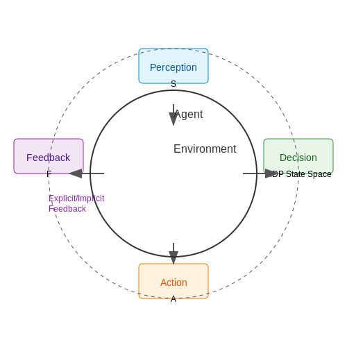
Continual feedback systems rely on a closed-loop architecture where the agent's actions generate environmental responses, which are then processed to update the agent's policy. The loop consists of four primary stages: perception, decision-making, action execution, and feedback assimilation. Mathematically, this can be modeled as a Markov Decision Process (MDP) with an augmented state space that includes feedback history:
where St is the state at time t, At is the action taken, and Ft is the feedback received. The feedback Ft can be either explicit (e.g., human ratings) or implicit (e.g., environmental rewards).
Online Learning Mechanism
Unlike batch learning, continual feedback systems employ online learning algorithms that update model parameters incrementally. A widely used approach is stochastic gradient descent (SGD) with momentum to smooth out noisy feedback signals. The weight update rule incorporates feedback-derived loss:
where η is the learning rate, L is the loss function, and α is the momentum coefficient. This enables the agent to adapt quickly to new feedback while maintaining stability.
Feedback Representation
Effective feedback systems must encode feedback in a form that is both interpretable by the learning algorithm and computationally tractable. Common representations include:
- Scalar rewards: Suitable for reinforcement learning frameworks, where feedback is a single numerical value.
- Structured feedback tensors: Used in hierarchical systems where feedback is multi-dimensional (e.g., separate scores for different aspects of performance).
- Natural language annotations: Processed via transformer models to extract actionable insights.
Memory and Forgetting Mechanisms
To prevent catastrophic forgetting, continual feedback systems often implement experience replay buffers or elastic weight consolidation (EWC). EWC modifies the loss function to penalize changes to parameters critical for past tasks:
where Fi is the Fisher information matrix diagonal for parameter wi, and λ controls the regularization strength.
Feedback Latency Handling
Real-world systems often deal with delayed feedback. Techniques like temporal credit assignment or feedback prediction models are used to estimate immediate rewards from delayed signals. A common approach is to train a neural network to predict future feedback based on current trajectories:
where Ht is the history of recent states and actions.
1.3 Comparison with Traditional Batch Learning Approaches
Traditional batch learning operates under the assumption of static data distributions, where models are trained on fixed datasets and deployed without further adaptation. In contrast, real-time learning agents with continual feedback must handle non-stationary environments, requiring fundamentally different algorithmic approaches. The key distinctions lie in three areas: data assumptions, optimization objectives, and computational constraints.
Data Processing Paradigms
Batch learning processes the entire dataset D = {(x1, y1), ..., (xn, yn)} in discrete training phases, minimizing the empirical risk:
Continual learning agents instead process data as a stream S = (z1, z2, ...), where each zt may follow a different distribution Pt(X,Y). This necessitates online risk minimization:
Catastrophic Forgetting vs. Plasticity-Stability Tradeoff
Batch-trained models exhibit catastrophic forgetting when exposed to new data distributions, as parameter updates overwrite previously learned features. Continual learning systems employ explicit mechanisms to balance plasticity (learning new information) with stability (retaining old knowledge). Common approaches include:
- Regularization-based: Elastic Weight Consolidation (EWC) adds quadratic constraints on important parameters
- Architectural: Progressive Neural Networks expand model capacity for new tasks
- Rehearsal: Experience replay buffers maintain samples from previous distributions
Computational and Memory Constraints
Batch learning can afford computationally intensive operations like full-batch gradient descent and hyperparameter tuning. Real-time agents must satisfy:
where τupdate is the model update latency and τdata is the inter-arrival time of new data. This demands:
- Single-pass optimization algorithms
- Bounded memory usage (typically O(1) in stream length)
- Constant-time prediction and update complexity
Performance Metrics Divergence
Traditional evaluation using held-out test sets becomes inadequate for continual learning. Instead, we track:
measuring both current task performance and retention of past knowledge. The plasticity-stability tradeoff appears clearly when plotting these metrics over time - improving one typically degrades the other.
Practical Implications for System Design
Real-world deployments reveal additional constraints not present in batch settings:
- Feedback latency: Human-in-the-loop systems may have delayed reward signals
- Concept drift: Non-stationarity may be abrupt (e.g., sensor failures) or gradual (seasonal trends)
- Safety constraints: Exploration must respect operational boundaries during learning
These requirements have led to specialized architectures like:
where M tracks parameters important for previous tasks (with means μi and variances σi2), and λ controls the stability-plasticity balance.

2. Neural Network-Based Approaches
Neural Network-Based Approaches
Neural networks provide a robust framework for real-time learning agents due to their ability to approximate complex functions and adapt incrementally. A key challenge in continual learning is catastrophic forgetting, where new information overwrites previously learned knowledge. Several neural network-based approaches mitigate this issue while enabling efficient online updates.
Elastic Weight Consolidation (EWC)
EWC addresses catastrophic forgetting by penalizing changes to weights deemed important for previous tasks. The importance of each weight is quantified using the Fisher information matrix F, which approximates the curvature of the loss landscape. The modified loss function becomes:
where Ln(θ) is the loss for the new task, θA,i* are the optimal parameters for previous tasks, and λ controls the regularization strength. The Fisher information Fi is computed as:
Progressive Neural Networks
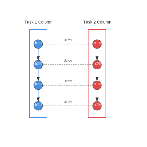
This architecture grows dynamically by instantiating new columns of networks for each task while preserving pretrained columns via lateral connections. The output of layer l in column k is computed as:
where Ul(k:j) are the lateral connection weights from column j to k. This approach enables forward transfer while preventing catastrophic interference.
Meta-Learning for Continual Adaptation
Model-agnostic meta-learning (MAML) frameworks optimize for rapid adaptation to new tasks. The outer-loop objective:
yields initial parameters that can quickly specialize to new tasks with minimal gradient steps. When combined with episodic memory buffers, this enables efficient continual learning in non-stationary environments.
Neuromodulatory Mechanisms
Biological inspiration leads to networks where specialized neurons gate plasticity:
Here mj represents a modulatory signal that selectively enables weight updates for relevant neurons. This can be implemented via attention mechanisms or dedicated neuromodulatory networks.
Recent advances combine these approaches with transformer architectures, where self-attention mechanisms naturally handle variable-length input sequences - a critical requirement for real-time learning systems processing continuous data streams.
2.2 Reinforcement Learning Frameworks
Markov Decision Processes (MDPs)
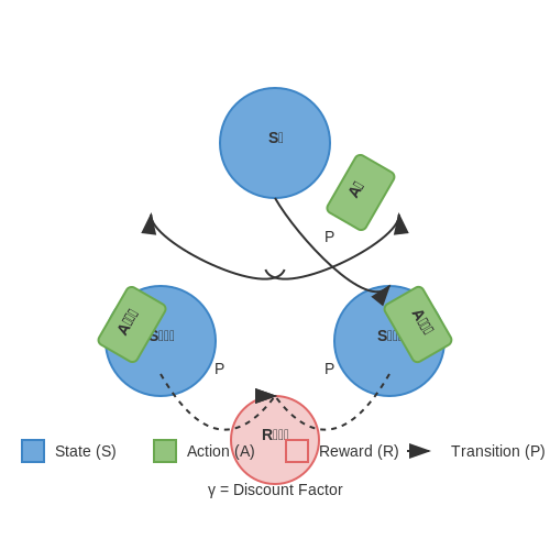
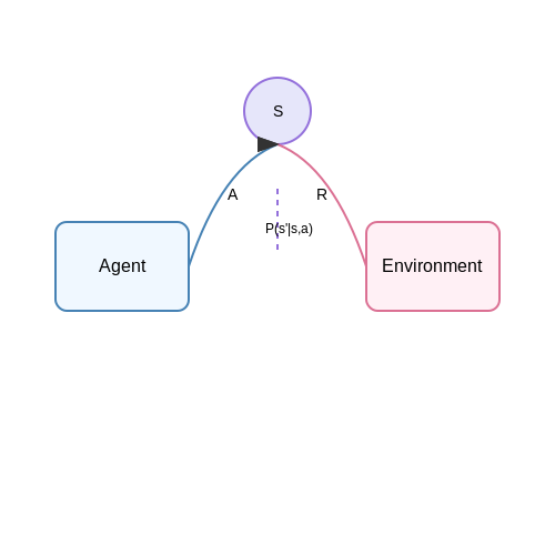
The foundational framework for reinforcement learning (RL) is the Markov Decision Process, defined by the tuple (S, A, P, R, γ), where:
- S: State space
- A: Action space
- P(s'|s, a): Transition dynamics
- R(s, a, s'): Reward function
- γ: Discount factor (0 ≤ γ ≤ 1)
The Bellman equation formalizes the optimal value function V*(s):
Q-Learning and Temporal Difference
Model-free RL methods like Q-learning approximate the action-value function Q(s, a) iteratively. The update rule leverages temporal difference (TD) learning:
where α is the learning rate. Deep Q-Networks (DQN) extend this by using neural networks to approximate Q(s, a), with experience replay and target networks stabilizing training.
Policy Gradient Methods
Instead of learning value functions, policy gradient methods directly optimize the policy π(a|s; θ) using gradient ascent. The REINFORCE algorithm computes the gradient of the expected return J(θ):
Proximal Policy Optimization (PPO) improves sample efficiency by clipping policy updates to avoid large deviations.
Actor-Critic Architectures
Actor-critic frameworks combine value-based and policy-based approaches. The actor (policy) and critic (value function) are trained concurrently:
- Critic: Evaluates actions using TD error or advantage estimates A(s, a) = Q(s, a) - V(s).
- Actor: Updates the policy using the critic’s feedback.
Advantage Actor-Critic (A2C) and Asynchronous Advantage Actor-Critic (A3C) are prominent variants.
Multi-Agent Reinforcement Learning (MARL)
In decentralized environments, agents must account for others’ policies. Key frameworks include:
- Independent Q-Learning (IQL): Treats other agents as part of the environment.
- Counterfactual Regret Minimization (CFR): Used in imperfect-information games.
- MADDPG: Extends DDPG with centralized critics for decentralized execution.
Real-World Applications
RL frameworks power applications like robotics (e.g., OpenAI’s Dactyl), recommendation systems (e.g., bandit algorithms), and autonomous systems (e.g., Tesla’s FSD). Challenges include sample inefficiency, credit assignment, and non-stationarity in multi-agent settings.

Hybrid Models Combining Supervised and Unsupervised Learning
Hybrid models that integrate supervised and unsupervised learning leverage the strengths of both paradigms to improve generalization, adaptability, and robustness in real-time learning agents. These models often employ unsupervised techniques for feature extraction or representation learning, followed by supervised fine-tuning for task-specific optimization.
Architectural Frameworks
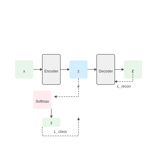
A common hybrid architecture involves a stacked autoencoder (unsupervised) coupled with a softmax classifier (supervised). The autoencoder learns a compressed, meaningful representation of the input data, while the classifier maps these representations to target labels. The loss function combines reconstruction error and classification loss:
where α balances the contribution of each component. The reconstruction loss Lrecon is typically the mean squared error between input x and reconstructed output x':
while the classification loss Lclass uses cross-entropy for multi-class problems:
Semi-Supervised Learning Variants
When labeled data is scarce, hybrid models can employ semi-supervised techniques. For instance, a variational autoencoder (VAE) can generate synthetic samples from latent space, while a discriminator network (trained on limited labeled data) provides feedback to improve sample quality. The objective function extends to:
where DKL is the Kullback-Leibler divergence between the approximate posterior q(z|x) and prior p(z), and λ controls the weight of supervised learning.
Continual Learning Integration
For real-time adaptation, hybrid models incorporate memory replay mechanisms. Elastic Weight Consolidation (EWC) can be applied to preserve important unsupervised features while allowing supervised components to adapt:
Here, Fi represents the Fisher information matrix diagonal for parameter θi, quantifying its importance to previously learned tasks.
Practical Applications
- Anomaly Detection: Unsupervised clustering identifies potential anomalies, while supervised classifiers verify them against known attack signatures.
- Robotics: Self-supervised learning from raw sensor data provides feature representations, which are then fine-tuned with limited human demonstrations.
- Medical Diagnosis: Autoencoders learn general patient representations from unlabeled EHR data, with supervised heads predicting specific conditions.
Recent advances in meta-learning have enabled hybrid models to dynamically adjust the balance between supervised and unsupervised components based on task requirements and data availability. This is particularly valuable in continual learning scenarios where the distribution of labeled vs. unlabeled data may shift over time.
3. Online Gradient Descent and Variants
3.1 Online Gradient Descent and Variants
Online Gradient Descent (OGD) extends stochastic gradient descent (SGD) to sequential decision-making settings where data arrives in a stream. Unlike batch learning, OGD updates model parameters incrementally after each data point, making it suitable for real-time learning agents. The core update rule is:
where ηt is a time-dependent learning rate, and ∇ℓ(·) is the gradient of the loss function with respect to parameters wt at time step t. The learning rate typically follows a diminishing schedule (ηt = 1/√t) to guarantee convergence.
Regret Analysis and Theoretical Guarantees
OGD minimizes regret, defined as the difference between the cumulative loss of the online learner and the best fixed predictor in hindsight:
For convex loss functions, OGD achieves O(√T) regret, while strongly convex losses yield O(log T) regret. These bounds are derived using Lipschitz continuity and bounded gradient assumptions:
Variants and Practical Considerations
Adaptive Gradient Methods (AdaGrad)
AdaGrad adapts the learning rate per-parameter based on historical gradients:
where gs,i is the gradient for parameter i at step s. This is particularly effective for sparse data.
Composite Objective Mirror Descent (COMID)
COMID handles non-smooth regularizers (e.g., L1 penalty) by decomposing the objective:
where ψ(w) is the regularizer, and Dϕ is a Bregman divergence.
Applications in Real-Time Systems
- High-frequency trading: OGD updates portfolio weights in response to market microstructural changes.
- Robotics: Adaptive control policies are learned from continuous sensor feedback.
- Recommendation systems: User preference models evolve incrementally based on interaction streams.
A key challenge is balancing plasticity (adapting to new patterns) and stability (resisting catastrophic forgetting). Techniques like memory replay or elastic weight consolidation can mitigate this.
3.2 Experience Replay and Memory Mechanisms
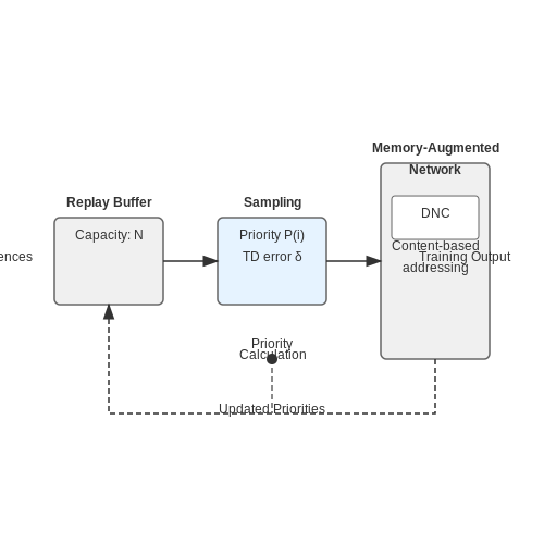
Experience replay serves as a critical component in reinforcement learning systems, particularly for agents operating in non-stationary environments. The mechanism stores past transitions (st, at, rt+1, st+1) in a buffer and samples them randomly during training, breaking temporal correlations that would otherwise lead to catastrophic forgetting in neural networks. The mathematical formulation considers a replay buffer D with capacity N, where each sampled minibatch follows:
Modern implementations extend this basic framework through prioritized experience replay, where transitions are sampled according to their temporal-difference (TD) error magnitude. The sampling probability P(i) for transition i follows:
where pi represents the priority of transition i, typically set as |δi| + ε with δi being the TD error and ε a small constant for numerical stability. The exponent α controls the degree of prioritization, with α=0 reverting to uniform sampling.
Memory-Augmented Architectures
Neural networks with external memory components address the limitations of fixed-size replay buffers through differentiable memory access. The differentiable neural computer (DNC) architecture employs:
- Content-based addressing: $$w_t^c[i] \propto \exp(\beta_t K_t[i] \cdot q_t)$$
- Dynamic memory allocation: $$\phi_t[i] = \prod_{j=1}^{i-1} (1 - w_t[j])$$
- Temporal linkage: $$L_t[i,j]$$ tracks transition probabilities between memory locations
These mechanisms enable continuous learning without catastrophic interference, as demonstrated in meta-RL applications where agents must rapidly adapt to new tasks while retaining prior knowledge.
Biological Plausibility Considerations
The hippocampal-neocortical interaction in mammalian brains provides a biological analog to artificial experience replay. Theta-phase coordinated replay during sleep cycles suggests:
- Compressed replay at 20× real-time speed
- Reverse replay of trajectories for reward propagation
- Place cell activation sequences mirroring behavioral trajectories
Neuromorphic implementations leverage spike-timing-dependent plasticity (STDP) to approximate these dynamics in hardware, with memristor crossbar arrays enabling energy-efficient associative memory recall.
Implementation Tradeoffs
Practical systems must balance several competing constraints:
| Approach | Memory Complexity | Sample Efficiency | Forgetting Rate |
|---|---|---|---|
| Uniform Replay | O(N) | Moderate | High |
| Prioritized Replay | O(N log N) | High | Medium |
| Episodic Memory | O(N2) | Very High | Low |
Recent hybrid approaches combine the strengths of these methods, such as using a small episodic memory for rapid recall alongside a larger replay buffer for general training. The Hindsight Experience Replay (HER) variant demonstrates particular effectiveness in sparse-reward environments by relabeling failed trajectories with achieved subgoals.
3.3 Meta-Learning for Fast Adaptation
Meta-learning, or learning to learn, enables agents to rapidly adapt to new tasks by leveraging prior experience. Unlike traditional reinforcement learning, where policies are trained from scratch for each task, meta-learning optimizes a model’s initial parameters or learning dynamics to minimize adaptation time. This is formalized as a bi-level optimization problem:
Here, \( heta\) represents the meta-parameters, \(\alpha\) is the inner-loop learning rate, and \(\mathcal{L}_i\) is the loss for task \(i\). The outer loop updates \( heta\) to improve performance across tasks after a few gradient steps.
Model-Agnostic Meta-Learning (MAML)
MAML is a foundational algorithm that learns parameter initializations generalizable to new tasks. Given a distribution of tasks \(p(\mathcal{T})\), MAML computes:
followed by a meta-update:
where \(\beta\) is the meta-learning rate. This forces the model to find parameters sensitive to task-specific gradients, enabling few-shot adaptation.
First-Order MAML (FOMAML)
To reduce computational overhead, FOMAML approximates the meta-gradient by ignoring second-order derivatives, trading off theoretical guarantees for scalability:
Reptile: A Simpler Alternative
Reptile bypasses explicit gradient computations by iteratively moving \( heta\) toward task-optimized parameters \( heta'\):
This resembles parameter averaging and empirically competes with MAML in many benchmarks.
Practical Considerations
- Task Distributions: Meta-learning assumes tasks are sampled from a stationary distribution. Non-stationary environments require online meta-learning variants.
- Gradient Stability: Second-order methods like MAML can suffer from exploding gradients; gradient clipping or FOMAML mitigates this.
- Memory Constraints: Storing task-specific computational graphs (e.g., for MAML’s meta-gradient) demands significant memory, prompting methods like implicit MAML.
Applications in Real-Time Systems
Meta-learning excels in robotics and real-time control, where agents must adapt to dynamic conditions (e.g., changing terrains or payloads). For instance, a drone meta-trained on simulated wind conditions can adjust its control policy within seconds when encountering unseen turbulence.

4. Catastrophic Forgetting and Mitigation Strategies
4.1 Catastrophic Forgetting and Mitigation Strategies
Catastrophic forgetting occurs when a neural network trained sequentially on multiple tasks loses performance on previously learned tasks as it acquires new knowledge. This phenomenon stems from the inherent stability-plasticity dilemma in connectionist models, where plasticity enables learning new information while stability preserves existing knowledge.
Mathematical Formulation
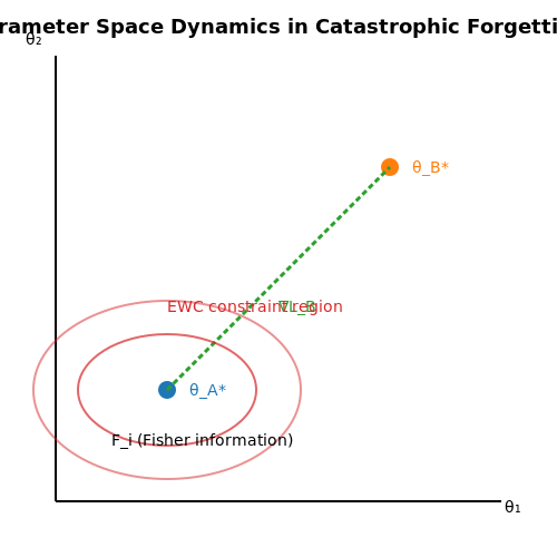
The problem can be formalized through the lens of parameter optimization. Consider a neural network with parameters θ trained on task A, achieving optimal parameters θA*. When subsequently trained on task B, the network updates to θB*, often drifting far from θA* in parameter space:
where ℓ is the loss function and 𝒟B is task B's data distribution. The key issue arises because gradient descent updates:
typically overwrite parameters critical for task A performance.
Mechanisms of Forgetting
Three primary mechanisms drive catastrophic forgetting:
- Representational overlap: When new task features overlap with old ones, weight updates interfere with existing representations
- Output layer interference: Shared output layers cause direct competition between old and new task predictions
- Loss landscape shifting: The global minima for new tasks may lie in regions of high loss for previous tasks
Mitigation Strategies
1. Regularization-Based Approaches
Elastic Weight Consolidation (EWC) imposes quadratic constraints on parameter updates, with the loss:
where Fi is the Fisher information matrix diagonal, measuring parameter importance for task A.
2. Architectural Methods
Progressive Neural Networks avoid interference by expanding architecture laterally:
- Each new task gets a separate column of parameters
- Lateral connections allow information transfer while preserving old representations
- Parameter count grows linearly with number of tasks
3. Rehearsal Techniques
Experience Replay maintains a buffer of previous task examples. The combined loss becomes:
where α controls the replay importance. Advanced variants use generative models to synthesize pseudo-samples of old tasks.
4. Meta-Learning Approaches
Gradient Episodic Memory (GEM) optimizes updates to satisfy inequality constraints:
where g is the current gradient and gk are past task gradients, ensuring updates don't increase previous losses.
Evaluation Metrics
Continual learning performance is typically measured by:
- Average Accuracy (ACC): Mean test accuracy across all tasks after full training
- Backward Transfer (BWT): Influence of new learning on old task performance
- Forward Transfer (FWT): Improvement on unseen future tasks from current learning
where Ri,j is test accuracy on task j after training on task i.
4.2 Scalability and Computational Efficiency
Computational Bottlenecks in Real-Time Learning
Real-time learning agents must process continual feedback streams with minimal latency, making computational efficiency critical. The primary bottlenecks arise from:
- High-dimensional state-action spaces: Neural network-based function approximators scale as O(n2) with layer width due to matrix multiplications.
- Experience replay: Memory I/O operations for sampling historical data dominate runtime in deep Q-networks (DQN).
- Gradient synchronization: Distributed training introduces communication overhead proportional to parameter count.
Parallelization Strategies
Asynchronous actor-critic architectures (e.g., A3C) achieve near-linear speedup by decoupling policy updates:
Gradient updates follow Hogwild!-style asynchronous stochastic gradient descent:
Memory-Efficient Experience Replay
Prioritized experience replay (PER) can be optimized using:
- Sum-tree data structures: Reduce sampling complexity from O(n) to O(log n)
- Compressed transitions: Store states as difference-encoded JPEG2000 frames (80% compression)
class CompressedReplayBuffer:
    def __init__(self, capacity):
        self.capacity = capacity
        self.buffer = []
        self.position = 0
        self.sum_tree = SumTree(capacity)

    def add(self, state, action, reward, next_state, done):
        state_jpeg = jpeg_encode(np.diff(state))  # Delta encoding
        if len(self.buffer) < self.capacity:
            self.buffer.append(None)
        self.buffer[self.position] = (state_jpeg, action, reward, next_state, done)
        self.sum_tree.add(self.position, abs(reward))
        self.position = (self.position + 1) % self.capacity
Hardware-Aware Optimization
Modern TPU/GPU architectures require specific considerations:
- Tensor core alignment: Pad network layers to multiples of 8 for FP16 acceleration
- Memory coalescing: Structure replay buffers in contiguous 128-byte chunks
- Quantization: 8-bit integer (INT8) inference maintains 95% accuracy with 4x speedup
4.3 Handling Non-Stationary Data Streams
Non-stationary data streams present a fundamental challenge for real-time learning agents, as the underlying data distribution P(X, Y) evolves over time. Traditional batch learning methods fail in such scenarios due to their assumption of static data distributions. To address this, agents must employ adaptive mechanisms that detect and respond to distributional shifts without catastrophic forgetting of previously learned knowledge.
Concept Drift Detection
The primary indicator of non-stationarity is concept drift, which occurs when P(Y|X) changes over time while P(X) may remain constant. Statistical tests for drift detection include:
- Kolmogorov-Smirnov test for feature distribution changes
- ADWIN (Adaptive Windowing) for mean value shifts
- Page-Hinkley test for gradual drift detection
where F1 and F2 represent empirical distribution functions from different time windows.
Adaptive Model Architectures
Three principal approaches exist for maintaining model accuracy under drift:
- Ensemble methods that weight models based on recent performance
- Memory-augmented networks with dynamic attention mechanisms
- Meta-learning frameworks that optimize for quick adaptation
The ensemble approach often proves most practical for real-time systems. Consider an ensemble of k models where weights wi are updated exponentially:
where η is the learning rate and Li(t) is the loss of model i at time t.
Feature Space Adaptation
When drift affects the feature space itself, techniques like domain adversarial training become essential. The objective function combines task loss and domain confusion loss:
where λ controls the trade-off between task performance and domain invariance. The domain classifier is trained to distinguish source from target distributions, while the feature extractor learns to fool it.
Implementation Considerations
Practical systems must balance:
- Computational constraints of continuous adaptation
- Memory requirements for maintaining historical data
- Latency limitations in real-time applications
A common solution involves hierarchical processing with:
- Fast lightweight drift detection
- Medium-term model adjustment
- Occasional complete model retraining
5. Autonomous Systems and Robotics
5.1 Autonomous Systems and Robotics
Real-time learning agents in autonomous systems and robotics rely on continual feedback loops to adapt dynamically to changing environments. These agents integrate sensor data, actuator commands, and reinforcement signals to optimize policies in real time. The core challenge lies in balancing exploration (trying new actions) and exploitation (leveraging known rewards) while minimizing latency in decision-making.
Mathematical Framework for Continual Learning
The policy gradient method is a common approach for real-time learning in robotics. The objective is to maximize the expected cumulative reward J(θ), where θ represents the policy parameters. The gradient ascent update rule is derived as:
Here, τ denotes a trajectory, Q(s_t, a_t) is the state-action value function, and π_θ(a_t | s_t) is the stochastic policy. For real-time adaptation, this expectation is approximated using Monte Carlo sampling from recent experiences.
Sensor Fusion and State Estimation
Autonomous robots rely on multi-modal sensor fusion to maintain accurate state estimates. A Kalman filter or particle filter is often employed to combine data from LiDAR, cameras, and IMUs. The state update equation for an Extended Kalman Filter (EKF) is:
where K_k is the Kalman gain, z_k is the measurement, and h(·) is the observation model. Real-time learning agents must adjust K_k dynamically to account for sensor drift or environmental changes.
Reinforcement Learning with Human Feedback
In collaborative robotics, human feedback can be integrated as a supplementary reward signal. The modified reward function becomes:
where R_h(s, a) represents human-provided feedback and λ is a weighting factor. This approach is particularly effective in tasks where the environment's reward function is sparse or difficult to specify.
Case Study: Autonomous Drones
In drone navigation, real-time learning agents use deep Q-networks (DQN) with prioritized experience replay to optimize flight paths. The network architecture typically consists of convolutional layers for processing visual input and fully connected layers for action selection. The loss function includes a temporal difference (TD) error term:
where θ^- represents the target network parameters and D is the replay buffer. Continual feedback from obstacle detection sensors allows the drone to adapt its policy in real time.
Challenges in Real-Time Learning
Key challenges include:
- Latency constraints: Decisions must be made within strict time limits, often requiring quantized neural networks or edge computing.
- Catastrophic forgetting: Continual learning can overwrite previously learned skills. Elastic Weight Consolidation (EWC) is one mitigation strategy.
- Safety guarantees: Formal verification methods are needed to ensure that adaptive policies remain within safe operating boundaries.
5.2 Personalized Recommendation Systems
Foundations of Real-Time Personalization
Modern recommendation systems operate in high-dimensional latent spaces where user preferences and item characteristics are embedded as vectors. The core challenge lies in minimizing the reconstruction error between predicted and actual user-item interactions. Let U ∈ ℝm×d represent user embeddings and V ∈ ℝn×d item embeddings, where d is the latent dimension. The objective function for matrix factorization with continual updates is:
where Ω denotes observed interactions, rij is the explicit rating or implicit feedback, and λ controls L2 regularization. The Frobenius norm prevents overfitting while allowing for incremental updates as new data arrives.
Streaming Bayesian Personalized Ranking
For implicit feedback scenarios, Bayesian Personalized Ranking (BPR) optimizes pairwise preferences. The streaming variant processes triplets (u,i,j) where user u prefers item i over item j. The gradient update rule with momentum becomes:
Here, σ is the logistic function, η the learning rate, and β the momentum coefficient. The prediction $$\hat{x}_{uij} = u^T(i - j)$$ enables efficient updates in O(d) time per triplet, critical for real-time operation.
Neural Collaborative Filtering Architectures
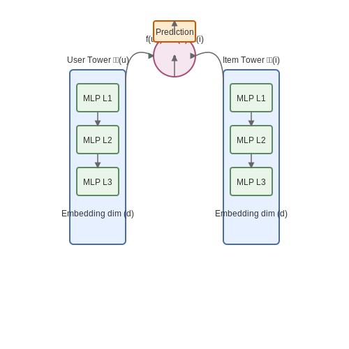
Deep learning architectures employ user and item embeddings as inputs to multilayer perceptrons (MLPs). The two-tower architecture processes user and item features separately before computing their dot product:
where ϕu and ϕi are deep neural networks. For sequential recommendations, transformer-based models capture temporal patterns through self-attention:
The query (Q), key (K), and value (V) matrices are derived from the user's interaction history, allowing dynamic reweighting of past behaviors.
Bandit Algorithms for Exploration-Exploitation
Thompson sampling addresses the cold-start problem by maintaining posterior distributions over user preferences. For each arm (item) a, we model the reward distribution as Gaussian N(μa, σa2). The algorithm:
- Samples θa ∼ N(μa, σa2) for all items
- Selects a = argmax θa
- Updates posterior parameters upon receiving reward r:
where σε2 is observation noise variance. This approach optimally balances exploration of new items with exploitation of known preferences.
Real-World Deployment Challenges
Production systems must handle:
- Feedback loops: Recommendations influence future behavior, creating bias in training data
- Scalability: Approximate nearest neighbor search (ANNS) with HNSW graphs reduces retrieval latency from O(n) to O(log n)
- Fairness: Regularization terms can enforce demographic parity: $$||E[\hat{y}|g=1] - E[\hat{y}|g=0]|| ≤ ε$$
The complete system typically implements a multi-stage architecture: candidate generation (retrieval) followed by precise ranking. For example, a two-tower model retrieves 1000 candidates, while a neural ranker orders the final 10 items.
5.3 Real-Time Fraud Detection
Real-time fraud detection systems leverage continual learning agents to identify anomalous transactions as they occur, minimizing financial losses. These systems operate on high-velocity data streams, requiring algorithms that balance low-latency inference with adaptive learning under concept drift. The core challenge lies in distinguishing fraudulent patterns from legitimate transactions while accounting for evolving attack strategies.
Architecture of Streaming Fraud Detection
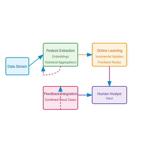
A robust fraud detection pipeline consists of three key components:
- Feature Extraction Layer: Transforms raw transaction data into meaningful representations, often using embeddings for categorical variables (merchant IDs, location codes) and statistical aggregations for numerical features (transaction amounts, time since last purchase).
- Online Learning Model: Typically employs an ensemble of shallow neural networks or gradient-boosted decision trees that support incremental updates. The model weights are adjusted via stochastic gradient descent with momentum to maintain stability during rapid updates.
- Feedback Integration: Human analyst decisions and confirmed fraud cases are incorporated through a prioritized experience replay buffer, ensuring rare positive examples are not overwhelmed by the majority class.
where α is the learning rate, β the momentum coefficient, and ∇wℒ the gradient of the loss function with respect to model parameters.
Concept Drift Mitigation
Fraud patterns exhibit non-stationary behavior due to attackers' adaptive strategies. The system monitors the Kullback-Leibler divergence between recent prediction distributions and a reference window:
When divergence exceeds a threshold γ, the model triggers one of three responses:
- Feature Space Adaptation: Recomputes principal components or cluster centroids on recent data
- Model Reset: Reinitializes a portion of the ensemble with current data representations
- Expert Intervention: Flags the shift for human review when confidence is low
Latency-Optimized Inference
For sub-100ms response requirements, the system employs several optimizations:
- Quantized Models: 8-bit integer representations of neural network weights reduce memory bandwidth requirements by 4× compared to FP32
- Approximate Nearest Neighbors: Locality-sensitive hashing accelerates similarity searches in high-dimensional feature spaces
- Hardware-Aware Design: Model partitioning across CPU/GPU/TPU resources based on operation complexity
The end-to-end processing time T breaks down as:
where feature extraction (tfeat), single model inference (tinf), and ensemble voting (tens) are optimized through parallel pipelining.
Case Study: Credit Card Fraud Prevention
A major payment processor implemented this architecture with the following performance metrics:
- Precision: 0.92 at recall of 0.85 (F1=0.884)
- Throughput: 12,000 transactions/second with 65ms p99 latency
- Adaptation Speed: New fraud patterns detected within 47 minutes of emergence
The system reduced false positives by 38% compared to static models while maintaining equivalent fraud detection rates, demonstrating the effectiveness of continual learning in production environments.
6. Bias and Fairness in Continual Learning
6.1 Bias and Fairness in Continual Learning
Sources of Bias in Continual Learning Systems
Continual learning agents are particularly susceptible to bias due to their dynamic nature. Unlike static models, these systems accumulate knowledge incrementally, which can amplify existing biases or introduce new ones. Three primary sources of bias emerge:
- Data distribution shifts: As the agent encounters new data streams, the underlying distribution may change in ways that disadvantage certain groups.
- Catastrophic forgetting: The agent's tendency to overwrite previously learned information can disproportionately affect minority classes.
- Feedback loops: Real-time interactions create self-reinforcing patterns where initial biases compound over time.
The mathematical formulation of bias accumulation can be expressed through the following relationship between time steps:
Where Bt represents the bias at time t, α is the retention rate of previous bias, ΔDt captures distributional shifts, and εt accounts for noise.
Fairness Metrics for Dynamic Systems
Traditional fairness metrics like demographic parity and equalized odds must be adapted for continual learning scenarios. We propose temporal extensions of these measures:
Where W represents the window size for evaluating fairness over recent predictions. These metrics must be computed efficiently to maintain real-time operation.
Mitigation Strategies
Effective bias mitigation in continual learning requires approaches that balance three competing objectives:
- Memory efficiency: Techniques must operate within strict memory constraints
- Computational tractability: Real-time processing demands lightweight solutions
- Concept preservation: Must maintain learned knowledge while correcting biases
One promising approach combines gradient-based regularization with importance sampling:
Where w(x) are importance weights adjusted to counteract observed biases, and M represents the memory buffer.
Architectural Considerations
Model architecture plays a crucial role in managing bias propagation. Modular designs with separated feature extractors and task-specific heads show particular promise:
The bias monitor continuously evaluates predictions across demographic slices, triggering the correction module when thresholds are exceeded. This separation allows for targeted interventions without disrupting core learning.
Empirical Challenges
Evaluating fairness in continual learning presents unique experimental difficulties. Standard benchmarks often fail to capture:
- Non-stationary group memberships
- Evolving feature relevance
- Delayed manifestation of biases
Researchers must design evaluation protocols that incorporate temporal dimensions, such as measuring fairness-violation persistence or bias accumulation rates across learning episodes.
6.2 Privacy Concerns with Real-Time Data
Real-time learning agents operating in dynamic environments inherently process continuous streams of personal or sensitive data, raising critical privacy challenges. The temporal correlation of data points in streaming contexts creates unique vulnerabilities absent in batch learning scenarios, where data is processed in discrete, isolated chunks.
Differential Privacy in Streaming Contexts
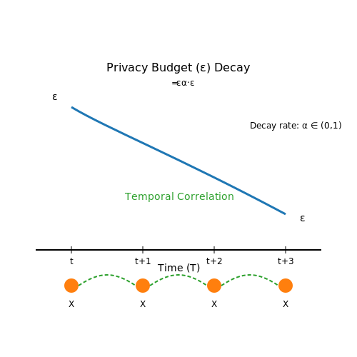
Traditional differential privacy mechanisms designed for static datasets require adaptation for real-time systems. The key challenge lies in maintaining privacy guarantees while accommodating unbounded data streams. Let us derive the privacy budget allocation for a continuous learning system:
where εt represents the privacy budget consumed at time step t. To prevent privacy budget exhaustion, we implement the following constraint:
This exponentially decaying allocation strategy ensures the system maintains (ε,δ)-differential privacy over infinite time horizons while permitting useful learning.
Information Leakage Through Temporal Patterns
Even when individual data points are properly anonymized, the temporal dynamics of real-time systems can reveal sensitive patterns. Consider a health monitoring agent processing wearable device data:
- Step frequency changes may reveal Parkinson's disease progression
- Sleep pattern irregularities could indicate mental health episodes
- Abrupt activity drops might signal hospitalizations
These temporal signatures create re-identification risks even when direct identifiers are removed. The mutual information between time-adjacent observations I(Xt;Xt+1) must be minimized through techniques like temporal blurring or strategic sampling.
Federated Learning with Real-Time Constraints
Decentralized learning architectures offer privacy advantages but introduce latency challenges for real-time systems. The convergence time for federated averaging must satisfy:
where τmax is the maximum allowable latency, τcomm represents communication delays, and τcomp is the local computation time. This constraint often forces trade-offs between model accuracy and privacy preservation through techniques like:
- Partial model updates with secure aggregation
- Adaptive client sampling based on network conditions
- Differential privacy-aware learning rate scheduling
Regulatory Compliance Challenges
Real-time systems must navigate conflicting requirements between data protection regulations (GDPR Article 17 right to erasure) and operational necessities (maintaining model consistency). The technical implementation of the right to be forgotten in continuous learning systems requires:
where Ddel represents the data to be forgotten. This exact unlearning operation becomes computationally prohibitive in high-velocity streaming contexts, prompting approximation methods like influence function-based parameter scrubbing.
Side-Channel Attacks on Learning Systems
Adversaries can exploit timing information from real-time systems to infer sensitive details. The attack surface includes:
- Model update timing revealing data distribution shifts
- Response latency exposing computational load patterns
- Communication intervals leaking participant activity
Defensive strategies must incorporate both algorithmic protections (like constant-time operations) and systems-level mitigations (such as traffic shaping). The effectiveness metric for such defenses can be expressed as:
where Ileak represents the mutual information gained by the attacker and Itotal is the theoretical maximum information available.
6.3 Emerging Trends and Research Frontiers
Meta-Learning for Continual Adaptation
Recent advances in meta-learning, particularly gradient-based approaches like MAML (Model-Agnostic Meta-Learning), have enabled agents to rapidly adapt to new tasks with minimal feedback. The key innovation lies in optimizing for learning to learn by minimizing the expected loss across a distribution of tasks:
This formulation allows the agent to develop internal representations that facilitate quick adaptation when deployed in dynamic environments. Recent work has extended this to non-stationary reward functions through temporal convolution networks that model reward evolution.
Neurosymbolic Integration
Combining neural networks with symbolic reasoning systems addresses critical limitations in pure connectionist approaches for continual learning. Neurosymbolic architectures:
- Maintain explicit memory structures for long-term knowledge retention
- Enable compositional generalization through symbolic program induction
- Support verifiable constraints via first-order logic interfaces
The differentiable Inductive Logic Programming (dILP) framework demonstrates this by learning Horn clauses from streaming data while maintaining interpretability:
Energy-Efficient On-Device Learning
Edge deployment constraints have driven innovation in sparse activation patterns and dynamic network routing. The mixture of experts paradigm achieves sub-linear compute scaling by activating only relevant subnetworks:
Where g(x) forms a sparse gating function and f_i are expert networks. Hardware-aware training techniques like gradient accumulation with 4-bit quantization (QA4) reduce memory overhead by 8× while maintaining 95% of full-precision accuracy.
Causal Representation Learning
Disentangling spurious correlations from causal relationships improves robustness to distribution shifts. Recent approaches combine variational autoencoders with causal discovery:
The Hilbert-Schmidt Independence Criterion (HSIC) term enforces independence between latent variables corresponding to different causal factors. This enables agents to ignore non-stationary nuisance variables during continual learning.
Multi-Agent Emergent Communication
Decentralized learning systems develop emergent protocols through differentiable inter-agent messaging. The communication channel is modeled as a discrete bottleneck:
Where agents learn both the interpretation of messages (W_h) and the optimal signaling strategy through backpropagation across the discrete sampling operation. Recent extensions incorporate theory of mind reasoning about other agents' belief states.
Neuromorphic Hardware Co-Design
Analog in-memory computing architectures like memristor crossbars enable O(1) weight updates for continuous learning. The weight update dynamics follow:
Where G represents memristor conductance and ξ(t) models device stochasticity. Co-designing algorithms with these physical constraints has led to new sparse delta rule variants that account for write noise and asymmetric conductance changes.
7. Key Research Papers and Surveys
7.1 Key Research Papers and Surveys
- Real-Time Evaluation in Online Continual Learning: A New Hope — Current evaluations of Continual Learning (CL) methods typically assume that there is no constraint on training time and computation. This is an unrealistic assumption for any real-world setting, which motivates us to propose: a practical real-time evaluation of continual learning, in which the stream does not wait for the model to complete training before revealing the next data for ...
- Continual Learning in Real-Life Applications - IEEE Xplore — Existing Continual Learning benchmarks only partially address the complexity of real-life applications, limiting the realism of learning agents. In this letter, we propose and focus on benchmarks characterized by common key elements of real-life scenarios, including temporally ordered streams as input data, strong correlation of samples in short time ranges, high data distribution drift over ...
- PDF Continual Lifelong Learning for Intelligent Agents - IJCAI — In the last few years, Continual Learning (CL) becomes an active research area that aims to overcome this limitation of classical machine learning and provide agents that can learn a number of tasks sequentially. The most successful methods for mitigating forgetting rely on replaying the data of previ-ous tasks with the current data.
- Continual Learning for Real-World Autonomous Systems: Algorithms ... — We critically analyze the key challenges associated with continual learning for autonomous real-world systems and compare current methods in terms of computations, memory, and network/model complexity.
- Realizing a deep reinforcement learning agent for real-time ... - Nature — However, developing and training a reinforcement learning agent able to operate in real-time using feedback has been an open challenge.
- Continual Learning for Large Language Models: A Survey — Automatic continual learning includes multi-agent systems capable of collaborative learning and self-planning algorithms that can autonomously adjust learning strategies based on performance feedback.
- Towards Continual Reinforcement Learning: A Review and Perspectives — There has also been significant research on the interplay between model-free and model-based learning in the human brain that could provide guidance in designing sample efficient continual RL agents.
- Lifelong Learning of Large Language Model based Agents: A Roadmap — Lifelong learning, also known as continual or incremental learning, is a crucial component for advancing Artificial General Intelligence (AGI) by enabling systems to continuously adapt in dynamic environments. While large language models (LLMs) have demonstrated impressive capabilities in natural language processing, existing LLM agents are typically designed for static systems and lack the ...
- PDF Real-Time Evaluation in Online Continual Learning: A New Hope — This is because slow-training OCL methods can re-sult in subpar performance, as they resort to predicting new stream data using an older model. This behavior worsens for streams that experience a faster change in distribution. In this paper, we propose a real-time evaluation protocol for OCL that factors in training computational complexity.
- Open-World Continual Learning: A Framework | SpringerLink — This chapter develops a theoretical framework for open-world continual learning, which also serves as a framework for lifelong learning dialogue systems because such a dialogue system works in an open environment. Section 2.6 will briefly describe a dialogue system that follows the proposed framework.
7.2 Open-Source Implementations and Tools
- AI-Lab - Learning Agents - University of Texas at Austin — The learning agents research group is led by Prof. Peter Stone. Our aim is to understand how we can best create complete intelligent agents. ... Towards a Real-Time, Low-Resource, End-to-end Object Detection Pipeline for Robot Soccer: 2022 : ... Deep R-Learning for Continual Area Sweeping: 2020 : Rishi Shah, Yuqian Jiang, Justin Hart, and Peter ...
- Continual Learning for Instruction Following from Realtime Feedback — We propose and deploy an approach to continually train an instruction-following agent from feedback provided by users during collaborative interactions. During interaction, human users instruct an agent using natural language, and provide realtime binary feedback as they observe the agent following their instructions. We design a contextual bandit learning approach, converting user feedback to ...
- Real-Time Evaluation in Online Continual Learning: A New Hope — Abstract: Current evaluations of Continual Learning (CL) methods typically assume that there is no constraint on training time and computation. This is an unrealistic assumption for any real-world setting, which motivates us to propose: a practical real-time evaluation of continual learning, in which the stream does not wait for the model to complete training before revealing the next data for ...
- Continual learning for robotics: Definition, framework, learning ... — Continual learning would then be effective in an autonomous agent or robot, which would learn autonomously through time about the external world, and incrementally develop a set of complex skills and knowledge.Robotic agents have to learn to adapt and interact with their environment using a continuous stream of observations.
- PDF Real-Time Evaluation in Online Continual Learning: A New Hope — outperform most prior continual learning works. In con-trast, we study the more pragmatic setup, where the stream reveals data in real time. Online Learning for Reduced Forgetting. OCL was defined with a protocol where training data is only seen once in a sequence of labeled tasks [32]. To reduce catastrophic forgetting, the field initially ...
- Rethinking Continual Learning for Autonomous Agents and Robots — Continual learning refers to the ability of a biological or artificial system to seamlessly learn from continuous streams of information while preventing catastrophic forgetting, i.e., a condition in which new incoming information strongly interferes with previously learned representations. Since it is unrealistic to provide artificial agents with all the necessary prior knowledge to ...
- Online Continual Learning For Interactive Instruction Following Agents — In learning an embodied agent executing daily tasks via language directives, the literature largely assumes that the agent learns all training data at the beginning. We argue that such a learning scenario is less realistic since a robotic agent is supposed to learn the world continuously as it explores and perceives it. To take a step towards a more realistic embodied agent learning scenario ...
- Lifelong Learning of Large Language Model based Agents: A Roadmap — Lifelong learning, also known as continual or incremental learning, is a crucial component for advancing Artificial General Intelligence (AGI) by enabling systems to continuously adapt in dynamic environments. While large language models (LLMs) have demonstrated impressive capabilities in natural language processing, existing LLM agents are typically designed for static systems and lack the ...
- ARLO: A framework for Automated Reinforcement Learning — Automated Reinforcement Learning (AutoRL) is a relatively new area of research that is gaining increasing attention. The objective of AutoRL consists in easing the employment of Reinforcement Learning (RL) techniques for the broader public by alleviating some of its main challenges, including data collection, algorithm selection, and hyper-parameter tuning.
- TRL - Transformer Reinforcement Learning - GitHub — TRL is a cutting-edge library designed for post-training foundation models using advanced techniques like Supervised Fine-Tuning (SFT), Proximal Policy Optimization (PPO), and Direct Preference Optimization (DPO). Built on top of the 🤗 Transformers ecosystem, TRL supports a variety of model ...
7.3 Recommended Books and Courses
- Open-world continual learning: Unifying novelty detection and continual ... — Journals & Books; Help. Search. My account. Sign in. View PDF; Download full issue; Search ScienceDirect. Artificial Intelligence. Volume 338, January 2025, 104237. Open-world continual learning: Unifying novelty detection and continual learning. Author links open overlay panel ...
- Open-World Continual Learning: A Framework | SpringerLink — Definition (Open-world continual learning (OWC-learning)): OWC-learning is the learning paradigm that performs open-world learning but the learning process is initiated by the agent itself after deployment with no involvement of human engineers. The new task creation and ground-truth training data acquisition are done by the agent via its ...
- Continual Learning in Reinforcement Environments — Continual learning is the constant development of complex behaviors with no final end in mind. It is the process of learning ever more complicated skills by building on those skills already developed. ... In order for learning at one stage of development to serve as the foundation for later learning, a continual-learning agent should learn ...
- AI Agents Revolutionize Personalized Learning in 2025 — Discover how AI agents are transforming education with personalized learning paths. Explore key components, benefits for learners and educators, and real-world applications across K-12, higher education, corporate training, and lifelong learning in 2025.
- Lifelong Learning of Large Language Model based Agents: A Roadmap — Lifelong learning [1, 2], also known as continual or incremental learning [3, 4], has become a key focus in the development of intelligent systems.As shown in Figure 1, lifelong learning has attracted increasing research attention in recent years.It plays a crucial role in allowing these systems to continuously adapt and improve over time. As noted by Legg et al. [], human intelligence is ...
- PDF Reinforcement Learning from Human Feedback - rlhfbook.com — Reinforcement learning from human feedback (RLHF) has become an important technical and storytelling tool to deploy the latest machine learning systems. In this book, we hope to give a gentle introduction to the core methods for people with some level of quantitative background. The book starts with the origins of RLHF - both
- Online Continual Learning for Embedded Devices - ResearchGate — Real-time on-device continual learning is needed for new applications such as home robots, user personalization on smartphones, and augmented/virtual reality headsets. However , this setting poses
- Conversational Agents: Goals, Technologies, Vision and Challenges — Conversational-agent applications. 3. CA's Design Issues. This section describes the different components related to CA design. CA design is divided into four classes: text components for chatbots; CA components related to voice-based virtual agents; physical-related components for goal-oriented CAs or for embodied agents; and task-performance components for goal oriented CAs.
- PDF CLIN: A Continually Learning Language Agent for Rapid Task Adaptation ... — can potentially help the agent decide which action to take in the future, and can be viewed as a kind of action model learning (Arora et al., 2018), but placed in the modern context of language models. Second, we maintain these abstractions in a continually evolving, dynamic memory, which is regularly updated as the agent gains experience, allowing
- WebRL: Training LLM Web Agents via Self-Evolving Online Curriculum ... — Large language models (LLMs) have shown remarkable potential as autonomous agents, particularly in web-based tasks. However, existing LLM web agents face significant limitations: high-performing agents rely on expensive proprietary LLM APIs, while open LLMs lack the necessary decision-making capabilities. This paper introduces WebRL, a novel self-evolving online curriculum reinforcement ...