Cross-Modal Retrieval Explained
1. Definition and Core Concepts
Definition and Core Concepts
Cross-modal retrieval refers to the task of retrieving relevant items from one modality (e.g., images) given a query from another modality (e.g., text). The fundamental challenge lies in learning a shared embedding space where semantically similar data points from different modalities are mapped close to each other, while dissimilar points are pushed apart. This requires overcoming the heterogeneity gap—the inherent differences in statistical distributions and feature representations across modalities.
Mathematical Formulation
Given two modalities A and B (e.g., images and text), let XA = {x1A, ..., xnA} and XB = {x1B, ..., xnB} represent their respective feature spaces. The goal is to learn two mapping functions:
where Z is the shared latent space. The similarity between cross-modal samples is typically measured using a distance metric d(·,·) (e.g., cosine similarity) in Z:
Key Technical Challenges
- Modality Gap: The inherent discrepancy in how different modalities represent the same semantic content (e.g., pixels vs. word embeddings).
- Semantic Alignment: Ensuring that high-level concepts are consistently encoded across modalities despite low-level feature differences.
- Scalability: Efficiently handling large-scale datasets with millions of multi-modal instances.
Evaluation Metrics
Performance is typically measured using:
- Recall@K (R@K): Percentage of queries where the correct item appears in the top-K retrieved results.
- Mean Average Precision (mAP): Average precision across all queries, considering the ranking of relevant items.
where Q is the number of queries, mq is the number of relevant items for query q, and rel(k) is an indicator function equaling 1 if the item at rank k is relevant.
Applications
Cross-modal retrieval enables critical real-world systems such as:
- Text-to-image search engines (e.g., finding product images from natural language queries)
- Video retrieval using audio or textual descriptions
- Medical image retrieval based on diagnostic reports

1.2 Key Challenges in Cross-Modal Retrieval
Semantic Heterogeneity Across Modalities
Cross-modal retrieval systems must bridge the semantic gap between fundamentally different data representations. For instance, an image of a "dog" and the word "dog" share conceptual meaning but exist in entirely different feature spaces. This misalignment complicates direct similarity computation. The problem is formalized as learning a joint embedding space where semantically related cross-modal instances are mapped close together:
where fv and ft are modality-specific mapping functions, vi and ti are paired visual-text instances, and Ω is a regularization term. The optimization becomes particularly challenging when modalities have different dimensionalities (e.g., 4096-D CNN features vs. 300-D word embeddings).
Incomplete or Noisy Correspondence
Real-world datasets often contain weakly aligned or partially missing cross-modal pairs. For example, in image-text datasets, captions may describe only salient objects while ignoring background elements. This creates a many-to-many correspondence problem where multiple valid alignments exist between modalities. The retrieval objective must account for this ambiguity:
where z represents latent semantic concepts. Noise is further exacerbated in web-scraped data where alt-text may be irrelevant to the actual image content.
Modality Imbalance
Asymmetric information density across modalities introduces retrieval biases. A 10-second video clip contains orders of magnitude more raw data than its textual description, yet both must map to comparable regions in the shared space. This leads to the modality imbalance problem, where dominant modalities (e.g., vision) overshadow others during joint training. Recent solutions employ gradient modulation:
where gm is the gradient for modality m, η is a global learning rate, and ε prevents division by zero.
Scalability to High-Dimensional Spaces
Nearest-neighbor search becomes computationally intractable as embedding dimensions grow. For a database with N items in d-dimensional space, exhaustive search requires O(Nd) operations per query. Approximate methods like locality-sensitive hashing (LSH) trade accuracy for efficiency:
where w is a random hyperplane and b is a bias term. However, LSH performance degrades when cross-modal correlations introduce non-uniform data distributions.
Dynamic Modality Integration
Emerging applications require handling streaming multimodal data where modalities may appear or disappear dynamically (e.g., a live video feed gaining audio). This necessitates architectures capable of incremental learning without catastrophic forgetting. Contrastive learning frameworks with memory banks have shown promise:
where s(·,·) measures similarity, τ is a temperature parameter, and the memory bank stores K negative samples.

1.3 Applications in Real-World Scenarios
Cross-modal retrieval systems have found widespread adoption in industries where data exists in multiple modalities but requires unified search and analysis. Their ability to bridge semantic gaps between text, images, audio, and video enables transformative applications.
Multimedia Search Engines
Modern search engines leverage cross-modal retrieval to process queries in one modality and retrieve results in another. For example, Google's image search allows users to input a text query ("red convertible car") and retrieve relevant images, or conversely, upload an image to find semantically similar text descriptions. The underlying architecture typically employs joint embedding spaces where the distance between embeddings reflects semantic similarity. Given a query q and a candidate document d, the relevance score S(q, d) is computed as:
where fθ and gϕ are deep neural networks that project queries and documents into a shared latent space, optimized using triplet loss or contrastive learning objectives.
Medical Diagnosis Assistance
In healthcare, cross-modal retrieval enables radiologists to query medical databases using either textual symptoms or medical images. For instance, a chest X-ray image can retrieve similar historical cases along with their diagnostic reports. Systems like IBM Watson Health employ hierarchical attention mechanisms to align regions of interest in images with relevant phrases in clinical notes. The retrieval process often incorporates domain-specific constraints:
where α, β, γ balance the contributions of retrieval accuracy, clinical validity (enforced through knowledge graphs), and model complexity.
Autonomous Vehicles
Self-driving systems use cross-modal retrieval to associate LiDAR point clouds with street-view images and textual map data. When encountering an unfamiliar object, the vehicle can retrieve similar instances from its multimodal database to infer potential behaviors. Tesla's Autopilot implements this through vision transformers that compute cross-attention between sensor modalities:
where Q represents queries from one modality (e.g., camera frames) and K, V represent keys/values from another (e.g., LiDAR features).
E-Commerce Recommendations
Platforms like Amazon and Alibaba employ cross-modal retrieval to link product images with customer reviews and specifications. A user searching for "formal shoes for weddings" might see visually similar products that lack the exact query terms but match the semantic intent. The retrieval models incorporate behavioral data through multi-task learning:
where λ weights the click-through prediction loss against the primary retrieval objective.
Security and Surveillance
Intelligence agencies use cross-modal retrieval to match facial recognition results with voice recordings or textual reports. The FBI's Facial Analysis, Comparison, and Evaluation (FACE) Services unit employs modality-specific encoders with late fusion:
where σ is a non-linear activation and the weight matrices W are learned to maximize the mutual information between modalities.
2. Feature Extraction and Representation Learning
2.1 Feature Extraction and Representation Learning
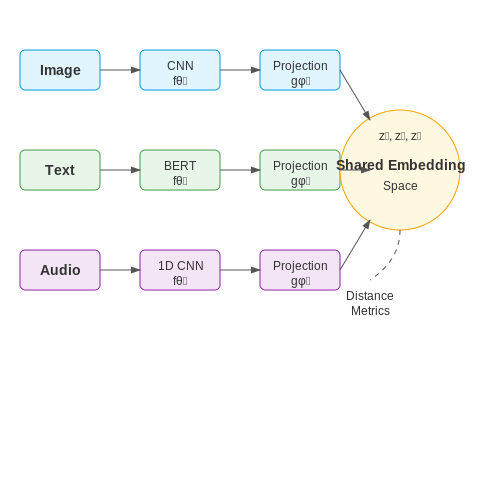
Cross-modal retrieval relies on transforming raw data from different modalities (e.g., images, text, audio) into a shared embedding space where semantically similar items are close, regardless of their original form. The quality of retrieval depends critically on how well features are extracted and represented.
Unimodal Feature Extraction
Each modality requires specialized feature extraction techniques to capture its intrinsic structure:
- Images: Convolutional Neural Networks (CNNs) extract hierarchical spatial features. ResNet or Vision Transformer (ViT) architectures produce high-level semantic representations.
- Text: Word embeddings (Word2Vec, GloVe) or contextualized embeddings (BERT, GPT) encode linguistic meaning.
- Audio: Spectrograms or Mel-Frequency Cepstral Coefficients (MFCCs) are processed by 1D CNNs or recurrent networks.
where \( \mathbf{x}_i \) is the raw input, \( f_\theta \) is the feature extractor (e.g., CNN, Transformer), and \( \mathbf{v}_i \) is the extracted feature vector.
Shared Representation Learning
To enable cross-modal comparison, unimodal features are projected into a common space using transformation functions:
where \( g_\phi \) is a modality-specific projection (often a neural network), and \( \mathbf{z}_i \) is the shared embedding. The goal is to minimize the distance \( d(\mathbf{z}_i, \mathbf{z}_j) \) for semantically related pairs \( (i,j) \) across modalities.
Objective Functions
Common loss functions for learning cross-modal embeddings include:
- Triplet Loss: Minimizes the distance between an anchor and a positive sample while maximizing the distance to a negative sample.
where \( \alpha \) is a margin hyperparameter.
- Contrastive Loss: Directly minimizes distances for positive pairs and pushes apart negative pairs.
where \( y_{ij} \) indicates whether \( (i,j) \) is a positive pair.
Advanced Techniques
Recent advances improve cross-modal alignment through:
- Attention Mechanisms: Dynamically weight relevant features (e.g., cross-modal transformers).
- Adversarial Learning: Use discriminators to ensure modality-invariant embeddings.
- Graph-Based Methods: Exploit relational structure between multimodal data points.
For instance, adversarial learning introduces a discriminator \( D \) that tries to distinguish between modalities, while the feature extractor \( f_\theta \) tries to fool it:
2.2 Similarity Measurement Techniques
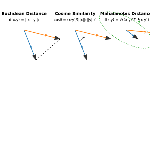
Cross-modal retrieval relies on quantifying the similarity between heterogeneous data representations, such as images and text. Advanced similarity metrics must account for the semantic alignment between modalities while handling their inherent structural differences. Below, we examine the most widely used techniques in research and industry.
Euclidean Distance
The Euclidean distance measures the straight-line distance between two vectors in a multidimensional space. Given two feature vectors x and y in ℝd, the Euclidean distance is computed as:
While simple and interpretable, Euclidean distance assumes isotropy in the feature space, which may not hold for cross-modal embeddings where modalities exhibit different statistical properties.
Cosine Similarity
Cosine similarity measures the angle between two vectors, making it invariant to magnitude differences—a crucial property when comparing normalized embeddings from different modalities:
This metric is particularly effective for text retrieval (e.g., TF-IDF vectors) and image-text matching, where the focus is on directional alignment rather than absolute distances.
Mahalanobis Distance
For modalities with non-uniform feature distributions, the Mahalanobis distance incorporates covariance structure to normalize distances:
Here, Σ is the covariance matrix estimated from training data. This metric is computationally intensive but essential for datasets with correlated or scale-variant features.
Optimal Transport-Based Metrics
Optimal transport (OT) measures similarity by computing the minimal cost to transform one distribution into another. The Wasserstein distance, a popular OT metric, is defined as:
where Γ(μ, ν) denotes all joint distributions with marginals μ and ν. OT-based metrics excel in cross-modal retrieval for their ability to handle unaligned feature spaces and partial correspondences.
Deep Metric Learning
Modern approaches leverage neural networks to learn task-specific similarity functions. Contrastive loss and triplet loss are two widely used objectives:
- Contrastive Loss: Minimizes distance between positive pairs while pushing negative pairs beyond a margin m:
$$ \mathcal{L}_{\text{contrastive}} = (1 - y) \cdot d(x_i, x_j)^2 + y \cdot \max(0, m - d(x_i, x_j))^2 $$
- Triplet Loss: Ensures an anchor is closer to a positive sample than to a negative sample by a margin:
$$ \mathcal{L}_{\text{triplet}} = \max(0, d(x_a, x_p) - d(x_a, x_n) + m) $$
These methods are backbone techniques in models like CLIP and SBERT, enabling robust cross-modal alignment.
Cross-Domain Similarity Localization
For fine-grained retrieval (e.g., region-text matching), attention mechanisms localize relevant subspaces. The similarity score between an image region r and text token t is computed as:
where Wr and Wt are learned projection matrices. This technique underpins models like ViLBERT and UNITER.
2.3 Deep Learning Models for Cross-Modal Retrieval
Neural Network Architectures for Cross-Modal Alignment
Deep learning models excel at learning joint representations across modalities by projecting heterogeneous data into a shared embedding space. The core challenge lies in minimizing the distance between semantically similar cross-modal pairs while maximizing separation for dissimilar ones. Let X and Y represent feature spaces for two modalities (e.g., images and text). The objective function for alignment can be formulated as:
where f and g are deep neural networks mapping each modality to a common space, α is a margin parameter, and (·)+ denotes the hinge function. This triplet loss formulation drives the network to learn discriminative embeddings.
Canonical Architectures
Three dominant architectures have emerged for cross-modal retrieval:
- Two-Stream Networks: Separate encoders process each modality, with late fusion through joint loss functions. ResNet-50 for images and BERT for text are common backbones.
- Cross-Attention Models: Employ transformer architectures with modality-specific attention heads, enabling dynamic feature interaction. The cross-attention score between image region i and text token j is computed as:
- Graph-Based Approaches: Construct modality graphs where nodes represent features and edges encode similarity, then apply graph convolutional networks for joint embedding.
Advanced Training Paradigms
Recent breakthroughs leverage:
- Contrastive Learning: CLIP-style models use noise-contrastive estimation with batch-wise negative sampling. The InfoNCE loss for a batch of N pairs is:
where si and ti are normalized embeddings, and τ is a temperature parameter.
- Adversarial Training: Introduce modality discriminators that try to distinguish the source modality of embeddings, while the main network learns to fool them, enhancing modality invariance.
Evaluation Metrics
Performance is quantified through:
- Recall@K: Percentage of queries where the correct result appears in the top-K retrieved items
- Mean Average Precision (mAP): Area under the precision-recall curve averaged across queries
- Median Rank: Median position of the first correct result in the ranked list
State-of-the-art models on MS-COCO achieve R@1 > 80% for image-to-text retrieval using ViT-L/14 vision encoders paired with 12-layer transformers, demonstrating the power of scaled architectures.

3. Common Evaluation Metrics
3.1 Common Evaluation Metrics
Evaluating cross-modal retrieval systems requires robust metrics that quantify alignment accuracy between heterogeneous data modalities (e.g., text-to-image or audio-to-video). Advanced practitioners rely on the following key metrics:
Recall@K (R@K)
Recall@K measures the probability that at least one relevant item appears in the top-K retrieved results. For a query q and a set of ground-truth relevant items R, it is defined as:
where Q is the query set, and 𝕀 is an indicator function. Higher R@K values indicate better retrieval performance, with K typically set to 1, 5, or 10 in benchmarks like MS-COCO or Flickr30k.
Mean Reciprocal Rank (MRR)
MRR evaluates the average reciprocal rank of the first relevant item across queries. For a single query q, the reciprocal rank is 1/rankq, where rankq is the position of the first correct retrieval. The metric aggregates this over all queries:
MRR is sensitive to the rank of the first relevant result, making it suitable for applications where early precision is critical (e.g., real-time search systems).
Normalized Discounted Cumulative Gain (nDCG)
nDCG accounts for graded relevance (e.g., partially relevant items) and penalizes late-ranked relevant results. The discounted cumulative gain (DCG) is computed as:
where reli is the relevance score of the item at rank i. nDCG normalizes DCG by the ideal DCG (IDCG), which is the maximum possible DCG for the query:
nDCG ranges from 0 to 1, with 1 indicating perfect ranking. It is widely used in benchmarks with multi-level relevance annotations.
Median Rank (MedR)
MedR reports the median rank of the first correct retrieval across all queries. Unlike R@K, it is less sensitive to outliers and provides a robust measure of central tendency. Lower MedR values indicate better performance, with optimal systems achieving MedR = 1.
Mean Average Precision (mAP)
mAP extends precision-recall analysis to ranked lists. For a single query, average precision (AP) is the area under the precision-recall curve, computed as:
where P(k) is precision at cutoff k, and ΔR(k) is the change in recall. mAP averages AP over all queries, making it suitable for datasets with multiple relevant items per query (e.g., image tagging).
Modality Alignment Metrics
Cross-modal retrieval also employs modality-specific metrics:
- CLIPScore: Measures semantic alignment between text and image embeddings using cosine similarity in a joint embedding space.
- BLEU-4: For text-to-text retrieval, adapted from machine translation to assess n-gram overlap.
- Inception Score (IS): Evaluates image quality and diversity in generative cross-modal tasks.
These metrics are often combined in benchmarks like CrossModal-360 or WIT to provide a holistic assessment of retrieval quality across modalities.
3.2 Popular Datasets for Cross-Modal Retrieval
Cross-modal retrieval relies on high-quality datasets that contain aligned data across multiple modalities (e.g., text, images, audio). Below are some of the most widely used datasets in research and industry, along with their key characteristics and applications.
MS-COCO (Microsoft Common Objects in Context)
MS-COCO is a large-scale dataset containing over 330,000 images, each annotated with five descriptive captions. It supports tasks like image-to-text and text-to-image retrieval. The dataset includes object segmentation masks, enabling fine-grained alignment between visual and textual data. A common evaluation metric for retrieval tasks on MS-COCO is Recall@K (K=1, 5, 10), measuring the percentage of queries where the correct item appears in the top-K retrieved results.
Flickr30k
Flickr30k consists of 31,000 images, each paired with five human-annotated captions. It is often used as a benchmark for cross-modal retrieval due to its manageable size and high-quality annotations. Unlike MS-COCO, Flickr30k lacks segmentation masks, making it more suitable for coarse-grained retrieval tasks. Researchers frequently use it to evaluate models before scaling to larger datasets.
Conceptual Captions
Conceptual Captions contains over 3 million image-text pairs automatically harvested from the web. The dataset is notable for its diversity and scale, though the annotations are noisier than manually curated datasets. It is particularly useful for training large-scale models like CLIP or ALIGN, where data quantity is critical for generalization.
AudioSet
AudioSet is a multi-modal dataset containing over 2 million 10-second YouTube clips labeled with 527 audio event classes. It supports audio-visual retrieval tasks, such as retrieving relevant videos given an audio query. The dataset is widely used in sound recognition and cross-modal alignment research.
HowTo100M
HowTo100M provides 136 million video clips with associated narrations from instructional YouTube videos. It is one of the largest datasets for video-text retrieval and is commonly used to train models for tasks like video captioning and temporal grounding. The narrations are automatically transcribed, introducing some noise, but the sheer volume compensates for this limitation.
Wikipedia Image-Text
This dataset pairs images from Wikipedia articles with their corresponding text descriptions. It is particularly useful for domain-specific retrieval tasks, such as scientific or historical image-text matching. The dataset is smaller than web-scale alternatives but offers higher annotation quality due to its curated nature.
SBU Captions
SBU Captions contains 1 million images with weakly associated captions mined from Flickr. The captions are noisy but useful for training robust models that can handle real-world data imperfections. It is often used in studies focusing on noise-resistant retrieval algorithms.
3.3 Performance Comparison Across Models
Cross-modal retrieval models are evaluated using standardized metrics such as Recall@K, Mean Average Precision (mAP), and Normalized Discounted Cumulative Gain (nDCG). The choice of evaluation metric depends on the application: Recall@K emphasizes top-K retrieval accuracy, while mAP assesses ranking quality across all relevant items. For multimodal alignment tasks, nDCG is preferred when graded relevance is available.
Benchmark Datasets and Protocols
Standardized datasets like MS-COCO, Flickr30k, and Conceptual Captions enable fair comparisons. The evaluation protocol typically involves:
- Splitting the dataset into training, validation, and test sets
- Using identical preprocessing and feature extraction pipelines
- Reporting results under both zero-shot and fine-tuned settings
Quantitative Comparison of Model Architectures
Transformer-based models (e.g., CLIP, ALIGN) consistently outperform CNN-RNN hybrids on retrieval tasks. For instance, on MS-COCO's 1K test set:
The performance gap widens in cross-domain retrieval, where transformer models show better generalization. This is quantified by the domain adaptation ratio:
Efficiency-Accuracy Tradeoffs
Model size versus retrieval latency follows a power-law relationship. For a given architecture family (e.g., ViT), inference time T scales with parameter count N as:
Efficient variants like DistilCLIP achieve 80% of the base model's performance with 40% fewer parameters, making them preferable for real-time applications.
Modality-Specific Performance Characteristics
Image-to-text retrieval generally shows higher absolute metrics than text-to-image retrieval across all models. This asymmetry stems from:
- Higher inherent dimensionality of visual data
- Greater variability in possible textual descriptions
- Information loss during visual feature extraction
The modality gap is quantified by the retrieval symmetry index (RSI):
State-of-the-art models achieve RSI > 0.85 on balanced datasets, indicating nearly symmetric performance.
Impact of Pretraining Data Scale
Performance follows a logarithmic relationship with pretraining dataset size D:
Where β ranges from 2.1 to 3.4 depending on model architecture. The law of diminishing returns becomes evident beyond ~100M image-text pairs.
4. Zero-Shot Cross-Modal Retrieval
4.1 Zero-Shot Cross-Modal Retrieval
Zero-shot cross-modal retrieval (ZS-CMR) extends traditional cross-modal retrieval by enabling queries across modalities without requiring task-specific training data. Instead, it leverages pre-trained models and semantic embeddings to generalize to unseen categories by aligning representations in a shared latent space. This capability is particularly valuable in scenarios where labeled data is scarce or unavailable for certain modalities.
Key Challenges and Solutions
The primary challenge in ZS-CMR is bridging the semantic gap between modalities for unseen classes. Traditional approaches rely on supervised learning with paired data, but zero-shot methods must infer relationships using auxiliary information, such as attribute annotations or textual descriptions. Two dominant strategies have emerged:
- Semantic Embedding Alignment: Projects features from different modalities into a shared space using pre-trained models (e.g., CLIP, ViLBERT). For example, given an image I and text T, their embeddings are aligned via cosine similarity:
where f and g are modality-specific encoders.
- Knowledge Graph Propagation: Leverages structured knowledge bases (e.g., WordNet) to propagate semantic relationships between seen and unseen classes. This is formalized as a graph embedding problem:
where E denotes node embeddings and G is the knowledge graph.
Architectural Innovations
Recent advances in ZS-CMR focus on contrastive learning and adversarial training. Contrastive frameworks like CLIP optimize a noise-contrastive estimation (NCE) loss:
where τ is a temperature parameter. Adversarial methods, such as CM-GANs, employ a discriminator to ensure modality-invariant representations by minimizing:
Evaluation Metrics and Benchmarks
ZS-CMR performance is quantified using:
- Recall@K: Proportion of queries where the true match is in the top-K results.
- Mean Average Precision (mAP): Measures ranking quality across all relevant items.
Standard benchmarks include MS-COCO (images ↔ captions) and AudioSet (audio ↔ tags). State-of-the-art models achieve ~60% R@1 on MS-COCO under zero-shot conditions, compared to ~80% in supervised settings.
Practical Applications
ZS-CMR enables applications like:
- Multimedia Search: Retrieving unlabeled images using natural language queries.
- Accessibility Tools: Generating alt-text for images without prior training on specific objects.
- Autonomous Systems: Cross-modal localization (e.g., LiDAR ↔ maps) in novel environments.
For instance, OpenAI's CLIP demonstrates zero-shot transfer to tasks like fine-grained classification by reformulating labels as text prompts (e.g., "a photo of a {class}").

4.2 Multimodal Fusion Techniques
Early Fusion vs. Late Fusion
Multimodal fusion techniques are broadly categorized into early fusion and late fusion, depending on the stage at which modalities are combined. Early fusion integrates raw or low-level features before feeding them into a model, while late fusion processes each modality separately and combines their outputs at a higher abstraction level.
Early fusion is advantageous when modalities exhibit strong local correlations, such as synchronized audio-visual data. However, it suffers from sensitivity to noise and misalignment. Late fusion, on the other hand, is robust to modality-specific noise but may fail to capture fine-grained cross-modal interactions.
Hybrid Fusion Strategies
Hybrid approaches combine early and late fusion to leverage their complementary strengths. For instance, intermediate fusion integrates modalities at multiple hierarchical levels, enabling both low-level and high-level feature interactions. A common implementation uses attention mechanisms to dynamically weight modality contributions:
Transformer-based architectures, such as ViLBERT and CLIP, employ cross-modal attention layers to model bidirectional interactions between modalities. These models pre-train on large-scale multimodal datasets to learn shared representations that generalize across tasks.
Tensor-Based Fusion
For modalities with complex interactions, tensor-based methods capture higher-order correlations. The tucker decomposition factorizes a multimodal tensor 𝒳 into a core tensor and factor matrices:
Here, 𝒢 is the core tensor, and A, B, C are factor matrices for each modality. This decomposition reduces dimensionality while preserving multiway relationships, making it suitable for applications like medical imaging and robotics.
Graph-Based Fusion
Graph neural networks (GNNs) model modalities as nodes in a graph, with edges representing their relationships. The fusion process aggregates information via message passing:
This approach excels in scenarios with heterogeneous data (e.g., social media posts combining text, images, and user networks). Dynamic graph construction further adapts to varying modality importance.
Real-World Applications
- Autonomous Vehicles: Fusing LiDAR, camera, and radar data for robust object detection.
- Healthcare: Integrating MRI scans, genomic data, and clinical notes for personalized diagnosis.
- Content Retrieval: Cross-modal search engines combining text queries with image/video results.

4.3 Self-Supervised Learning in Cross-Modal Retrieval
Self-supervised learning (SSL) has emerged as a powerful paradigm for cross-modal retrieval by leveraging inherent data structure to generate supervisory signals without explicit human annotation. Unlike supervised methods that rely on labeled correspondences between modalities, SSL exploits the natural co-occurrence or alignment of multimodal data (e.g., image-text pairs) to learn joint representations.
Contrastive Learning for Cross-Modal Alignment
The dominant SSL approach in cross-modal retrieval is contrastive learning, which maximizes agreement between positive pairs (e.g., an image and its caption) while minimizing agreement for negative pairs. Given a batch of N image-text pairs, the InfoNCE loss for image-to-text retrieval is formulated as:
where fi and gi are L2-normalized embeddings for the i-th image and text, respectively, and τ is a temperature hyperparameter. The symmetric text-to-image loss Lt2i is computed analogously, with the total loss being L = Li2t + Lt2i.
Momentum Encoders and Memory Banks
To scale contrastive learning to large datasets, momentum encoders maintain slowly-updated versions of the main encoders:
where m ∈ [0,1) is a momentum coefficient. This provides stable targets for learning while avoiding collapse. Memory banks further improve efficiency by caching embeddings from previous batches, enabling larger effective negative sample sizes without increased compute.
Cross-Modal Masked Modeling
Inspired by BERT, masked multimodal modeling reconstructs masked portions of one modality using information from other modalities. For video-text retrieval, a joint transformer might predict masked text tokens from visual features:
where E is a token embedding matrix and w\t denotes all text tokens except the t-th one. This forces the model to learn fine-grained cross-modal relationships.
Practical Considerations
- Batch composition: Larger batch sizes improve contrastive learning but require careful memory management via gradient checkpointing or mixed precision.
- Hard negative mining: Identifying informative negatives (e.g., semantically similar but mismatched pairs) significantly boosts performance over random sampling.
- Modality gap: The inherent discrepancy between modality distributions can be mitigated through techniques like cross-modal mixup or shared latent space constraints.
Recent advances like CLIP and ALIGN demonstrate that SSL-trained models can outperform supervised approaches on zero-shot cross-modal retrieval by orders of magnitude in training data efficiency. The key lies in designing pretext tasks that force the model to discover meaningful semantic correspondences rather than exploiting dataset-specific biases.

5. Key Research Papers
5.1 Key Research Papers
- End-to-end cross-modality retrieval with CCA projections and pairwise ... — Cross-modality retrieval encompasses retrieval tasks where the fetched items are of a different type than the search query, e.g., retrieving pictures relevant to a given text query. The state-of-the-art approach to cross-modality retrieval relies on learning a joint embedding space of the two modalities, where items from either modality are retrieved using nearest-neighbor search. In this work ...
- Representation separation adversarial networks for cross-modal retrieval — Cross-modal retrieval aims to search the semantically similar instances from the other modalities by giving a query from one modality. Recently, generative adversarial networks (GANs) has been proposed to model the joint distribution over the data from different modalities and to learn the common representations for cross-modal retrieval. However, most of existing GANs-based methods simply ...
- Cross-modal image retrieval with deep mutual information maximization — In this paper, we have proposed a new method for cross-modal image retrieval based on the contrastive self-supervised learning approach Deep InfoMax [23], [1]. Our model improves the retrieval performance by aligning the feature distributions of the text modality, the image modality and the fusion modality.
- Hybrid DAER Based Cross-Modal Retrieval Exploiting Deep ... - MDPI — This study contributes to cross-modal information retrieval research by developing a novel image-text retrieval method. This method addresses the dual attention network and the enhanced relational network with different activation functions to fit in the dimension gap between the cross-modal information.
- PDF HCMSL: Hybrid Cross-Modal Similarity Learning for Cross-Modal Retrieval — In this paper, we present a novel cross-modal retrieval method, named Hybrid Cross-Modal Similarity Learning model (HCMSL forshort).Itaimstocapturesu ...
- A Cross‐Modal Image and Text Retrieval Method Based on Efficient ... — In order to make better association learning between different modal data, a cross-modal image and text retrieval method combining efficient feature extraction and interactive learning convolutional autoencoder (CAE) is proposed in this paper.
- Cross-Modal Retrieval-enhanced code Summarization based on joint ... — Objective: To address this issue, this paper introduces CMR-Sum: a novel Cross-Modal Retrieval-enhanced code Summarization framework based on joint learning for generation and retrieval tasks, where both two tasks are allowed to be optimized simultaneously.
- LCM: A Surprisingly Effective Framework for Supervised Cross-modal ... — The recent deep cross-modal hashing (DCMH) has achieved superior performance in effective and efficient cross-modal retrieval and thus has drawn increasing attention.
- PDF Regularized Diffusion Process on Bidirectional Context for Object Retrieval — , we also apply ARDP to cross-modal retrieval on the Wikipedia dataset [26], [27], where retrieval is done between text data and image data. And in Sec. 5.6, the validity of HRDP is testified w th view-based 3D model retrieval on the Princeton Shape Benchmark (PSB) [28]
- An Efficient Cross-Modal Privacy-Preserving Image-Text Retrieval Scheme — Preserving the privacy of the ever-increasing multimedia data on the cloud while providing accurate and fast retrieval services has become a hot topic in information security. However, existing relevant schemes still have significant room for improvement in accuracy and speed. Therefore, this paper proposes a privacy-preserving image-text retrieval scheme called PITR. To enhance model ...
5.2 Recommended Books and Surveys
- PDF Chapter 5 Cross Modal Multimedia Retrieval — 5.2 Previous Work The problems of image and text retrieval have been the subject of ex-tensive research in the elds of information retrieval, computer vision, and mul-timedia [28, 133, 132, 106, 93]. In all these areas, the emphasis has been on uni-modal approaches, where query and retrieved documents share a single modal-ity [125, 124, 156, 28, 133]. For example, in [124], a query text and in ...
- (跨模态检索综述)A Comprehensive Survey on Cross-modal Retrieval — 基于对抗的跨媒体 检索Cross-modal retrieval aims to enable flexible retrieval experience a cross different modal ities (e.g., texts vs. images). The core of crossmodal retrieval research is to learn a comm on subspace where the items of different modal ities can be directly compared to each other. In this paper, we present a novel Adversarial Cross- Modal Retrieval (ACMR) method ...
- End-to-end cross-modality retrieval with CCA projections and pairwise ... — Cross-modality retrieval encompasses retrieval tasks where the fetched items are of a different type than the search query, e.g., retrieving pictures relevant to a given text query. The state-of-the-art approach to cross-modality retrieval relies on learning a joint embedding space of the two modalities, where items from either modality are retrieved using nearest-neighbor search. In this work ...
- HCMSL: Hybrid Cross-modal Similarity Learning for Cross-modal Retrieval — The purpose of cross-modal retrieval is to find the relationship between different modal samples, and to retrieve other modal samples with similar semantics by using a certain modal sample.
- Cross-Modal Retrieval-enhanced code Summarization based on joint ... — This is because the single-modal retrieval mechanism has a much higher retrieval accuracy than the cross-modal retrieval mechanism, which indicates that for the testing stage, we should search for the most relevant prototype summaries to enhance the performance of code summarization.
- PDF Revisiting Cross Modal Retrieval - arXiv.org — This paper proposes a cross modal retrieval system that leverages on image and text encoding. Most multimodal architectures employ separate networks for each modality to capture the semantic relationship between them.
- (PDF) Revisiting Cross Modal Retrieval - ResearchGate — This paper proposes a cross-modal retrieval system that leverages on image and text encoding. Most multimodal architectures employ separate networks for each modality to capture the semantic ...
- (PDF) Feature-Centric Framework for Multi-Modal Retrieval System — Multi-modal information retrieval has great implications for search engines, situational knowledge delivery and complex data management systems. Existing cross-modal learning models use separate information models for each data modality and lack the compatibility to utilize pre-existing features in an application domain.
- A survey of transformer-based multimodal pre-trained modals — Image-text understanding tasks, such as Visual Question Answering (VQA) [81], image-text retrieval [142], referring expression comprehension [143], require the PTM to learn the representation of language semantics, vision contents, and cross-modal alignments without requiring generation ability.
- Maybe You Are Looking for CroQS Cross-Modal Query Suggestion for Text ... — In this work, we address query suggestion in cross-modal retrieval, introducing a novel task that focuses on suggesting minimal textual modifications needed to explore visually consistent subsets of the collection, following the premise of "Maybe you are looking for".
5.3 Online Resources and Tutorials
- BMC-SDNU/Cross-Modal-Retrieval: Cross-Modal-Real-valuded-Retrieval - GitHub — DREN:Dual-Level Representation Enhancement on Characteristic and Context for Image-Text Retrieval(TCSVT) M2D-BERT:Multi-scale Multi-modal Dictionary BERT For Effective Text-image Retrieval in Multimedia Advertising(CIKM) ViSTA:ViSTA: Vision and Scene Text Aggregation for Cross-Modal Retrieval(CVPR) COTS: Collaborative Two-Stream Vision-Language Pre-Training Model for Cross-Modal Retrieval(CVPR)
- Cross-Modal Representation Learning - SpringerLink — 7.4.2 Cross-Modal Retrieval. With the rapid growth of multimodal data such as text, image, video, and audio on the Internet, the need to retrieve information across different modalities (i.e., cross-modal retrieval) has become stronger. Given the query data from one modality, cross-modal retrieval aims to retrieve relevant data in other modalities.
- PDF Chapter 5 Cross Modal Multimedia Retrieval - University of California ... — image [4, 97, 21] and song [151, 149, 89, 36] retrieval systems. One property of cross-modal retrieval is that, by de nition, it requires representations that gener-alize across content modalities. This implies the ability to establish cross-modal links between the attributes (of di erent modalities) characteristic of each doc-ument, or ...
- A Cross‐Modal Image and Text Retrieval Method ... - Wiley Online Library — Therefore, effective feature extraction and feature association learning are key to improving the accuracy of cross-modal retrieval. In order to make better association learning between different modal data, a cross-modal image and text retrieval method combining efficient feature extraction and interactive learning convolutional autoencoder (CAE) is proposed in this paper.
- PDF Continual Learning in Cross-Modal Retrieval - CVF Open Access — ting from the perspective of cross-modal embeddings. 3. Continual cross-modal retrieval 3.1. Crossmodal deep metric learning Our framework is based on a two-branch network [63], with image-specific and text-specific embedding branches that project images and text into a common space. The im-age embedding operation is u = fθ (x), where u ∈ RE
- (PDF) Cross-View Image Retrieval - Ground to Aerial Image Retrieval ... — Existing technique applies cross-modal retrieval techniques to multi-modal data but do not address variety of data in any single modality such as multi-view image retrieval [15]. Cross-view image matching could be taken as one of the potential problems for which Vo. et. al cross-matched and geo-localized street-view images of the 11 cities of ...
- PDF Effective Deep Learning Based Multi-Modal Retrieval — web document retrieval via keyword queries and content-based image retrieval. 2. Cross-modal search enables users to explore relevant resources from different modalities. For example, a user can use a tweet to retrieve relevant photos and videos from other heterogeneous data sources. Meanwhile he can search relevant textual descriptions or ...
- A Framework for Enabling Unpaired Multi-Modal Learning for Deep Cross ... — Cross-Modal Retrieval (CMR) is a sub-field of MMIR which focuses on retrieving information from one modality using a query from another modality. An example of CMR is retrieving images when using text as a query and vice versa. ... The need for longer hash codes results in additional computational resources being required, which results in a ...
- TeachText: CrossModal text-video retrieval through generalized ... — Download: Download high-res image (69KB) Download: Download full-size image Fig. 1. Distilling the knowledge from multiple text encoders for stronger text-video retrieval. Prior work [5], [6], [7] has shown the considerable benefit of transitioning from video encoders that ingest a single modality (left) to multi-modal video encoders (centre).In this work, we show that retrieval performance ...
- Improving semantic video retrieval models by training with a relevance ... — To retrieve a video via a multimedia search engine, a textual query is usually created by the user and then used to perform the search. Recent state-of-the-art cross-modal retrieval methods learn a joint text-video embedding space by using contrastive loss functions, which maximize the similarity of positive pairs while decreasing that of the negative pairs.