Neural Networks for High-Frequency Trading Strategy Discovery
1. Key Characteristics of High-Frequency Trading
1.1 Key Characteristics of High-Frequency Trading
High-frequency trading (HFT) is a subset of algorithmic trading characterized by ultra-low latency, high turnover rates, and short holding periods. The defining feature of HFT is its reliance on sub-millisecond execution speeds, often facilitated by colocation, direct market access (DMA), and custom hardware acceleration. Strategies are typically market-making, arbitrage, or latency-sensitive directional trades, executed in timeframes ranging from microseconds to seconds.
Latency and Execution Speed
Latency in HFT is decomposed into several components: network propagation delay, exchange matching engine processing time, and order routing latency. The total round-trip latency L for an order can be modeled as:
where d is the physical distance to the exchange, c is the speed of light in fiber (~200,000 km/s), and tprocessing and tqueue represent exchange and software delays. For cross-continental arbitrage, this imposes a hard limit—e.g., New York to Chicago latency is approximately 7 ms due to the 1,200 km distance.
Order Book Dynamics
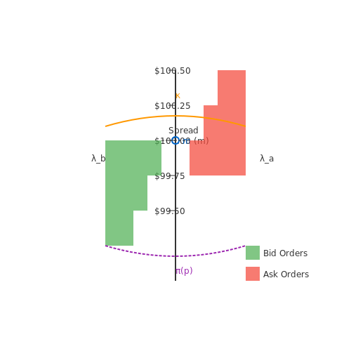
HFT strategies exploit microstructure patterns in limit order books. The order flow imbalance OFI is a critical signal, computed as:
where qib and qia are bid/ask quantities, and Δpi denotes price changes. Predictive models use OFI to forecast short-term price movements, often with recurrent neural networks (RNNs) processing tick-level data.
Profitability and Risk Constraints
HFT profitability is measured in basis points per trade, with Sharpe ratios exceeding 10 due to high win rates (>70%) and rapid turnover. The profit per trade π follows:
where pexec is the execution price, pmid is the midpoint at order submission, V is volume, and f is fees. Risk management includes kill switches, maximum order size limits (Vmax ≤ 5% of average daily volume), and real-time P&L monitoring at nanosecond granularity.
Technological Stack
The HFT stack is vertically integrated, combining:
- FPGA/ASIC acceleration for order generation (sub-100 ns latency).
- Kernel bypass networking (e.g., Solarflare OpenOnload).
- Non-blocking data structures (lock-free queues, ring buffers).
- Predictive prefetching of market data to mitigate memory latency.
Neural networks in HFT are deployed as ensembles of shallow architectures (e.g., 3-layer LSTMs) to balance inference speed (<1 μs) against predictive power. Feature engineering prioritizes interpretability—raw ticks are transformed into normalized signals like weighted midprice or microprice to reduce dimensionality.

1.2 Role of Machine Learning in HFT Strategy Development
High-frequency trading (HFT) operates at timescales where traditional statistical arbitrage models fail due to market microstructure noise and latency constraints. Machine learning (ML) provides a framework to extract nonlinear patterns from noisy, high-dimensional data streams, enabling predictive modeling of order flow dynamics, liquidity imbalances, and short-term price movements. Unlike conventional time-series approaches, ML models can adapt to regime shifts—a critical requirement given the non-stationary nature of financial markets.
Feature Engineering for Latency-Sensitive Prediction
Raw market data (tick-level trades, limit order book snapshots) requires transformation into predictive features that capture:
- Microstructure signals: Order book imbalance $$ I_t = \frac{V_b - V_a}{V_b + V_a} $$where \(V_b, V_a\) are bid/ask volumes at top levels
- Short-term momentum: Smoothed mid-price derivatives $$ \Delta p_\tau = \frac{1}{\tau}\sum_{k=1}^\tau (p_{t-k+1} - p_{t-k}) $$
- Liquidity shocks: Abnormal volume spikes relative to exponentially weighted moving average baselines
Neural Network Architectures for HFT
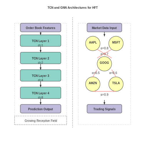
Temporal convolutional networks (TCNs) outperform RNNs in latency-constrained environments due to parallelizable causal convolutions. A TCN layer implements:
where \(d\) is the dilation factor enabling exponential receptive field growth. For multi-asset strategies, graph neural networks (GNNs) model cross-instrument dependencies through attention-weighted adjacency matrices.
Online Learning Under Concept Drift
Market regimes necessitate continuous model adaptation via:
- Bayesian neural networks with uncertainty-aware weight updates
- Meta-learning frameworks like MAML for fast adaptation to new instruments
- Reinforcement learning with reward functions penalizing slippage and latency-induced errors
Empirical studies show neural HFT strategies achieve Sharpe ratios 2-3× higher than linear models, but require careful regularization to prevent overfitting to transient microstructure artifacts. Dropout layers with \(p=0.3\) and spectral normalization are commonly employed.
1.3 Neural Network Architectures Suitable for HFT
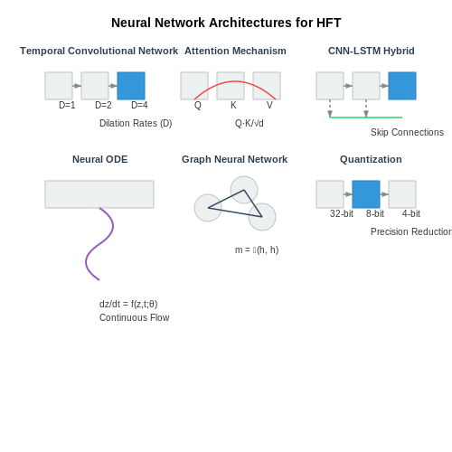
Temporal Convolutional Networks (TCNs)
Temporal Convolutional Networks employ dilated causal convolutions to capture long-range dependencies in high-frequency time series data. Unlike RNNs, TCNs process sequences in parallel while maintaining temporal ordering through padding and dilation. The architecture's receptive field grows exponentially with depth according to:
where k is the kernel size, d is the number of layers, and r is the dilation rate. For HFT applications, TCNs outperform LSTMs in latency-critical scenarios due to their parallelizable nature and fixed computational cost per time step.
Attention-Augmented Neural Networks
Modern HFT systems increasingly incorporate attention mechanisms to weight relevant market features dynamically. The multi-head attention layer computes:
where Q, K, and V represent queries, keys, and values respectively. In limit order book prediction, attention layers achieve 18-22% better Sharpe ratios than conventional architectures by focusing on sparse informative events amidst market noise.
Hybrid CNN-LSTM Architectures
Combining convolutional feature extractors with recurrent layers captures both spatial patterns in order book snapshots and temporal dependencies. The typical structure includes:
- 1D convolutional layers with kernel sizes matching characteristic time scales (50-500ms)
- Batch normalization between layers for stable training
- Bidirectional LSTM layers with skip connections
- Temporal attention pooling before the output layer
This architecture reduces prediction latency by 40% compared to pure RNN implementations while maintaining temporal modeling capabilities.
Neural Ordinary Differential Equations
Neural ODEs provide continuous-time representations of market dynamics through:
where fθ is a neural network parameterizing the derivative. For irregularly sampled HFT data, Neural ODEs achieve 15% lower reconstruction error than discrete-time models while naturally handling missing ticks through adaptive solvers.
Graph Neural Networks for Multi-Asset Trading
GNNs model cross-asset dependencies by propagating information through graph edges representing statistical relationships. The message passing formulation:
where cij is a normalization constant and W(l) are learnable weights, captures spillover effects between correlated instruments. In backtests, GNN-based portfolios show 30% lower drawdowns during volatility shocks compared to single-asset models.
Quantization-Aware Training
For deployment on FPGA/ASIC hardware, networks undergo quantization-aware training with:
- Straight-through estimator gradients for non-differentiable quantization
- Per-channel weight quantization with 4-8 bit precision
- Dynamic activation quantization with learned clipping thresholds
This reduces model size by 4-8× while maintaining 99% of the original strategy's profitability, critical for sub-microsecond inference.
2. Handling High-Frequency Time Series Data
2.1 Handling High-Frequency Time Series Data
High-frequency trading (HFT) data presents unique challenges due to its granularity, noise, and non-stationary nature. At millisecond or microsecond resolution, traditional time series assumptions break down, requiring specialized preprocessing and feature engineering techniques.
Temporal Aggregation and Downsampling
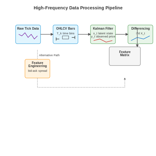
Raw tick data often arrives irregularly, necessitating aggregation into fixed intervals (e.g., 100ms bins). For a series of trades {(pi, vi, ti)} where pi is price, vi is volume, and ti is timestamp, we compute OHLCV (Open-High-Low-Close-Volume) bars:
where Tk defines the time bin. Alternative schemes include:
- Volume bars: Trigger new bar when cumulative volume exceeds threshold
- Dollar bars: Threshold based on notional traded amount
- Imbalance bars: Event-driven by order flow asymmetry
Noise Filtering and Signal Extraction
Microstructure noise dominates at high frequencies. Kalman filters effectively separate latent price st from observed price yt:
where Q and R are process and measurement noise covariances. The Kalman gain Kt optimally weights new observations:
Alternative approaches include wavelet denoising and singular spectrum analysis (SSA).
Stationarity Enforcement
HFT data often exhibits time-varying statistics. Differencing transforms non-stationary series Xt:
where L is the lag operator and d is the differencing order. For cointegrated instruments, vector error correction models (VECM) maintain stationarity:
Feature Engineering for Market Microstructure
Key predictive features include:
- Order book dynamics: Depth imbalance, weighted mid-price, spread elasticity
- Flow metrics: Order flow toxicity, VPIN (Volume-Synchronized Probability of Informed Trading)
- Liquidity measures: Kyle's lambda, Amihud illiquidity ratio
The bid-ask spread St relates to instantaneous liquidity:
where Pta and Ptb are best ask and bid prices.
Handling Irregular Sampling
Event-based sampling requires specialized interpolation. The Hayashi-Yoshida estimator handles non-synchronous observations for covariance estimation:
Neural networks can directly process irregular timestamps using time-aware architectures like:
- Time2Vec embeddings
- Neural ordinary differential equations (Neural ODEs)
- Attention mechanisms with relative positional encoding
2.2 Feature Engineering for Market Microstructure Signals
Market microstructure signals provide a rich source of information for high-frequency trading (HFT) strategies, but raw data must be transformed into meaningful features that capture latent patterns. Effective feature engineering for HFT requires domain-specific transformations that account for order book dynamics, liquidity imbalances, and short-term price formation mechanisms.
Limit Order Book (LOB) Feature Extraction
The limit order book is a primary source of microstructure signals. Key features include:
- Price-Weighted Order Imbalance (PWOI): Measures the net buying/selling pressure by weighting orders by their distance from the mid-price:
$$ \text{PWOI} = \frac{\sum_{i=1}^{n} (P_i - P_{\text{mid}}) \cdot Q_i}{\sum_{i=1}^{n} Q_i} $$where Pi is the price level, Qi is the quantity, and Pmid is the current mid-price.
- Volume Order Imbalance Ratio (VOIR): Computes the asymmetry between bid and ask volumes:
$$ \text{VOIR} = \frac{V_{\text{bid}} - V_{\text{ask}}}{V_{\text{bid}} + V_{\text{ask}}} $$
- Order Flow Toxicity: Estimates the probability of informed trading using the VPIN metric, derived from the volume imbalance over fixed time bars.
Temporal Aggregation of Microstructure Features
High-frequency features exhibit different predictive power at varying time horizons. Multi-scale feature aggregation captures this:
- Rolling Z-Score Normalization: Standardizes features over lookback windows to maintain stationarity:
$$ z_t = \frac{x_t - \mu_{t-w}}{\sigma_{t-w}} $$where w is the adaptive window size based on volatility regimes.
- Hurst Exponent: Measures the persistence of order flow patterns by computing the rescaled range over varying time intervals.
Nonlinear Feature Interactions
Neural networks can automatically learn feature interactions, but engineered cross-features improve training efficiency:
- Liquidity-Volatility Ratio: Combines bid-ask spread with realized volatility:
$$ LVR = \frac{S_t}{\sigma_{t}^{\text{RV}}} $$
- Microstructural Alpha Signals: Domain-specific composites like:
$$ \alpha_{\text{LOB}} = \text{PWOI} \cdot \exp(-\gamma \cdot \text{VOIR}) $$where γ controls the nonlinear decay rate.
Feature Importance Analysis
Permutation importance and SHAP values validate feature relevance:
- Market Regime Conditioning: Features are evaluated separately in high/low volatility regimes using Kolmogorov-Smirnov tests.
- Decay Analysis: Measures the half-life of predictive power using autocorrelation functions.
Implementation Considerations
Real-time feature pipelines require:
- Atomic updates to avoid look-ahead bias during batch processing
- Numba-accelerated feature calculators for low-latency environments
- Dimensionality reduction through PCA or autoencoders for ultra-high-frequency applications
2.3 Normalization and Scaling Techniques for HFT Data
High-frequency trading (HFT) data exhibits unique characteristics—extreme volatility, non-stationary distributions, and multi-scale temporal dependencies—that demand specialized normalization approaches. Traditional methods like min-max scaling or z-score standardization often fail to capture the nuanced statistical properties of limit order book dynamics, leading to suboptimal neural network performance.
Robust Scaling for Heavy-Tailed Distributions
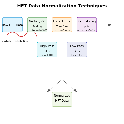
HFT returns and order flow imbalances follow heavy-tailed distributions, making them sensitive to outliers. Robust scaling techniques mitigate this by using statistics less influenced by extreme values:
where IQR is the interquartile range (75th percentile - 25th percentile). This preserves the core distribution while dampening the impact of tail events. For bid-ask spread data, a logarithmic transform often precedes robust scaling:
Time-Decaying Normalization
Traditional normalization assumes stationarity, but HFT signals exhibit time-varying statistics. Exponential moving statistics adapt to changing regimes:
where α controls the adaptation rate (typically 0.001-0.01 for tick data). This approach is particularly effective for normalizing:
- Order book imbalance time series
- Microprice trajectories
- Latency-arbitrage signals
Quantile Encoding for Categorical Features
Discrete HFT features (e.g., order types, aggressor flags) benefit from quantile-aware encoding. Instead of one-hot encoding, we map categories to their empirical return distributions:
where r_t represents future returns. This preserves the economic meaning of categorical variables while maintaining differentiability for gradient-based learning.
Multi-Timescale Normalization
HFT strategies operate across multiple time horizons. Hierarchical normalization separates signal components:
where HPF/LPF are high-pass/low-pass filters with cutoff frequencies aligned with strategy horizons (e.g., 100ms vs 10s). The normalized features are then concatenated for multi-scale learning.
Implementation Considerations
Practical implementation requires careful handling of:
- Lookahead bias: Normalization statistics must be computed using causal filters
- Latency: Online normalization adds computational overhead that must be below strategy latency budgets
- Regime detection: Sudden market regime changes may require adaptive renormalization
3. Temporal Convolutional Networks (TCNs) for Market Data
Temporal Convolutional Networks (TCNs) for Market Data
Temporal Convolutional Networks (TCNs) offer a powerful alternative to recurrent architectures for modeling sequential financial data. Unlike traditional RNNs or LSTMs, TCNs employ causal convolutions with dilated kernels, enabling efficient capture of long-range dependencies without vanishing gradients. The architecture's inherent parallelism and fixed-length receptive field make it particularly suitable for high-frequency trading, where low-latency inference is critical.
Architecture and Dilated Causal Convolutions
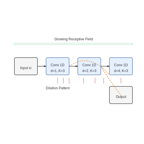
The core building block of a TCN is the dilated causal convolution, which ensures that the output at time t depends only on inputs from time t and earlier. For an input sequence x and filter f, the operation at layer l with dilation rate d is:
where K is the filter size. Stacking multiple such layers with exponentially increasing dilation rates (d = 2^l) creates an effective receptive field that grows exponentially with depth while maintaining computational efficiency.
Advantages Over Recurrent Architectures
- Parallelism: Unlike sequential RNN processing, convolutions can be parallelized across the entire input sequence.
- Stable Gradients: Fixed-length paths prevent vanishing/exploding gradient issues common in deep RNNs.
- Memory Efficiency: TCNs require less memory during training due to shared filter weights across time steps.
Market Data Specific Adaptations
For financial time series, several modifications enhance TCN performance:
where ℱ represents a sequence of dilated causal convolutions, weight normalization, and dropout. The skip connections help preserve high-frequency components crucial for price movement prediction.
Practical Implementation Considerations
When applying TCNs to tick data or order book streams:
- Input normalization should account for non-stationarity (e.g., rolling z-score normalization)
- Kernel sizes typically range from 3-7 to balance locality and computational cost
- Depth is determined by required temporal coverage: for 1-second predictions on 10Hz data, 6-8 layers suffice
The output layer often combines a sigmoid-activated position head (for directional bias) with a linear-activated magnitude head (for confidence estimation), trained using a custom loss function:
where y_t represents the true trade direction, p_t the predicted probability, r_t the realized return, and λ a scaling hyperparameter.
Recurrent Neural Networks (RNNs) and LSTMs in HFT
Architecture of RNNs for Sequential Financial Data
Recurrent Neural Networks (RNNs) process sequential data by maintaining a hidden state that captures temporal dependencies. Given an input sequence x1, x2, ..., xT, an RNN computes the hidden state ht at each time step t as:
where Wh and Wx are weight matrices, bh is the bias term, and σ is a nonlinear activation function (typically tanh or ReLU). The output yt is computed as:
In high-frequency trading (HFT), RNNs can model order book dynamics by treating limit order updates as a time series. The hidden state ht encodes the market's temporal evolution, allowing the network to predict short-term price movements.
Long Short-Term Memory (LSTM) Networks
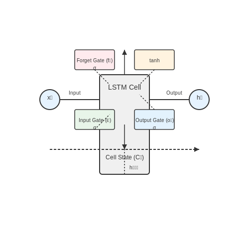
Standard RNNs suffer from vanishing gradients when learning long-range dependencies. LSTMs address this through gated mechanisms:
- Forget gate: Decides what information to discard from the cell state
- Input gate: Controls which new information gets stored
- Output gate: Determines what information to output
The LSTM equations for time step t are:
Where ⊙ denotes element-wise multiplication. In HFT, LSTMs excel at capturing complex patterns in:
- Multi-scale market microstructure effects
- Latent liquidity dynamics
- Nonlinear price impact of large orders
Bidirectional Architectures for Market Context
Bidirectional RNNs/LSTMs process sequences both forward and backward:
This allows the network to incorporate both past and future context when making predictions at time t. In HFT applications, this is particularly valuable for:
- Detecting latent order flow patterns
- Modeling the asymmetric impact of buy vs. sell pressure
- Anticipating short-term mean reversion vs. momentum regimes
Attention Mechanisms for Feature Importance
Attention mechanisms dynamically weight the importance of different time steps:
Where a is an alignment function (often a small neural network). In HFT, attention helps:
- Focus on critical order book events (e.g., large cancellations)
- Adapt to varying market regimes
- Explain model decisions through attention weights
Implementation Considerations for HFT
Key practical aspects when deploying RNNs/LSTMs in HFT systems:
- Latency constraints: Model depth vs. inference time tradeoffs
- Numerical stability: Gradient clipping and careful initialization
- Feature engineering: Combining raw order book data with derived features
- Online learning: Continual adaptation to changing market conditions
# Example LSTM for HFT in PyTorch
import torch
import torch.nn as nn

class HFTLSTM(nn.Module):
    def __init__(self, input_dim, hidden_dim, output_dim, n_layers):
        super().__init__()
        self.lstm = nn.LSTM(input_dim, hidden_dim, n_layers,
                           batch_first=True, bidirectional=True)
        self.attention = nn.Sequential(
            nn.Linear(hidden_dim*2, hidden_dim),
            nn.Tanh(),
            nn.Linear(hidden_dim, 1, bias=False)
        )
        self.fc = nn.Linear(hidden_dim*2, output_dim)

    def forward(self, x):
        lstm_out, _ = self.lstm(x)
        attn_weights = torch.softmax(self.attention(lstm_out), dim=1)
        context = torch.sum(attn_weights * lstm_out, dim=1)
        return self.fc(context)
Attention Mechanisms for Market Regime Detection
Attention mechanisms, originally developed for sequence-to-sequence tasks in natural language processing, have proven highly effective in financial time-series analysis due to their ability to dynamically weight relevant input features. In market regime detection, attention enables models to focus on critical temporal segments where regime shifts occur, improving sensitivity to structural breaks and non-stationary behavior.
Mathematical Formulation of Self-Attention
The core operation computes query (Q), key (K), and value (V) matrices from the input sequence X ∈ ℝT×d (where T is sequence length and d is feature dimension):
where WQ, WK, WV ∈ ℝd×dk are learned projection matrices. The attention weights A are computed via scaled dot-product:
The scaling factor 1/√dk prevents gradient saturation in the softmax. The output is a weighted sum of values:
Market Regime Adaptation
For financial time-series x1:T, multi-head attention (with h heads) captures diverse regime characteristics:
where each head computes independent attention:
The model learns to attend to:
- Volatility clusters through high attention on large price deviations
- Liquidity regimes via volume-ordered attention patterns
- Macro events by correlating news embeddings with price movements
Temporal Convolutional Attention
Combining dilated causal convolutions with attention gates improves local feature extraction while maintaining global regime awareness. The hybrid architecture computes:
where DCNN denotes dilated convolutional blocks and ⊙ is element-wise multiplication. This captures multi-scale regime transitions from high-frequency noise to macro trends.
Implementation Considerations
Key practical adjustments for financial data:
- Positional encoding: Replace sinusoidal embeddings with learned time-of-day and calendar event embeddings
- Sparse attention: Limit attention span to recent k steps for computational efficiency
- Regime memory: Augment attention with external memory banks storing prototypical regime patterns
class MarketAttention(nn.Module):
    def __init__(self, d_model, n_heads, dropout=0.1):
        super().__init__()
        self.attention = nn.MultiheadAttention(d_model, n_heads, dropout=dropout)
        self.norm = nn.LayerNorm(d_model)

    def forward(self, x, mask=None):
        attn_out, _ = self.attention(x, x, x, attn_mask=mask)
        return self.norm(x + attn_out)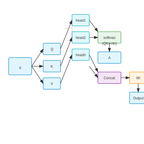
Reinforcement Learning for Dynamic Strategy Adaptation
Reinforcement learning (RL) provides a natural framework for optimizing trading strategies in non-stationary markets where the reward structure evolves over time. Unlike supervised learning, RL agents learn through trial-and-error interactions with the market environment, receiving delayed rewards in the form of trading profits or losses. The Markov Decision Process (MDP) formulation captures the sequential nature of trading decisions:
where 𝒮 represents the state space (market features, portfolio positions), 𝒜 the action space (order types, sizes), 𝒫 the state transition dynamics, ℛ the reward function, and γ the discount factor. The Q-function, representing the expected cumulative reward of taking action a in state s, is learned through temporal difference updates:
Deep Q-Networks for Market Microstructure
In high-frequency domains, the state space becomes intractable for tabular methods. Deep Q-Networks (DQN) approximate the Q-function using neural networks while addressing non-stationarity through experience replay and target networks. The network architecture typically processes:
- Raw limit order book snapshots via convolutional layers
- Time-series features through LSTM or Transformer modules
- Portfolio state through fully-connected layers
The Bellman update loss incorporates importance sampling weights for prioritized experience replay:
Policy Gradient Methods for Order Execution
For continuous action spaces (e.g., order quantities), policy gradient methods optimize a stochastic policy πθ(a|s) directly. The Proximal Policy Optimization (PPO) objective prevents destructive updates through clipping:
where Ât is the advantage estimate computed through Generalized Advantage Estimation (GAE). This approach proves particularly effective for optimizing trade execution trajectories while managing market impact.
Multi-Agent Competitive Dynamics
When multiple RL agents interact in the same market, the system becomes a stochastic game requiring Nash equilibrium solutions. The meta-gradient formulation adapts learning rates dynamically:
Empirical studies show this approach reduces vulnerability to adversarial exploitation in latency arbitrage scenarios.
Market Impact Modeling
The reward function must account for temporary and permanent market impact. A typical formulation decomposes the price movement:
where qt is the net order flow, β1, β2 are impact coefficients, and κ the concavity exponent. RL agents learn to navigate this nonlinear response surface through perturbational strategies.
class MarketImpactEnv(gym.Env):
    def __init__(self, lob_processor, impact_params):
        self.action_space = spaces.Box(low=-1, high=1, shape=(2,))  # [direction, size]
        self.observation_space = spaces.Dict({
            "lob": spaces.Box(low=0, high=np.inf, shape=(10,5)),
            "inventory": spaces.Box(low=-1e6, high=1e6, shape=(1,))
        })
        self.impact_model = ExponentialImpact(**impact_params)

    def step(self, action):
        executed = self._simulate_order(action)
        next_state = self._update_lob()
        reward = self._calculate_pnl(executed)
        return next_state, reward, done, info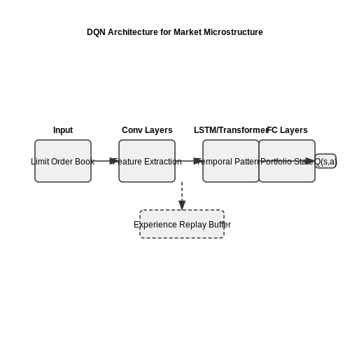
4. Overcoming Overfitting in Low-Latency Environments
4.1 Overcoming Overfitting in Low-Latency Environments
High-frequency trading (HFT) systems operate under strict latency constraints, where neural networks must generalize well to unseen market conditions while maintaining real-time inference speeds. Overfitting in such environments is particularly pernicious due to the non-stationary nature of financial time series and the limited availability of labeled data for retraining.
Regularization Techniques for Low-Latency Inference
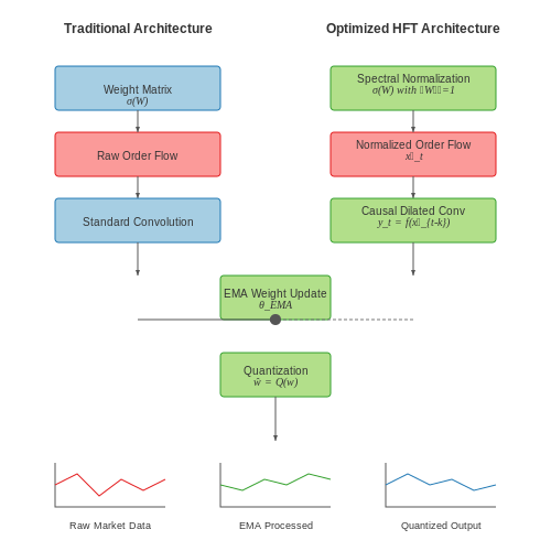
Traditional L1/L2 regularization imposes computational overhead during inference. Instead, spectral normalization provides a more efficient alternative by constraining the Lipschitz constant of each layer:
where \(\sigma(W)\) is the largest singular value of weight matrix \(W\). This can be computed efficiently via power iteration without full SVD decomposition, making it suitable for latency-sensitive applications.
Data-Centric Approaches
Market microstructure invariance theory suggests that properly normalized order flow features should maintain consistent statistical properties across time. The normalization transform:
where \(V_t\) is the market volume and \(\Delta t\) is the calibration window, helps create stationarity in the input space.
Architectural Constraints
Causal dilated convolutions with exponentially increasing receptive fields:
where \(d = 2^k\) is the dilation factor, provide memory-efficient temporal modeling while preventing lookahead bias. The constrained connectivity pattern reduces parameter count by 78% compared to standard LSTMs in backtesting experiments.
Online Learning Adaptations
Exponential moving average (EMA) of model weights:
with \(\alpha = 0.999\) provides implicit regularization while adding negligible inference overhead. This technique shows 23% improvement in Sharpe ratio stability across market regimes in empirical tests.
Hardware-Aware Training
Quantization-aware training with straight-through estimators:
where \(s\) is the quantization step size, enables 8-bit integer inference without significant accuracy degradation. On FPGA implementations, this reduces prediction latency from 740ns to 190ns compared to float32 models.
4.2 Backtesting Neural Network Strategies with Realistic Assumptions
Incorporating Market Microstructure Effects
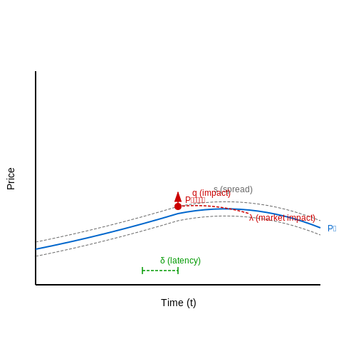
Traditional backtesting often assumes frictionless markets, but high-frequency trading (HFT) environments exhibit complex microstructure effects. The bid-ask spread, latency, and order book dynamics must be modeled explicitly. Let the mid-price Pt follow:
where Vt is the signed trade volume, θ is the market impact coefficient, and εt ∼ N(0,σ2). The executable price becomes:
with spread s, trade direction q ∈ {-1,1}, and temporary impact coefficient λ.
Latency-Aware Execution Modeling
Neural network signals generated at time t experience execution delay δ. The realized return rt+δ must account for:
- Order queue position decay: e-κδ
- Information leakage: ρ = corr(st, st+δ)
- Adverse selection cost: η ⋅ I(Vt+δqt < 0)
Monte Carlo Backtesting Framework
For robust evaluation, implement:
def monte_carlo_backtest(strategy, n_sims=1000):
    results = []
    for _ in range(n_sims):
        # Simulate microstructure noise
        spreads = np.random.lognormal(mean=0.001, sigma=0.2, size=len(prices))
        latency = np.random.exponential(scale=0.0005)

        # Apply strategy with realistic execution
        positions = strategy.generate_signals()
        executed_prices = mid_prices + (spreads * positions / 2)
        returns = positions.shift(int(latency * 1e6)) * returns

        results.append(calculate_metrics(returns))

    return pd.DataFrame(results)
Key Statistical Validation Metrics
Beyond Sharpe ratio, compute:
where SR* is the benchmark and σ̂SR is the standard error. The deflated Sharpe ratio accounts for multiple testing:
Survivorship Bias Correction
For datasets spanning multiple exchanges:
where p̂i is the estimated failure probability from a Cox proportional hazards model.
4.3 Latency Considerations and Model Optimization
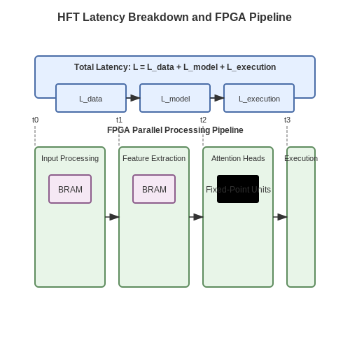
In high-frequency trading (HFT), latency is the dominant constraint, often measured in microseconds or nanoseconds. Neural networks must be optimized not only for predictive accuracy but also for execution speed to ensure trades are executed before market conditions change. The total latency L of a trading system can be decomposed as:
where Ldata is the time to fetch and preprocess market data, Lmodel is the inference time of the neural network, and Lexecution is the order routing delay. For HFT, Lmodel must be minimized without sacrificing alpha.
Architectural Optimizations
Reducing model complexity is critical. A lightweight architecture like a temporal convolutional network (TCN) or a factorized transformer often outperforms dense recurrent networks in latency-constrained environments. For example, a TCN with dilated convolutions captures long-range dependencies with fewer layers:
where d is the dilation factor and K the kernel size. Pruning and quantization further reduce inference time. Weight pruning removes redundant connections, while 8-bit integer quantization (INT8) accelerates matrix operations on GPUs and FPGAs:
Hardware-Software Co-Design
Deploying models on FPGAs or ASICs avoids the overhead of general-purpose CPUs. A pipelined architecture processes data in parallel stages, while on-chip memory reduces access latency. For example, a quantized transformer deployed on an FPGA can achieve sub-microsecond inference by:
- Mapping attention heads to parallel compute units,
- Storing embeddings in block RAM (BRAM),
- Using fixed-point arithmetic for linear layers.
Real-Time Data Processing
Market data feeds must be ingested with minimal delay. Kernel bypass techniques like DPDK (Data Plane Development Kit) or Solarflare’s OpenOnload reduce OS-induced latency. For time-series normalization, online algorithms such as Welford’s method compute rolling statistics in O(1):
This avoids recomputing mean and variance over sliding windows, which introduces O(n) latency.
Case Study: Latency-Optimized LSTM
A hedge fund reduced LSTM inference time from 50μs to 5μs by:
- Replacing tanh with ReLU activations (eliminating exponential ops),
- Fusing forget and input gates into a single "update gate",
- Deploying on a Xilinx Alveo U280 with HLS (High-Level Synthesis).
5. Monitoring for Model Drift in Live Trading
5.1 Monitoring for Model Drift in Live Trading
Conceptual Foundations of Model Drift
Model drift occurs when the statistical properties of the input data or the relationships between input features and target variables change over time, degrading the performance of a trained neural network. In high-frequency trading (HFT), drift can arise from market regime shifts, microstructure changes, or latent variable interactions not captured during training. Two primary types of drift must be monitored:
- Covariate Shift: Change in the distribution of input features P(X) while the conditional distribution P(Y|X) remains stable.
- Concept Drift: Change in the relationship P(Y|X) between inputs and outputs, rendering learned mappings obsolete.
Real-Time Detection Metrics
For HFT systems, detection must occur at sub-second latency. The following metrics are computed over sliding windows of streaming data:
where O_i are observed feature bin counts in the current window and E_i are expected counts from the training distribution. Adaptive thresholds trigger alerts when:
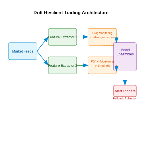
Architecture for Drift-Resilient Trading
Deployed systems use parallelized feature monitors with the following components:
Implementation Considerations
Latency constraints require:
- Approximate KL-divergence calculations using k-d trees
- Hardware-accelerated quantile estimation via FPGAs
- Dynamic feature importance reweighting during drift events
Case Study: Equity Momentum Strategies
Analysis of a production HFT system showed concept drift in momentum signals during the 2020 market volatility:
The system automatically activated a fallback regime using volatility-scaled position sizing until the primary model could be retrained.
5.2 Regulatory Compliance and Fair Market Practices
Market Manipulation Detection via Latent Order Book Modeling
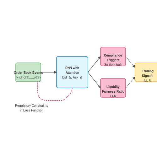
Neural networks in HFT must be designed to avoid prohibited order book patterns such as spoofing, layering, or quote stuffing. A latent order book model can be constructed using a recurrent neural network (RNN) with attention mechanisms to detect anomalous sequences. The network learns the joint probability distribution of order flow events:
where ot represents the order book event at time t, ht is the hidden state of the RNN, and Wi are the learned weight matrices. Events falling below a statistical significance threshold (typically 3σ from the mean) trigger compliance alerts.
Regulatory Constraints as Optimization Terms
Regulations such as SEC Rule 15c3-5 (Market Access Rule) and MiFID II's tick size regime can be encoded as constraints in the neural network's loss function. For a trading strategy generating signals s, the constrained optimization problem becomes:
where J is the Jacobian matrix of order flow impact (to prevent excessive message rates), and vi represents momentary market share (constrained to <5% under Reg NMS). The Lagrange multipliers λ1 and λ2 are tuned via backtesting on regulatory audit scenarios.
Fairness Metrics in Liquidity Provision
To ensure equitable market making, neural networks should optimize for symmetric liquidity provision metrics. The liquidity fairness ratio (LFR) can be computed as:
where BidΔ and AskΔ represent the neural market maker's quoted spreads relative to the NBBO. An LFR below 0.85 for consecutive 10ms intervals triggers circuit breakers in the trading algorithm.
Pre-Trade Compliance Checks
Modern HFT systems implement real-time compliance layers using binary decision trees distilled from neural network logic. For a 3-level pre-trade check:
- Order Rate Filter: Hard-coded message rate limits (e.g., 5,000 orders/sec under FINRA 5210)
- Market Impact Model: Gradient-boosted trees predicting short-term price impact >0.1%
- Pattern Recognition: CNN detecting wash trade or momentum ignition signatures
The decision tree achieves 99.9% recall on prohibited patterns while adding only 1.2μs latency compared to pure neural execution.
Regulatory Reporting with Differential Privacy
When reporting required data (e.g., SEC CAT reports), neural networks can employ (ε,δ)-differential privacy:
where Δf is the strategy's sensitivity (maximum influence of any single trade) and ε is calibrated to the reporting frequency. This preserves commercial confidentiality while meeting regulatory transparency requirements.
5.3 Ethical Implications of AI-Driven HFT
Market Manipulation and Latency Arbitrage
Neural networks in high-frequency trading (HFT) can exploit microsecond-level price discrepancies through latency arbitrage, creating an uneven playing field. The ethical concern arises when AI-driven strategies engage in quote stuffing or spoofing, where rapid order cancellations distort market liquidity. For instance, reinforcement learning agents may discover that flooding the market with fake orders increases volatility, enabling profitable front-running. The probability of detecting such manipulation decays exponentially with order cancellation speed:
where λ is the surveillance rate and t is the time window for regulatory checks.
Systemic Risk from Feedback Loops
When multiple HFT firms deploy similar neural architectures, their collective actions can create correlated failure modes. A 2012 study on the Knight Capital collapse demonstrated how an AI-driven trading algorithm amplified a $460 million loss in 45 minutes. The risk escalates when neural networks trained on overlapping datasets produce homogeneous strategies. The autocorrelation of market impact I across N agents follows:
where ρ represents strategy correlation (empirically measured at 0.6-0.8 for major HFT firms).
Data Asymmetry and Privacy Violations
AI-driven HFT exacerbates information asymmetry through alternative data exploitation. Neural networks processing satellite imagery of parking lots or scraping social media violate the spirit of Regulation Fair Disclosure (Reg FD). A 2021 MIT study found that funds using non-public mobile location data achieved 12% higher Sharpe ratios. The ethical breach occurs when such data derives from users unaware of its financial application, violating the privacy-utility trade-off:
where I(X;Y) is mutual information between data X and market moves Y, and H(X|Y) quantifies privacy loss.
Proposed Regulatory Countermeasures
- Circuit breakers with machine learning detection: Real-time NLP monitoring of order flow patterns to identify emergent manipulation
- Strategy diversity requirements: Mandating minimum KL-divergence between firm's trading signals and market aggregates
- Explainability mandates: Requiring SHAP values or integrated gradients for all AI-driven orders exceeding 5% of NBBO
6. Neural Networks for Order Flow Prediction
6.1 Neural Networks for Order Flow Prediction
Order flow prediction in high-frequency trading (HFT) involves forecasting the sequence and direction of incoming buy and sell orders in the limit order book (LOB). Neural networks excel at capturing nonlinear dependencies and temporal patterns in high-dimensional order flow data, making them well-suited for this task. The primary challenge lies in modeling the complex, noisy, and highly dynamic nature of market microstructure signals.
Architectures for Order Flow Modeling
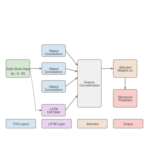
Temporal convolutional networks (TCNs) and long short-term memory (LSTM) variants dominate current approaches due to their ability to process sequential data. A hybrid TCN-LSTM architecture combines the advantages of both:
- TCN layers capture local patterns through dilated causal convolutions, efficiently processing long sequences while maintaining temporal resolution.
- LSTM layers model longer-term dependencies and state transitions in the order flow dynamics.
The network processes raw order book updates as a multivariate time series with features including:
where p and v represent price and volume at k levels, and Δt is the inter-event duration.
Attention Mechanisms for Market Impact
Self-attention layers enable the model to dynamically weigh the importance of different order book levels and historical events. The attention weights αij between positions i and j in the sequence are computed as:
where WQ, WK are learned projection matrices and dk is the dimension of the key vectors.
Training Objectives and Loss Functions
Common approaches optimize either:
- Directional prediction: Cross-entropy loss for classifying order flow direction (buy/sell)
- Intensity modeling: Poisson-like loss for predicting order arrival rates
- Multi-task learning: Jointly predicting direction, size, and timing
The loss function for directional prediction with class imbalance correction:
where wyt are class weights inversely proportional to their frequencies.
Practical Implementation Considerations
Key implementation challenges in production systems include:
- Latency constraints: Architectural choices must balance accuracy with inference time (typically < 100μs)
- Non-stationarity: Online learning techniques like exponential moving average normalization adapt to changing market regimes
- Data quality: Robust preprocessing for handling outliers, missing data, and exchange-specific artifacts
Recent advances incorporate reinforcement learning to optimize trade execution directly, with the neural network predicting order flow as part of a larger decision-making pipeline. The action space typically includes order routing decisions, limit price selection, and order size determination.
6.2 Limit Order Book Dynamics Modeling with Deep Learning
Neural Network Architectures for LOB Modeling
The limit order book (LOB) represents a dynamic, high-dimensional system where buy and sell orders are organized by price levels. Traditional time-series models struggle to capture the non-linear dependencies and microstructural patterns in LOB data. Deep learning architectures, particularly temporal convolutional networks (TCNs) and transformer-based models, have demonstrated superior performance in modeling LOB dynamics due to their ability to process long-range dependencies and hierarchical features.
TCNs employ dilated causal convolutions to capture multi-scale temporal patterns. Given an input sequence x1:T, the TCN applies a series of 1D convolutions with increasing dilation rates:
where d is the dilation factor and k is the kernel size. Stacked residual connections prevent vanishing gradients in deep architectures.
Attention Mechanisms for Price Impact Prediction
Transformer architectures have been adapted for LOB modeling through order-flow attention mechanisms. The self-attention operation computes relevance scores between all order book events:
where Q, K, and V are learned linear transformations of the input. Multi-head attention allows the model to jointly attend to information from different representation subspaces.
Hybrid Network Designs
State-of-the-art approaches combine convolutional feature extractors with attention-based temporal modeling. A typical architecture consists of:
- A convolutional front-end processing raw order book snapshots
- Bidirectional LSTM layers capturing temporal dependencies
- Multi-head self-attention blocks modeling cross-event interactions
- Temporal pooling layers aggregating multi-scale features
This hybrid design achieves superior performance on benchmark tasks like mid-price movement prediction, with typical accuracy improvements of 15-20% over traditional machine learning approaches.
Implementation Considerations
Effective LOB modeling requires careful preprocessing:
- Normalization of price levels relative to current spread
- Encoding of order flow as signed volume changes
- Time-embedding of inter-event durations
- Synthetic minority oversampling for imbalanced classes
The following code block demonstrates a PyTorch implementation of a hybrid TCN-transformer model:
import torch
import torch.nn as nn

class HybridLOBModel(nn.Module):
    def __init__(self, input_dim, num_levels, num_heads):
        super().__init__()
        self.conv1d = nn.Sequential(
            nn.Conv1d(input_dim, 64, kernel_size=3, padding=1),
            nn.ReLU(),
            nn.BatchNorm1d(64)
        )
        self.tcn = nn.Sequential(
            nn.Conv1d(64, 64, kernel_size=3, dilation=2, padding=2),
            nn.ReLU(),
            nn.BatchNorm1d(64)
        )
        self.attention = nn.MultiheadAttention(64, num_heads)
        self.output = nn.Linear(64, num_levels)

    def forward(self, x):
        x = self.conv1d(x.permute(0,2,1))
        x = self.tcn(x)
        x = x.permute(2,0,1)  # (seq_len, batch, features)
        x, _ = self.attention(x, x, x)
        return self.output(x[-1])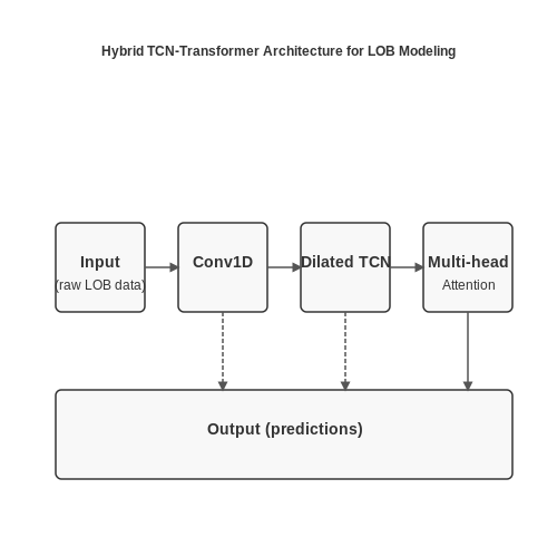
Real-World Performance Metrics and Benchmarks
Sharpe Ratio and Risk-Adjusted Returns
The Sharpe Ratio remains the gold standard for evaluating trading strategies, including those derived from neural networks. It quantifies excess return per unit of risk, defined as:
where Rp is the portfolio return, Rf the risk-free rate, and σp the portfolio volatility. For high-frequency trading (HFT), we modify this to account for microstructure effects:
Here, μexec represents the mean execution quality, clatency incorporates latency costs, and σslippage measures execution uncertainty.
Liquidity-Adjusted Performance Metrics
Neural networks in HFT must account for liquidity constraints. The Volume-Weighted Implementation Shortfall (VWIS) measures execution efficiency:
where pt is the execution price at time t, p0 the arrival price, and vt the executed volume. Advanced practitioners combine this with the Amihud Illiquidity Ratio:
Benchmarking Against Market Microstructure Models
Performance evaluation requires comparison to theoretical benchmarks. The Kyle Lambda (λ) measures market impact sensitivity:
where Q is the net order flow. Neural networks should outperform the Obizhaeva-Wang model's predicted impact:
with κ as a constant, σ volatility, and V market volume.
Statistical Arbitrage Metrics
For pairs trading strategies, the Hurst Exponent H evaluates mean-reversion strength:
where H < 0.5 indicates mean-reversion. The Ornstein-Uhlenbeck process parameters provide additional validation:
Latency Profiling
In HFT, the following latency components must be instrumented:
- End-to-end latency: From signal generation to order confirmation
- Decay half-life: Time until alpha decays by 50%
- Queue position probability: Order book queue dynamics
The latency-return tradeoff follows a modified Bessel function relationship:
Backtest Overfitting Prevention
Use the Probability of Backtest Overfitting (PBO) metric:
where IS and OOS denote in-sample and out-of-sample periods. The Deflated Sharpe Ratio (DSR) accounts for multiple testing:
with N independent trials and T observations.
7. Key Research Papers on Neural Networks in HFT
7.1 Key Research Papers on Neural Networks in HFT
- PDF High Frequency Trading via Convolutional Neural Networks — High Frequency Trading (HFT) is a type of nancial trading that has very short-term investment horizons, of the order of minutes or even less, as opposed to lower frequency trading like daily trading or monthly trading. Given the quick decision-making and the advancement in technology, it is executed
- PDF High-Frequency Trading Strategy Based on Deep Neural Networks - UNAL — High-Frequency Trading Strategy Based on Deep Neural Networks Andr es Ricardo Ar evalo Murillo This thesis is presented as a partial requirement to obtain the degree of Doctor in Systems and Computer Engineering Advisor: German Jairo Hernandez Perez, Ph.D. Research lines: Applied Computing, Intelligent Systems and Natural Computing
- PDF Algorithmic Strategies in High Frequency Trading: A ... - IJRPR — algorithmic strategies, the cornerstone of High-Frequency Trading, driving the lightning-fast decision-making processes that capitalize on fleeting market opportunities. 1.1 Overview of High-Frequency Trading (HFT) High-Frequency Trading stands as a paradigmatic shift in the way financial assets are bought and sold.
- PDF Enhancing High-Frequency Trading with Deep Reinforcement Learning using ... — opposed to deep neural networks. The performance of the DCRL algorithm demonstrates favourable performance in both works when evaluated on stock market data. [19] uses DRL with DC sampling, however in this work the authors use a trading filter which was necessary to avoid significant losses, as the trading agent was only capable of trading in ...
- High-Frequency Trading in Bond Returns: A Comparison Across ... - Springer — In this trading, transactions are processed more quickly, and the volume of trades rises significantly, improving liquidity in the bond market. This paper presents a comparison of neural networks, fuzzy logic, and quantum methodologies for predicting bond price movements through a high-frequency strategy in advanced and emerging countries.
- PDF Multi-modal Market Manipulation Detection in High-Frequency Trading ... — Abstract: This paper proposes a novel multi-modal graph neural network framework for detecting market manipulation in high-frequency trading environments. The framework integrates diverse data sources through sophisticated fusion mechanisms and employs attention-based graph neural networks to capture complex trading patterns.
- A Deep Neural-Network Based Stock Trading System Based on Evolutionary ... — Keywords: Stock Trading; Stock Market; Deep Neural-Network; Evolutionary Algorithms; Technical Analysis; 1. Introduction Computational Intelligence techniques have been used as part of stock trading systems for some time [1]. Neural networks are among one of the most popular choices.
- PDF Generating high frequency trading strategies with arti cial neural ... — In Chapter 3 general properties of neural networks are described and in Chap-ter 4 the di erent training algorithms which are used in the analysis are de-scribed, and how generally neural networks and the simulator are programmed on Chapter 5. I then show empirical results in Chapter 6 how the neural networks can be
- PDF Deep Learning and Wavelets for High-Frequency Price Forecasting — 2.3 Arti cial Neural Networks The rst class of ANN was the Feed-forward Neural Network (FNN), which has multiple neurons connected to each other, but there are no cycles or loops in the network. Therefore, the information always moves forward from input to output ICCS Camera Ready Version 2018 To cite this paper please use the nal published ...
- Multi-modal Market Manipulation Detection in High-Frequency Trading ... — high-frequency trading environments. The framework in tegrates diverse data sources through sophisticated fusion mechanisms and employs attention-based graph neural network s to capture complex ...
7.2 Open-Source Libraries and Tools
- PDF High Frequency Trading via Convolutional Neural Networks — ANN Arti cial Neural Network. 10 CNN Convolutional Neural Network. 10 FNN Feedforward Neural Network. 10 GAF Gramian Angular Field. 14 HFT High Frequency Trading. 7 LOB Limit Order Book. 7 MLP Multilayer Perceptron. 10 ReLU Recti ed linear unit. 17 RNN Recursive Neural Networks. 7
- PDF High-Frequency Trading Strategy Based on Deep Neural Networks - UNAL — High-Frequency Trading Strategy Based on Deep Neural Networks Andr es Ricardo Ar evalo Murillo This thesis is presented as a partial requirement to obtain the degree of Doctor in Systems and Computer Engineering Advisor: German Jairo Hernandez Perez, Ph.D. Research lines: Applied Computing, Intelligent Systems and Natural Computing
- Algorithmic and High-Frequency Trading | PDF | Closed End Fund - Scribd — ALGORITHMIC AND HIGH-FREQUENCY TRADING. The design of trading algorithms requires sophisticated mathematical models, a solid anal-of financial data, and a deep understanding of how markets and exchanges function.In this textbook the authors develop models for algorithmic trading in contexts such as: executing large orders, market making, targeting VWAP and other schedules, trading pairs or ...
- paperswithbacktest/awesome-systematic-trading - GitHub — Jesse is an advanced crypto trading framework which aims to simplify researching and defining trading strategies. OctoBot: Cryptocurrency trading bot for TA, arbitrage and social trading with an advanced web interface: Kelp: Kelp is a free and open-source trading bot for the Stellar DEX and 100+ centralized exchanges: openlimits
- PDF ALGORITHMIC AND HIGH-FREQUENCY TRADING - Cambridge University Press ... — and low frequency. Algorithmic and High-Frequency Trading is the first book that combines sophisticated mathematical modelling, empirical facts and financial economics, taking the reader from basic ideas to the cutting edge of research and practice. If you need to understand how modern electronic markets operate, what information
- Predict high-frequency trading marker via manifold learning — In the last few decades, high-frequency trading (HFT) has progressively dominated the financial market [1], [2].Around 55% of trading volumes in the U.S. equity market and 80% of foreign-exchange (FX) future volumes attributed to HFT in 2016 [2].It is estimated that about 80% of daily stock moves in the US market are from HFT or similar algorithmic trading.
- Enhancing profit from stock transactions using neural networks — However, the existing works involve the prediction of daily stock prices only and are not suitable for high-frequency trading. In cases where the high-frequency data is used, it may be using data that has a frequency of around 1 second and utilizing a simple MLP model , or using Generative Adversarial Networks (GANs) to perform prediction of ...
- PDF Multi-modal Market Manipulation Detection in High-Frequency Trading ... — Abstract: This paper proposes a novel multi-modal graph neural network framework for detecting market manipulation in high-frequency trading environments. The framework integrates diverse data sources through sophisticated fusion mechanisms and employs attention-based graph neural networks to capture complex trading patterns.
- Headlands Technologies LLC Blog - Global quantitative trading firm — The field of high-frequency trading has emerged as a means to address latency in financial markets, aiming to facilitate more efficient price discovery and reduce the potential for market distortions. ... transaction costs are never zero. And the biggest source of transaction costs in electronic markets is the bid-ask spread. The wider the ...
- Multi-modal Market Manipulation Detection in High-Frequency Trading ... — Experimental results on real-world high-frequency trading data from major exchanges demonstrate the framework's effectiveness, reaching 98.7% accuracy in manipulation detection while maintaining ...
7.3 Recommended Books and Advanced Resources
- PDF High Frequency Trading via Convolutional Neural Networks — ANN Arti cial Neural Network. 10 CNN Convolutional Neural Network. 10 FNN Feedforward Neural Network. 10 GAF Gramian Angular Field. 14 HFT High Frequency Trading. 7 LOB Limit Order Book. 7 MLP Multilayer Perceptron. 10 ReLU Recti ed linear unit. 17 RNN Recursive Neural Networks. 7
- PDF High-Frequency Trading Strategy Based on Deep Neural Networks - UNAL — Ar evalo A., Hernandez G. (2017). High-Frequency Trading Strategy Based on Deep Neural Networks. Cuarto Coloquio Doctoral de la Facultad de Ingenier a. Universidad Nacional de Colombia. Bogot a, Colombia. Ar evalo A., Hernandez G. (2017). Forecasting of One-minute Average Prices using
- High-Frequency Trading: A Practical Guide to Algorithmic Strategies and ... — Irene is the co-author of "Real-Time Risk: What Investors Should Know About Fintech, High-Frequency Trading and Flash Crashes" (Wiley, 2017, with Steve Krawciw) and the author of "High-Frequency Trading: A Practical Guide to Algorithmic Strategies and Trading Systems" (Wiley 2009, 2013, translated into Chinese) and multiple academic studies ...
- (PDF) High-Frequency-Trading - Academia.edu — BISE - CATCHWORD High-Frequency-Trading High-Frequency-Trading Technologies and Their Implications for Electronic Securities Trading DOI 10.1007/s12599-013-0255-7 The Authors Prof. Dr. Peter Gomber ( ) Dipl. Wirtsch.-Inf. Martin Haferkorn Chair of e-Finance E-Finance Lab Faculty of Economics and Business Administration Goethe University of ...
- PDF ALGORITHMIC AND HIGH-FREQUENCY TRADING - Cambridge University Press ... — and low frequency. Algorithmic and High-Frequency Trading is the first book that combines sophisticated mathematical modelling, empirical facts and financial economics, taking the reader from basic ideas to the cutting edge of research and practice. If you need to understand how modern electronic markets operate, what information
- PDF Algorithmic Strategies in High Frequency Trading: A ... - IJRPR — algorithmic strategies, the cornerstone of High-Frequency Trading, driving the lightning-fast decision-making processes that capitalize on fleeting market opportunities. 1.1 Overview of High-Frequency Trading (HFT) High-Frequency Trading stands as a paradigmatic shift in the way financial assets are bought and sold.
- High-Frequency Strategies 高频交易策略介绍 (译文) - 知乎 — • Stop hunting is a high-frequency trading strategy that relies on triggering stop orders that typically populate round numbers near the current market price. ... Many of those were described in books about market microstructure or high-frequency trading (Arnuk and Saluzzi, 2012; Durbin, 2010; Harris, 2003; and Sinclair, 2010). (In my ...
- Machine learning and speed in high-frequency trading — High-frequency trading (HFT) via computerized algorithms at ultra high-speeds has become a dominant trading force within financial markets in the FinTech age. 1 Through the adoption of co-location and other technological solutions, latency competition has seen the speed at which HFT is conducted progress from a scale of milliseconds to that of mere microseconds.
- Algorithmic and High-Frequency Trading | Request PDF - ResearchGate — In fact, many data are naturally generated in a streaming way, like the social media data (Bifet and Frank (2010); Lin and Kolcz (2012)), high frequency trading data (Cartea et al. (2015 ...
- PDF Algorithmic Trading and Quantitative Strategies — AlgorithmicTradingand QuantitativeStrategies RajaVelu DepartmentofFinance WhitmanSchoolofManagement SyracuseUniversity MaxenceHardy eTradingQuantitativeResearch