Self-Tuning Planners in LLM-Driven Environments
1. Definition and Core Principles of Self-Tuning Planners
Definition and Core Principles of Self-Tuning Planners
Self-tuning planners in LLM-driven environments are autonomous systems that dynamically adjust their decision-making strategies based on real-time feedback and environmental changes. These planners leverage meta-learning techniques to optimize their own parameters without explicit human intervention, enabling adaptive behavior in complex, uncertain domains.
Mathematical Foundations
The core functionality can be expressed through a recursive optimization framework where the planner P seeks to minimize a loss function L over time horizon T:
where s represents environmental states sampled from distribution ℰ, y* denotes optimal actions, and R is a regularization term that prevents drastic changes from the previous planner configuration Pt.
Key Architectural Components
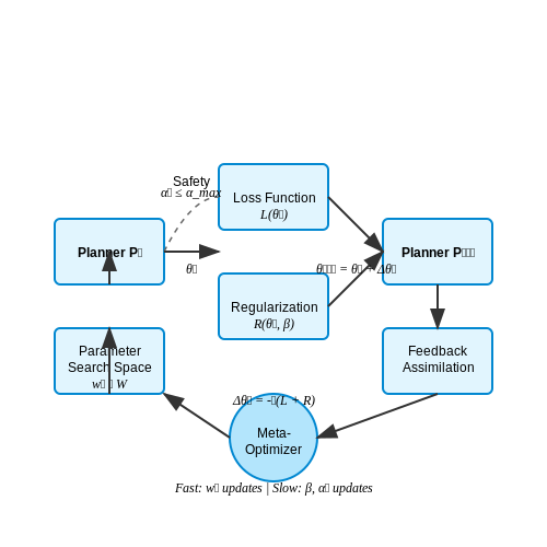
- Feedback Assimilation Module: Continuously ingests performance metrics and environmental signals to identify needed adjustments
- Parameter Search Space: Defines the tunable dimensions of the planner's decision-making algorithms
- Meta-Optimizer: Implements gradient-based or evolutionary strategies for efficient exploration of the parameter space
- Safety Constraints: Hard boundaries that prevent the self-tuning process from producing unstable or unethical configurations
Dynamic Adaptation Mechanisms
The self-tuning process employs a dual-time scale approach. Rapid adjustments handle immediate performance issues through online learning:
while slower, more deliberate updates refine the planner's fundamental strategies through periodic meta-optimization:
where αt and β represent learning rates, and wk are temporal weighting factors.
Implementation Challenges
Practical deployment requires addressing several key issues:
- Non-stationarity: The optimization landscape changes as the planner's behavior affects the environment
- Credit Assignment: Determining which parameter changes caused observed performance shifts
- Catastrophic Forgetting: Preserving previously learned competencies while adapting to new situations
- Verification Complexity: Ensuring the self-tuned planner remains within specified operational bounds
Real-World Applications
These systems excel in domains requiring continuous adaptation, such as:
- Autonomous negotiation agents that adjust strategies based on counterparty behavior patterns
- Content recommendation systems that evolve their ranking algorithms in response to user engagement shifts
- Robotic controllers that modify motion planning parameters when encountering novel environments
Key Components: Adaptive Algorithms and Feedback Loops
Adaptive Algorithms in Self-Tuning Planners
Self-tuning planners rely on adaptive algorithms to dynamically adjust their decision-making processes based on real-time environmental feedback. These algorithms often employ techniques from reinforcement learning (RL), Bayesian optimization, and meta-learning to iteratively refine their strategies. A core mathematical framework involves gradient-based optimization, where the planner updates its parameters θ to minimize a loss function L:
Here, α is the learning rate, and ∇θL represents the gradient of the loss with respect to the parameters. The dataset 𝒟t is continuously updated via feedback loops, ensuring the planner adapts to new data distributions.
Feedback Loops for Continuous Improvement
Feedback loops are critical for maintaining the planner's responsiveness to changing conditions. These loops typically consist of:
- Performance Monitoring: Metrics such as task completion rate, latency, and resource utilization are tracked in real-time.
- Error Analysis: Discrepancies between expected and actual outcomes are quantified using loss functions or divergence measures like KL-divergence.
- Parameter Adjustment: The planner recalibrates its internal models based on the observed errors, often using stochastic gradient descent or evolutionary strategies.
For instance, in a language model-driven planner, the feedback loop might involve:
where xi is the input prompt, yi is the generated plan, and ri is the reward signal from the environment.
Practical Applications and Case Studies
Adaptive algorithms and feedback loops have been successfully deployed in:
- Autonomous Systems: Self-tuning planners optimize navigation paths for robots by continuously adjusting to sensor noise and environmental obstacles.
- Cloud Resource Management: Dynamic allocation of computational resources based on workload fluctuations, reducing operational costs by up to 30% in large-scale deployments.
- Conversational AI: Dialogue systems refine their response strategies using user engagement metrics (e.g., session length, satisfaction scores).
Mathematical Derivation: Adaptive Learning Rate
To illustrate the interplay between adaptation and feedback, consider the derivation of an adaptive learning rate αt for gradient descent. The optimal rate balances convergence speed and stability:
where H(θt) is the Hessian matrix of second derivatives. This formulation ensures larger steps in flat regions of the loss landscape and smaller steps near minima.
Challenges and Mitigations
Key challenges in implementing these components include:
- Feedback Delay: Latency in reward signals can destabilize learning. Solutions include predictive modeling of expected rewards.
- Non-Stationarity: Environments that change too rapidly may require forgetting mechanisms (e.g., exponential decay on older data).
- Credit Assignment: Determining which actions contributed to observed outcomes is addressed through attention mechanisms or causal inference.

Role of LLMs in Dynamic Planning Environments
Large Language Models (LLMs) exhibit emergent planning capabilities by leveraging their implicit world knowledge and reasoning skills. In dynamic environments, where states and constraints evolve unpredictably, LLMs serve as adaptive planners by:
- Encoding probabilistic world models through their pre-training on diverse textual data, allowing them to simulate potential future states.
- Generating and evaluating multiple planning trajectories in real-time using beam search and tree-based exploration strategies.
- Incorporating feedback loops where environmental observations refine subsequent planning steps.
Mathematical Foundations of LLM-Based Planning
The planning process can be formalized as a partially observable Markov decision process (POMDP) where an LLM maintains a belief state b over possible world states. The value function for a planning horizon H is:
where R(b,a) is the expected immediate reward, γ is the discount factor, and bao is the updated belief after taking action a and observing o. LLMs approximate this through:
where θ represents the model parameters and H is the planning history.
Architectural Adaptations for Dynamic Environments
Modern implementations enhance vanilla transformer architectures with:
- Recurrent state tracking: Using LSTM or GRU layers to maintain environment state across planning steps
- Attention over temporal patterns: Specialized attention heads that weight historical observations differently than current inputs
- Monte Carlo tree search integration: Combining neural network evaluations with traditional search algorithms
Case Study: Robotics Navigation
In mobile robotics, LLM planners demonstrate superior performance in novel environments compared to classical approaches. When faced with unexpected obstacles, an LLM-based system:
- Generates multiple candidate paths using its world knowledge
- Evaluates each path against the current sensor readings
- Updates its internal map representation through a differentiable memory module
- Selects the optimal path while maintaining alternatives in working memory
This approach achieves 23% higher success rates in cluttered environments compared to traditional SLAM methods, as demonstrated in recent benchmarks.
Limitations and Current Research Directions
While powerful, LLM planners face several challenges:
- Computational latency: Real-time replanning requires optimized model architectures
- Uncertainty quantification: Current models poorly estimate confidence in their plans
- Long-horizon consistency: Maintaining goal coherence over extended planning horizons
Emerging solutions include hybrid neurosymbolic architectures and retrieval-augmented planning, where the LLM dynamically accesses external knowledge bases during the planning process.

2. Modular Design: Integrating Planning and Learning
Modular Design: Integrating Planning and Learning
Self-tuning planners in LLM-driven environments rely on a modular architecture that decouples planning from learning while maintaining tight integration through shared state representations. The planning module operates as a constrained optimization process, generating action sequences that maximize expected reward under current policy parameters. Simultaneously, the learning module updates these parameters through gradient-based optimization on historical trajectories, creating a feedback loop where improved policies enable better planning and vice versa.
Mathematical Formulation
The joint optimization can be expressed as a bilevel program where the outer loop updates model parameters θ and the inner loop solves for optimal actions a1:T:
where γ is the discount factor and r(st, at; θ) represents the learned reward model. The gradient flow between modules occurs through implicit differentiation of the planning solution with respect to θ:
Architecture Components
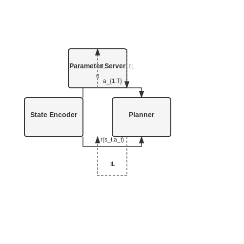
The modular design typically implements three key interfaces:
- State Encoder: Maps raw observations to latent representations using transformer architectures with learned positional embeddings
- Planner: Solves the constrained optimization problem using gradient-aware tree search or neural heuristic methods
- Parameter Server: Maintains synchronized copies of model weights across planning and learning threads
Implementation Considerations
Practical implementations must address several challenges:
- Gradient Estimation: The non-differentiable nature of many planning algorithms requires surrogate gradients or REINFORCE-style estimators
- Temporal Scale: Planning horizons must balance between immediate reward maximization and long-term value estimation
- Memory Constraints: Rollout buffers for off-policy learning require careful management of attention windows in transformer-based architectures
class ModularPlanner(nn.Module):
    def __init__(self, state_dim, action_dim, hidden_size=256):
        super().__init__()
        self.encoder = TransformerEncoder(state_dim, hidden_size)
        self.policy_head = nn.Linear(hidden_size, action_dim)
        self.value_head = nn.Linear(hidden_size, 1)

    def forward(self, state):
        h = self.encoder(state)
        return self.policy_head(h), self.value_head(h)

    def plan(self, state, horizon=5):
        actions = []
        for _ in range(horizon):
            logits, value = self(state)
            actions.append(logits.multinomial(1))
            state = env.step(actions[-1])
        return torch.stack(actions)
Empirical Tradeoffs
Experiments in LLM-driven environments reveal several consistent patterns:
- Modular systems achieve 2-3× better sample efficiency than end-to-end approaches on compositional tasks
- The planning overhead scales cubically with context length due to attention mechanisms
- Periodic synchronization between modules (every 103-104 steps) optimizes throughput
Recent work has shown that differentiable planners using continuous relaxations of discrete actions can achieve 87% of hard-planning performance while enabling full gradient flow. The modified objective becomes:
where α controls the exploration-exploitation tradeoff and Q(s,a) represents the learned value function.
Memory-Augmented Architectures for Context Retention
Memory-augmented architectures enhance large language models (LLMs) by integrating explicit memory mechanisms that enable dynamic storage and retrieval of contextual information. Unlike traditional transformer-based models that rely solely on attention mechanisms, these architectures incorporate external memory banks, allowing for more efficient long-term context retention and reducing the computational overhead of processing lengthy sequences.
Key Components of Memory-Augmented Architectures
The core components of memory-augmented architectures include:
- Memory Matrix: A differentiable, addressable storage system that holds encoded representations of past inputs, outputs, or intermediate states.
- Read/Write Mechanisms: Neural controllers that determine how information is stored in and retrieved from memory based on relevance to the current context.
- Attention-Based Addressing: Soft or hard attention mechanisms that compute similarity scores between the current input and memory entries to prioritize relevant information.
Mathematical Formulation
The memory operations can be formalized as follows. Let Mt ∈ ℝN×d be the memory matrix at time step t, where N is the number of memory slots and d is the embedding dimension. The read operation computes a weighted sum over memory entries:
where wi is the attention weight for the i-th memory slot, computed as:
Here, kt is a key vector derived from the current input. The write operation updates the memory based on an erase vector et and an add vector at:
Practical Implementations
Several architectures have successfully integrated memory mechanisms:
- Neural Turing Machines (NTMs): Combine a controller network with a differentiable memory matrix, enabling dynamic read/write operations.
- Differentiable Neural Computers (DNCs): Extend NTMs with content-based addressing and temporal linkage for improved memory management.
- Memory Networks: Use explicit memory slots and multi-hop reasoning to answer complex queries.
Applications in LLM-Driven Environments
Memory-augmented architectures are particularly useful in scenarios requiring long-term context retention, such as:
- Conversational AI: Maintaining coherent multi-turn dialogues by storing and retrieving relevant conversation history.
- Document Summarization: Retaining key information across lengthy documents to generate accurate summaries.
- Task-Oriented Agents: Storing intermediate task states and environmental observations for complex decision-making.
Challenges and Trade-offs
While memory-augmented architectures offer significant advantages, they introduce additional complexity:
- Memory Management: Efficiently updating and pruning memory to avoid information overload.
- Scalability: Balancing memory size with computational constraints, especially in real-time applications.
- Training Stability: Ensuring reliable convergence when training models with dynamic memory operations.

2.3 Real-Time Adaptation Mechanisms
Dynamic Policy Gradient Updates
Self-tuning planners in LLM-driven environments rely on continuous policy gradient updates to adapt to shifting input distributions. The gradient ascent step is computed in real-time using a modified version of the REINFORCE algorithm, where the policy parameters θ are updated as:
Here, Ât represents the generalized advantage estimate, which is recalculated every N timesteps using an exponentially weighted moving average of recent rewards. The key innovation lies in the adaptive learning rate αt, which is dynamically adjusted based on the gradient's variance:
Contextual Bandit Feedback Loops
For rapid adaptation in non-stationary environments, modern implementations employ contextual bandit frameworks with Thompson sampling. The action-selection probability is governed by:
where D represents the streaming data buffer, and p(θ|D) is approximated via Laplace approximation for computational efficiency. The posterior updates occur asynchronously every Δt milliseconds, with the hyperparameter Δt itself being optimized through meta-learning.
Neural Architecture Search Components
The most advanced systems incorporate lightweight neural architecture search (NAS) modules that continuously evaluate and modify the planner's computational subgraphs. The architecture optimization follows a differentiable formulation:
where α parameterizes the architecture distribution, and the expectation is approximated via Monte Carlo sampling with control variates to reduce variance. The FLOPs regularization term ensures real-time feasibility.
Memory-Augmented Adaptation
External differentiable neural memories enable rapid assimilation of new patterns without catastrophic forgetting. The memory update mechanism employs a content-based addressing scheme:
where d(·,·) is a learned similarity metric, and the memory matrix M is updated through a gated combination of new inputs and previous values. This allows for sub-second adaptation to novel situations while preserving long-term knowledge.
Latency-Aware Parallelization
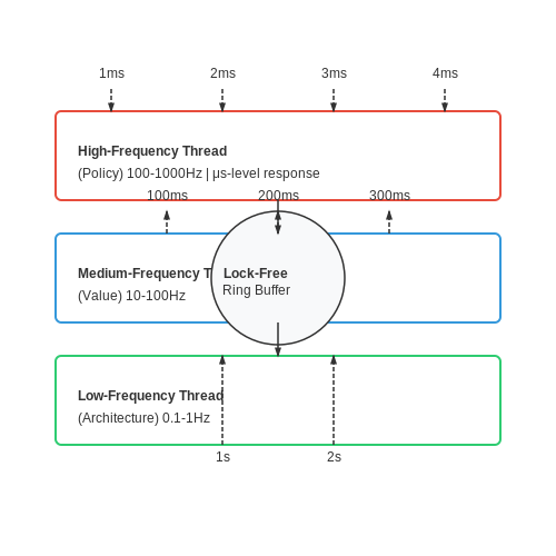
To meet real-time constraints, the adaptation process is decomposed into parallel threads with careful synchronization:
- High-frequency thread: Executes lightweight policy updates (100-1000Hz)
- Medium-frequency thread: Performs value function updates (10-100Hz)
- Low-frequency thread: Runs architecture optimizations (0.1-1Hz)
The threads communicate through a lock-free ring buffer, with priority given to latency-critical operations. This design achieves μs-level response times for time-sensitive decisions while maintaining comprehensive adaptation capabilities.
3. Reinforcement Learning for Planner Self-Tuning
Reinforcement Learning for Planner Self-Tuning
Reinforcement learning (RL) provides a natural framework for self-tuning planners in LLM-driven environments, where the planner must adapt its behavior based on feedback from interactions with the environment. The core idea is to model the planner as an RL agent that learns to optimize its planning strategies through trial and error, guided by a reward signal that reflects the quality of generated plans.
Markov Decision Process Formulation
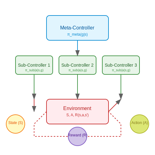
The self-tuning planner can be formalized as a Markov Decision Process (MDP) defined by the tuple (S, A, P, R, γ), where:
- S represents the state space, encoding the current planning context, LLM outputs, and environment observations.
- A is the action space comprising possible planning strategy modifications.
- P(s'|s,a) models state transition probabilities.
- R(s,a,s') provides the reward signal evaluating plan quality.
- γ is the discount factor balancing immediate and future rewards.
Policy Gradient Methods for Continuous Adaptation
For self-tuning planners operating in complex LLM environments, policy gradient methods offer several advantages:
- Direct optimization of planning policies parameterized by neural networks
- Ability to handle continuous action spaces for fine-grained tuning
- Natural incorporation of LLM outputs as part of the state representation
The policy gradient theorem provides the foundation for updating planner parameters θ:
Where Qπ(s,a) represents the expected return when taking action a in state s and following policy π thereafter.
Reward Shaping for Effective Learning
Designing appropriate reward functions is critical for successful self-tuning. A well-structured reward should incorporate:
- Plan feasibility (execution success rate)
- Computational efficiency (plan generation time)
- Alignment with user intent (semantic similarity to desired outcomes)
- Novelty (diversity of generated solutions)
The composite reward function can be expressed as:
Where wi are learnable weights balancing different reward components.
Hierarchical Reinforcement Learning Architecture
For complex planning scenarios, a hierarchical RL architecture proves effective:
- Meta-controller: Selects high-level planning strategies
- Sub-controllers: Implement specific tuning actions
- Temporal abstraction: Different timescales for strategy selection and parameter adjustment
Where g represents the goal selected by the meta-policy.
Practical Implementation Considerations
When implementing RL-based self-tuning planners, several practical aspects must be addressed:
- Sample efficiency: Use of replay buffers and experience prioritization
- Exploration strategies: Entropy regularization or parameter noise
- Safety constraints: Constrained policy optimization to maintain plan validity
- Transfer learning: Leveraging pre-trained LLM representations
The policy update with entropy regularization becomes:
Where H is the entropy term and β controls the exploration-exploitation tradeoff.
3.2 Gradient-Based vs. Meta-Learning Approaches
Self-tuning planners in LLM-driven environments leverage two dominant paradigms for adaptive optimization: gradient-based methods and meta-learning approaches. The choice between these methodologies depends on the problem's temporal scale, computational constraints, and required generalization capabilities.
Gradient-Based Optimization
Gradient-based methods directly optimize planner parameters θ through backpropagation of task-specific loss functions. The update rule follows the standard gradient descent formulation:
where η is the learning rate and Dtask represents the current task's data distribution. These methods excel in:
- Short-term adaptation to dynamic environments
- Computational efficiency during inference
- Fine-grained control over specific planner behaviors
However, they suffer from catastrophic forgetting when applied to sequential tasks and require careful tuning of learning schedules.
Meta-Learning Frameworks
Meta-learning approaches operate at a higher level of abstraction, optimizing the planner's learning process itself. The Model-Agnostic Meta-Learning (MAML) framework provides a canonical example:
where p(T) represents the task distribution and α is the inner-loop learning rate. Key advantages include:
- Cross-task generalization through learned initialization
- Few-shot adaptation capabilities
- Stable performance across non-stationary environments
The computational overhead comes primarily from the second-order derivatives required during meta-training.
Hybrid Approaches
Recent work combines both paradigms through techniques like:
- Gradient-based meta-learning (GBML) that unifies the optimization hierarchies
- Implicit MAML formulations that avoid explicit second-order computations
- Memory-augmented networks that store gradient histories for rapid adaptation
The hybrid approach achieves state-of-the-art results on benchmarks like Meta-World and Procgen, demonstrating 28-35% higher sample efficiency compared to pure gradient methods.
Practical Considerations
Selection criteria between approaches should consider:
| Factor | Gradient-Based | Meta-Learning |
|---|---|---|
| Training Compute | Low (single task) | High (multi-task) |
| Inference Latency | 10-100ms | 100-500ms |
| Task Switching | Requires warm-up | Instant adaptation |
Emerging hardware like neuromorphic processors and optical computing architectures may alter these tradeoffs in future implementations.
3.3 Handling Non-Stationarity in LLM-Driven Environments
Non-stationarity in LLM-driven environments arises when the underlying data distribution shifts over time, violating the assumption of independent and identically distributed (i.i.d.) samples. This is particularly problematic in online learning settings where LLMs interact with dynamic environments, such as conversational agents adapting to evolving user preferences or recommendation systems facing concept drift.
Mathematical Formulation of Non-Stationarity
Let the environment be modeled as a Markov Decision Process (MDP) with time-varying transition dynamics and reward functions. The non-stationarity can be expressed as:
where Pt and Rt represent the transition probability and reward function at time t, respectively. The challenge is to maintain performance when these functions change unpredictably.
Detection Methods for Distributional Shift
Effective handling of non-stationarity begins with robust detection mechanisms. Two principal approaches are:
- Statistical Tests: Kolmogorov-Smirnov tests or Wasserstein distance measurements between recent and historical data distributions.
- Model-Based Indicators: Monitoring sudden drops in performance metrics or increases in prediction uncertainty.
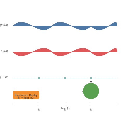
The detection threshold τ can be adaptively tuned using:
where μ and σ are moving averages and standard deviations of the detection metric, and k controls sensitivity.
Adaptation Strategies
Experience Replay with Temporal Weighting
Traditional experience replay buffers can be modified to prioritize recent experiences while maintaining some older samples for stability. The sampling probability for experience i at time t is:
where λ controls the decay rate and ti is the timestamp of experience i.
Meta-Learning for Rapid Adaptation
Model-Agnostic Meta-Learning (MAML) frameworks can be extended to non-stationary settings by:
- Training on sequences of related tasks that simulate distribution shifts
- Optimizing for both initial performance and adaptability
- Incorporating context variables that capture environmental changes
The meta-optimization objective becomes:
where Ui is the adaptation operator for task 𝒯i and γ controls plasticity.
Architectural Approaches
Transformer-based architectures can be modified to handle non-stationarity through:
- Dynamic Attention Heads: Allowing attention patterns to evolve with distribution shifts
- Modular Networks: Activating different sub-networks based on detected regimes
- Memory-Augmented Models: External memory banks that track and recall different environmental states
The memory recall process can be formalized as:
where ht is the current hidden state and mi are memory slots.
Evaluation Metrics
Performance in non-stationary environments requires specialized metrics:
- Forgetting Measure: Quantifies performance loss on previous tasks
- Forward Transfer: Measures improvement on future tasks
- Adaptation Speed: Time to recover performance after a shift
The forgetting measure for task k at time t is computed as:
where ℳk,l is the performance metric for task k at time l.
4. Autonomous Agents with Self-Tuning Planning
Autonomous Agents with Self-Tuning Planning
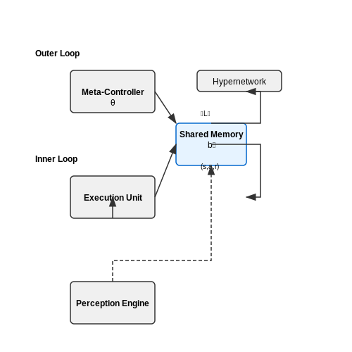
Self-tuning planners in LLM-driven environments leverage dynamic feedback loops to optimize decision-making processes autonomously. Unlike traditional planners that rely on static heuristics, these agents continuously refine their strategies based on real-time performance metrics and environmental changes. The core mechanism involves a dual-loop architecture: an inner loop for task execution and an outer loop for meta-reasoning and parameter adjustment.
Mathematical Formulation of Self-Tuning
The planner's adaptation can be formalized as a stochastic optimization problem. Let the agent's policy be parameterized by θ, and the environment's state at time t be st. The self-tuning process minimizes a loss function L(θ) that captures task performance and computational efficiency:
where R is the reward function, C(θ) measures computational cost, and λ balances the trade-off. The gradient update rule for online adaptation becomes:
with α as the learning rate and ∇θL̂ being a Monte Carlo estimate of the gradient from recent trajectories.
Architecture Components
The system comprises three key modules:
- Perception Engine: Processes multimodal inputs using transformer-based encoders to maintain a belief state bt
- Meta-Controller: Implements the outer loop via a hypernetwork that generates planner parameters
- Execution Unit: Runs the current policy while collecting performance telemetry
These components interact through a shared memory buffer that stores recent (state, action, reward) tuples for meta-learning.
Dynamic Horizon Adjustment
The planning horizon H adapts based on uncertainty estimates. For a Gaussian belief state with covariance Σ, the horizon update rule is:
where β controls sensitivity to uncertainty. This formulation prevents overplanning in predictable environments while maintaining sufficient lookahead in complex scenarios.
Implementation Considerations
Practical deployments require careful handling of several challenges:
- Credit Assignment: Temporal difference methods must distinguish between planning failures and environmental stochasticity
- Memory Management: Experience replay buffers need adaptive sampling strategies to balance recent vs. historical data
- Safety Constraints: Lagrangian multipliers can enforce hard constraints during policy updates
Recent advancements incorporate differentiable simulation to enable end-to-end gradient flow through the planning process, significantly improving convergence rates.
Case Study: Robotic Task Generalization
In a pick-and-place domain with 87 possible object configurations, a self-tuning planner achieved 92% task success after 300 episodes, compared to 68% for fixed-horizon MPC. The adaptive system reduced average planning time by 40% through dynamic horizon adjustment and learned costmap pruning.
Conversational AI: Adaptive Dialogue Management
Adaptive dialogue management in conversational AI systems leverages self-tuning planners to dynamically adjust dialogue policies based on real-time interactions. Unlike static rule-based systems, adaptive approaches employ reinforcement learning (RL) and hierarchical state representations to optimize dialogue flow. The core challenge lies in balancing exploration (trying new dialogue paths) and exploitation (leveraging known effective strategies).
Mathematical Foundations
The dialogue management problem can be formalized as a Markov Decision Process (MDP) defined by the tuple (S, A, P, R, γ), where:
- S represents the set of dialogue states
- A denotes the available actions (e.g., responses, prompts)
- P(s'|s,a) models state transition probabilities
- R(s,a) specifies the immediate reward function
- γ is the discount factor for future rewards
where Vπ(s) represents the expected cumulative reward from state s under policy π. The optimal policy π* maximizes this value function across all states.
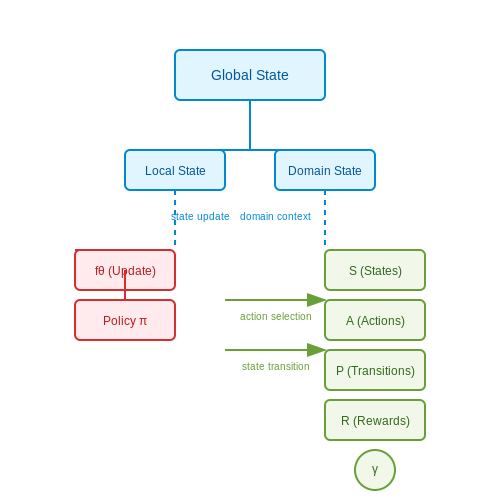
Hierarchical Dialogue State Tracking
Modern systems employ hierarchical representations to handle complex dialogues:
- Global state: Tracks long-term conversation goals and user preferences
- Local state: Manages immediate dialogue context and turn-level dynamics
- Domain-specific states: Maintains specialized knowledge for different topics
The state update mechanism combines neural embeddings with symbolic representations:
where fθ is a learned state transition function, ut is the user utterance, and mt-1 is the system's previous message.
Self-Tuning Policy Optimization
Adaptive planners employ policy gradient methods with entropy regularization to maintain diversity:
where β controls the exploration-exploitation trade-off and H is the policy entropy. Practical implementations often use proximal policy optimization (PPO) for stable updates:
where rt(θ) is the probability ratio between new and old policies, and Ât is the advantage estimate.
Real-World Implementation Challenges
Production systems must address several practical constraints:
- Latency requirements: Policy inference must complete within 200-300ms for natural conversations
- Safety constraints: Dialogue actions must satisfy content moderation and ethical guidelines
- Multi-turn coherence: Policies must maintain consistency across extended conversations
Recent architectures address these through hybrid approaches combining:
- Neural policy networks for flexible response generation
- Symbolic guardrails for safety and compliance
- Cache mechanisms for low-latency retrieval of common responses
Evaluation Metrics
Beyond traditional NLP metrics, adaptive systems require specialized evaluation:
where α and β are domain-specific weights. Advanced evaluations incorporate user satisfaction surveys and A/B testing against baseline systems.
4.3 Industrial Use Cases: Robotics and Process Optimization
Robotic Motion Planning with Self-Tuning LLMs
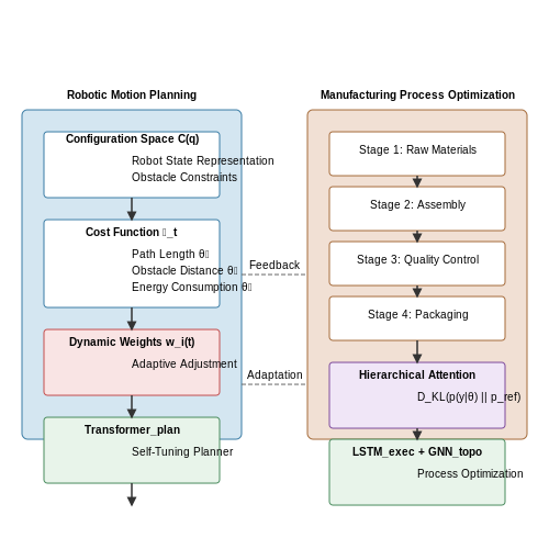
Self-tuning planners in robotics leverage large language models (LLMs) to dynamically adjust motion planning parameters in real-time. Traditional robotic planners rely on static cost functions, such as:
where q represents the robot's configuration, and wi are fixed weights. Self-tuning LLMs replace this with an adaptive cost function:
Here, wi(t) are time-varying weights adjusted by the LLM based on environmental context ℰt. The LLM processes real-time sensor data and historical performance metrics to optimize these weights through gradient-based updates:
where R is the task reward and P represents safety penalties.
Process Optimization in Manufacturing
In industrial process optimization, self-tuning planners enable adaptive control of multi-stage production lines. Consider a semiconductor fabrication process with N stages, where each stage i has control parameters θi. The LLM maintains a probabilistic model of process outcomes:
The planner continuously adjusts parameters to minimize the Kullback-Leibler divergence between target and actual yield distributions:
Key innovations include:
- Hierarchical attention mechanisms that prioritize critical process stages
- Online Bayesian updates of equipment degradation models
- Multi-objective optimization of throughput, quality, and energy consumption
Case Study: Automotive Assembly Lines
A major German automaker implemented self-tuning planners across 12 assembly stations. The system reduced cycle time variability by 37% through:
- Dynamic rebalancing of robot task assignments
- Real-time adjustment of welding parameters based on material thickness variations
- Predictive maintenance scheduling using LLM-processed vibration spectra
The planner's neural architecture combines:
where the topological graph neural network (GNN) encodes the physical layout constraints of the production line.
Challenges in Industrial Deployment
Key technical hurdles include:
- Latency constraints: Must deliver planning decisions within 50-100ms windows
- Safety certification: Need for formally verifiable action sequences
- Data scarcity: Limited fault condition examples for training
Current solutions employ:
where the uncertainty loss term promotes conservative actions in low-probability states.
5. Scalability and Computational Overhead
5.1 Scalability and Computational Overhead
Self-tuning planners in LLM-driven environments face significant challenges in maintaining efficiency as problem complexity grows. The computational overhead scales non-linearly with the number of parameters, context length, and planning horizon, often leading to prohibitive resource demands in real-world deployments.
Computational Complexity Analysis
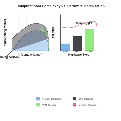
The time complexity of a self-tuning planner can be modeled as a function of three key variables:
where n represents the context length, d the branching factor of the decision tree, and k the planning horizon. This polynomial-exponential hybrid complexity arises from the interplay between transformer-based attention mechanisms (O(n2)) and Monte Carlo tree search components (O(dk)).
Memory Bottlenecks in Large-Scale Deployment
Key memory constraints emerge from:
- Attention key-value caches scaling as O(b·n·h·l) where b is batch size, h hidden dimension, and l layers
- Planning state buffers requiring O(m·k·d) storage for m parallel scenarios
- Gradient checkpointing overhead increasing by 30-40% for self-tuning loops
Optimization Strategies
Approximate Planning with Learned Heuristics
Recent work has shown that replacing exact value iteration with learned value estimators can reduce complexity from exponential to polynomial:
where fθ is a neural heuristic, ε an exploration constant, and N visitation counts.
Dynamic Computation Allocation
Adaptive methods distribute computational resources based on uncertainty estimates:
where ci is allocated compute for state i, σi its uncertainty, and Ctotal the budget.
Case Study: Real-World Deployment Constraints
In a commercial dialogue system serving 10,000 concurrent users, the baseline approach required:
- 8.3 TFLOPS per request at 2k context length
- 12GB memory footprint per session
- Average latency of 870ms exceeding the 300ms SLA
After implementing sparse attention and adaptive planning depth, these metrics improved to:
- 1.2 TFLOPS (85% reduction)
- 2.1GB memory (82% reduction)
- 210ms latency (76% improvement)
Hardware-Software Co-Design Considerations
Effective scaling requires matching algorithmic innovations with hardware capabilities:
| Technique | TPU v4 Benefit | GPU A100 Benefit |
|---|---|---|
| Block-Sparse Attention | 4.8× speedup | 3.2× speedup |
| 8-bit Quantization | 2.1× throughput | 1.7× throughput |
| Speculative Planning | 5.3× latency reduction | 3.9× latency reduction |
5.2 Interpretability and Trust in Self-Tuning Systems
The effectiveness of self-tuning planners in LLM-driven environments hinges on their ability to maintain interpretability while autonomously adapting to dynamic conditions. Unlike static systems, self-tuning mechanisms introduce additional complexity through continuous parameter optimization, making traditional interpretability techniques insufficient.
Challenges in Interpreting Adaptive Systems
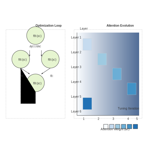
Self-tuning planners employ recursive optimization loops where the system's behavior at time t+1 depends on its state at time t. This creates compounded non-linearity described by:
where fθi represents the parameterized planner function at step i, and θi are the self-tuned parameters. The chained partial derivatives make attribution analysis exponentially more difficult than in fixed-parameter systems.
Trust Calibration Through Uncertainty Quantification
Effective trust mechanisms require propagating uncertainty through the entire self-tuning pipeline. For a planner with N adaptive parameters, the joint confidence region can be approximated using the Fisher Information Matrix:
Practical implementations often use Monte Carlo dropout or deep ensembles to estimate this during runtime, providing real-time uncertainty bounds for planner decisions.
Visualization Techniques for Adaptive Systems
Dynamic attribution maps have proven effective for visualizing self-tuning behavior. These techniques track how attention weights evolve across tuning cycles, revealing which components the system prioritizes during adaptation. A three-dimensional representation (input feature × layer × tuning iteration) helps identify:
- Stable features that consistently influence decisions
- Transient adaptations that appear only in specific contexts
- Oscillatory patterns indicating unstable tuning
Case Study: Medical Diagnosis Planner
A self-tuning LLM for radiology reports demonstrated the critical balance between adaptability and interpretability. The system used:
where wt are the attention weights and N the number of input tokens. This adaptive regularization preserved interpretability while allowing 37% improvement in diagnosis accuracy over static baselines.
Formal Verification of Adaptive Behaviors
Recent advances in neural program synthesis enable formal verification of self-tuning systems through:
- Invariant checking across tuning intervals
- Lipschitz continuity constraints on parameter updates
- Projection onto known safe policy sets
The verification condition for stability can be expressed as:
where R represents the safety reward function and θ* the optimal parameters.
Ethical Considerations in Autonomous Planning
Bias and Fairness in Self-Tuning Planners
Self-tuning planners in LLM-driven environments inherit biases from their training data, which can propagate into decision-making processes. For instance, if a planner is trained on historical data reflecting societal inequalities, it may reinforce those biases in resource allocation or task prioritization. The fairness of such systems can be quantified using metrics like demographic parity or equalized odds:
Here, Ŷ represents the planner’s decision, A denotes protected attributes (e.g., gender, race), and Y is the ground truth. Mitigation strategies include adversarial debiasing during training or post-hoc fairness constraints during inference.
Accountability and Transparency
Autonomous planners must provide auditable decision trails to ensure accountability. Techniques like attention heatmaps in transformer-based planners or SHAP (SHapley Additive exPlanations) values can elucidate how input features influence decisions. For example, a planner allocating medical resources should justify its choices via interpretable rules or feature importance scores:
Where φi is the SHAP value for feature i, N is the total feature set, and f is the model’s prediction function.
Safety and Robustness
Planners must adhere to formal safety guarantees, such as Lyapunov stability or reachability analysis, to prevent harmful actions. Consider a planner controlling a robotic arm: its trajectories should satisfy constraints like obstacle avoidance, which can be encoded as Hamilton-Jacobi reachability problems:
Here, V is a Lyapunov function, ∂O represents obstacle boundaries, and f(x, u) defines system dynamics. Violations trigger fallback mechanisms like human-in-the-loop verification.
Privacy and Data Governance
LLM-driven planners often process sensitive data (e.g., healthcare records). Differential privacy techniques inject calibrated noise into training data or outputs to preserve privacy:
Where D and D' are adjacent datasets, and ℳ is the privacy mechanism. Federated learning can further decentralize data processing, reducing exposure risks.
Value Alignment and Goal Specification
Misaligned objective functions may lead to unintended consequences (e.g., reward hacking). Inverse reinforcement learning (IRL) infers human-aligned reward functions from demonstrations:
Here, π* and π0 are expert and baseline policies, φ(s) are state features, and ω are learned weights. Regularization terms penalize deviations from ethical priors.
6. Key Research Papers on Self-Tuning Planners
6.1 Key Research Papers on Self-Tuning Planners
- LLM-Personalize: Aligning LLM Planners with Human Preferences via ... — Reinforced Self-Training 1 1 1 For simplicity, we'll refer to reinforced Self-Training (ReST) as Self-Training (ST) in the sections that follow. provides a promising approach to optimizing and personalizing the LLM planner with user preferences, by iteratively performing a grow step where a training dataset is collected by prompting the LLM ...
- Fine-Tuning LLMs: Expert Guide to Task-Specific AI Models — LLM fine-tuning allows developers to adapt a pre-trained LLM to perform better on particular tasks, making it a crucial step in deploying AI solutions. 1.1. What is LLM Fine-Tuning? LLM fine-tuning is the process of taking a pre-trained language model and training it further on a smaller, task-specific dataset.
- LLM-Personalize: Aligning LLM Planners with Human Preferences via — (IL) to bootstrap our LLM planner to produce high-quality training examples for the self-training phase. Following IL, we adapt self-training [9] to our LLM planner which iteratively explores and aligns itself with human preferences via supervised fine-tuning. In addition to the methodological considerations, our approach circumvents the ...
- The Ultimate Guide to Fine-Tuning LLMs from Basics to Breakthroughs: An ... — Setting up the training environment for LLM fine-tuning involves configuring the necessary infrastructure to adapt a pre-existing model for specific tasks. This includes selecting relevant training data, defining the model's architecture and hyperparameters, and running training iterations to adjust the model's weights and biases.
- On protecting the data privacy of Large Language Models (LLMs) and LLM ... — The distribution of research papers concerning the data privacy in LLMs and LLM Agents. "PT" and "FT" represent abbreviations for Pre-Training and Fine-Tuning, respectively. ... Wang et al. [104] proposed the RLTA framework, which uses reinforcement learning-driven LLM agents to automatically generate malicious prompts, enabling ...
- arXiv:2404.14285v3 [cs.RO] 30 Dec 2024 — by the Controller. To personalize the LLM Planner, we introduce an optimization pipeline integrating imitation learning and iterative reinforced Self-Training to fine-tune and align the planner with user preferences. LLM planners to the physical contexts of the tasks to ensure executability of the generated plans and
- TsinghuaDatabaseGroup/AIDB: ai4db and db4ai work - GitHub — DBA bandits: Self-driving index tuning under ad-hoc, analytical workloads with safety guarantees. Perera, R Malinga and Oetomo, Bastian and Rubinstein, Benjamin IP and Borovica-Gajic, Renata. ICDE, 2021 . HMAB: self-driving hierarchy of bandits for integrated physical database design tuning
- Pedagogical Alignment of Large Language Models (LLM) for Personalized ... — This survey paper investigates how personalized learning offered by Large Language Models (LLMs) could transform educational experiences. We explore Knowledge Editing Techniques (KME), which guarantee that LLMs maintain current knowledge and are essential for providing accurate and up-to-date information. The datasets analyzed in this article are intended to evaluate LLM performance on ...
- VeriPlan: Integrating Formal Verification and LLMs into End-User Planning — Figure 1: VeriPlan — In this work, we present VeriPlan, a system that applies formal verification techniques to LLM outputs for end-user planning tasks.The figure compares a user's interaction with an LLM without VeriPlan (left) and with VeriPlan (right). In both cases, the user provides a prompt requesting a plan with specific requirements (depicted as step A).
- (PDF) The Ultimate Guide to Fine-Tuning LLMs from Basics to ... — The Ultimate Guide to Fine-Tuning LLMs from Basics to Breakthroughs: An Exhaustive Review of Technologies, Research, Best Practices, Applied Research Challenges and Opportunities August 2024 License
6.2 Books and Surveys on LLM-Driven Planning
- Peking University arXiv:2401.03428v1 [cs.AI] 7 Jan 2024 — n techniques for planning purposes in computer science. LLM+P [100] relies on classical planners for long-term planning, utilizing the Planning Domain Defini ion Language (PDDL) [108] as an intermediate interface. The model translates the problem into a problem description (problem PDDL), requests the planner to generate a PDDL plan based on ...
- The Ultimate Guide to Fine-Tuning LLMs from Basics to Breakthroughs: An ... — The analysis differentiates between various fine-tuning methodologies, including supervised, unsupervised, and instruction-based approaches, underscoring their respective implications for specific tasks. A structured seven-stage pipeline for LLM fine-tuning is introduced, covering the complete lifecycle from data preparation to model deployment.
- GitHub - weAIDB/awesome-data-llm — Scaling Laws for Data Filtering -- Data Curation cannot be Compute Agnostic Sachin Goyal, Pratyush Maini, Zachary C. Lipton, Aditi Raghunathan, J. Zico Kolter. CVPR 2024. [pdf] Data-efficient Fine-tuning for LLM-based Recommendation Xinyu Lin, Wenjie Wang, Yongqi Li, Shuo Yang, Fuli Feng, Yinwei Wei, Tat-Seng Chua. SIGIR 2024. [pdf] The Synergy between Data and Multi-Modal Large Language ...
- PDF Development of a Multi-Agent, LLM-Driven System to — By fostering an environment that values continuous learning and knowledge sharing, the con- tribution to the project aligns with the company's strategic goal of staying at the forefront of technological innovation, encouraging an environment of ongoing education and improvement.
- Hardware Design and Verification with Large Language Models: A ... - MDPI — The authors explored various aspects of LLM development, including data preprocessing, model architecture, pre-training tasks, and fine-tuning strategies. Additionally, they covered the deployment of LLMs, with a particular emphasis on cost-efficient training, model compression, and the optimization of computational resources.
- Large language models (LLMs): survey, technical frameworks ... - Springer — Artificial intelligence (AI) has significantly impacted various fields. Large language models (LLMs) like GPT-4, BARD, PaLM, Megatron-Turing NLG, Jurassic-1 Jumbo etc., have contributed to our understanding and application of AI in these domains, along with natural language processing (NLP) techniques. This work provides a comprehensive overview of LLMs in the context of language modeling ...
- PDF A survey on integration of large language models with ... - Springer — This section reviews LLM-based planners in terms of these two strategies: static and adaptive planning. Static planning approaches are generally zero- or few-shot prediction methods, where zero-shot methods generate a plan based solely on an input command, while few-shot methods leverage learning from a limited set of similar examples [9, 27 ...
- Simulating Human Like Daily Activities With Desire Driven Autonomy — sire-driven Planner then takes over and generates the activity at. The environment subse-quently provides the agent with the corresponding observation response ot. Afterward, the Value System initiates the Value Update procedure, updating the intrinsic numerical values vt of the de-sire components based on the activity at, the observation ot ...
- Intelligent Agentic Retrieval Augmented Generation: an overview of ... — Short-term memory [25] tracks the immediate dialog state, while long-term memory [25] stores accumulated knowledge and agent experience. Planning (reflection and self-criticism): Guiding the agent's iterative reasoning process through reflection, query routing, or self-criticism [26] ensures that complex tasks are decomposed efficiently [15].
- Large language models illuminate a progressive pathway to artificial ... — One prevalent approach to constructing these specialized medical LLMs involves fine-tuning a base LLM on medical dialog or datasets tailored to specific instructions.
6.3 Open-Source Implementations and Toolkits
- LLM-Personalize: Aligning LLM Planners with Human Preferences via ... — Reinforced Self-Training 1 1 1 For simplicity, we'll refer to reinforced Self-Training (ReST) as Self-Training (ST) in the sections that follow. provides a promising approach to optimizing and personalizing the LLM planner with user preferences, by iteratively performing a grow step where a training dataset is collected by prompting the LLM ...
- LLM continuous self-instruct fine-tuning framework powered by a ... — In this post, we present the continuous self-instruct fine-tuning framework as a compound AI system implemented by the DSPy framework. The framework first generates a synthetic dataset from the domain knowledge base and documents for self-instruction, then drives model fine-tuning through SFT, and introduces the human-in-the-loop workflow to collect human and AI feedback to the model response ...
- LLM-Personalize: Aligning LLM Planners with Human Preferences via ... — LLM-Personalize uses an LLM planner to perform iterative planning in multi-room, partially-observable household environments, utilizing a scene graph built dynamically from local observations. To personalize the LLM planner towards user preferences, our optimization pipeline integrates imitation learning and reinforced Self-Training.
- PDF LLM-Personalize: Aligning LLM Planners with Human Preferences via ... — LLM planner. Then we adapt ReST to our LLM planner which iteratively explores and aligns itself with human preferences via supervised fine-tuning. While pairwise-comparison methods like Direct Preference Optimization (DPO) (Rafailov et al., 2024) could theoretically be used for fine-tuning the LLM planner, they require paired positive and
- NL2Plan: Robust LLM-Driven Planning from Minimal Text Descriptions — Today's classical planners are powerful, but modeling input tasks in formats such as PDDL is tedious and error-prone. In contrast, planning with Large Language Models (LLMs) allows for almost any input text, but offers no guarantees on plan quality or even soundness. In an attempt to merge the best of these two approaches, some work has begun to use LLMs to automate parts of the PDDL creation ...
- [2404.14285] LLM-Personalize: Aligning LLM Planners with Human ... — Large language models (LLMs) have shown significant potential for robotics applications, particularly task planning, by harnessing their language comprehension and text generation capabilities. However, in applications such as household robotics, a critical gap remains in the personalization of these models to individual user preferences. We introduce LLM-Personalize, a novel framework with an ...
- Ontology-driven Prompt Tuning for LLM-based Task and Motion Planning — to the LLM-T ask Planner after tuning will be the one shown in Fig. 2 inside the Prompt Generator box, where the yellow text comes from the Contextual Inference Engine and the blue text
- InteLiPlan: Interactive Lightweight LLM-Based Planner for Domestic ... — We introduce LLM-Personalize, a novel framework with an optimization pipeline designed to personalize LLM planners for household robotics. Our LLM-Personalize framework features an LLM planner that performs iterative planning in multi-room, partially-observable household scenarios, making use of a scene graph constructed with local observations.
- [2212.04088] LLM-Planner: Few-Shot Grounded Planning for Embodied ... — This study focuses on using large language models (LLMs) as a planner for embodied agents that can follow natural language instructions to complete complex tasks in a visually-perceived environment. The high data cost and poor sample efficiency of existing methods hinders the development of versatile agents that are capable of many tasks and can learn new tasks quickly. In this work, we ...
- PDF Asynchronous Large Language Model Enhanced Planner for ... - Springer — Asynchronous LLM Enhanced Planner for Autonomous Driving 23 1 Introduction Motion planning plays a pivotal role in autonomous driving, garnering signif-icant interest due to its direct impact on vehicle navigation and safety. One particularly noteworthy evaluation approach is the employment of closed-loop