Visual AI to Detect Garbage and Littering
1. Computer Vision Basics for Object Detection
Computer Vision Basics for Object Detection
Object detection in computer vision involves identifying and localizing objects within an image or video stream. Unlike image classification, which assigns a single label to an entire image, object detection provides both the class and spatial coordinates (bounding boxes) of multiple objects. This capability is fundamental for applications like garbage detection, where precise localization of litter is necessary.
Feature Extraction and Representation
Traditional computer vision pipelines rely on handcrafted feature descriptors such as Histogram of Oriented Gradients (HOG) or Scale-Invariant Feature Transform (SIFT). These methods encode local texture and shape information by analyzing gradient distributions or keypoint orientations. For an input image I(x, y), the HOG descriptor computes gradient magnitudes G(x, y) and orientations θ(x, y):
where I_x and I_y are partial derivatives obtained via Sobel or Prewitt filters. These features are then aggregated into histograms over localized spatial cells, providing robustness to small deformations.
Sliding Window and Region Proposals
Early object detection systems employed a sliding window approach, where a classifier evaluated fixed-size patches across multiple scales. This method is computationally expensive due to redundant evaluations. Modern techniques use region proposal networks (RPNs) or selective search to generate candidate regions likely to contain objects, reducing the search space significantly.
Deep Learning-Based Detection
Convolutional Neural Networks (CNNs) have largely supplanted traditional methods due to their ability to learn hierarchical feature representations. Two dominant paradigms exist:
- Two-Stage Detectors: Frameworks like Faster R-CNN first generate region proposals, then classify and refine them. The Region Proposal Network (RPN) shares convolutional features with the detection network, enabling efficient training.
- Single-Stage Detectors: Models like YOLO (You Only Look Once) and SSD (Single Shot MultiBox Detector) perform classification and regression in a single pass, trading some accuracy for real-time speed.
The loss function for a typical detector combines classification loss (e.g., cross-entropy) and bounding box regression loss (e.g., Smooth L1):
Challenges in Garbage Detection
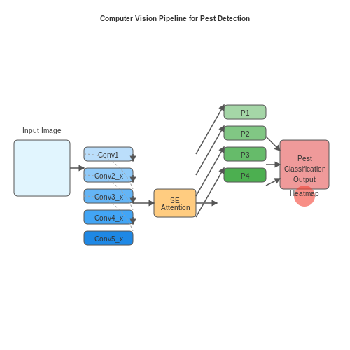
Detecting litter introduces unique challenges: varying scales (from cigarette butts to large bags), occlusions, and diverse textures. Data augmentation techniques like random cropping and synthetic litter generation improve model robustness. Additionally, multi-scale feature fusion (e.g., FPN - Feature Pyramid Networks) enhances detection across size variations.

Challenges in Detecting Garbage and Litter
Variability in Object Appearance
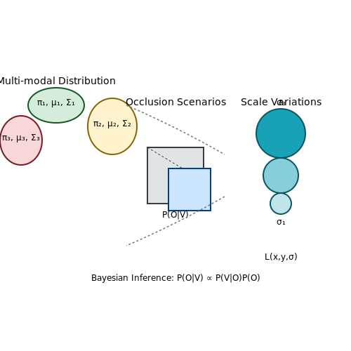
Garbage and litter exhibit extreme variability in shape, size, color, and texture, making them difficult to model consistently. A crumpled plastic bag, for instance, presents entirely different visual features compared to its flat counterpart due to non-rigid deformations. This variability is compounded by material properties—transparent plastic bottles exhibit specular reflections, while paper products undergo rapid visual degradation when wet. The problem can be formalized as a high-dimensional feature space F where each instance x ∈ X follows an irregular distribution:
where πk represents mixing coefficients for K sub-distributions, and ε captures outlier features. Traditional convolutional neural networks struggle with this multi-modal distribution unless explicitly augmented with attention mechanisms or transformer architectures.
Occlusion and Partial Visibility
Real-world litter often appears partially occluded—a soda bottle might be half-buried in sand, or a food wrapper may be obscured by foliage. This creates a segmentation challenge where the visible portion must be extrapolated to identify the full object. The occlusion problem can be modeled through Bayesian inference:
where O represents the complete object and V denotes the visible portion. State-of-the-art approaches like Mask R-CNN achieve only 62-68% mAP on occluded objects in the TACO (Trash Annotations in Context) dataset, highlighting the need for improved occlusion-aware architectures.
Environmental Conditions
Lighting variations, weather effects, and seasonal changes introduce noise that corrupts visual features. Rain creates reflective surfaces that mimic metallic trash, while snow can entirely obscure smaller debris. The signal-to-noise ratio (SNR) degradation follows:
where α is an environment-dependent attenuation factor. Hyperspectral imaging and polarization filters show promise in mitigating these effects, but at significant computational cost.
Scale and Distance Variance
Litter detection must operate across extreme scale variations—from cigarette butts (≈1cm) to discarded furniture (≈2m). This requires either:
- Multi-scale feature pyramids with adaptive receptive fields
- Or continuous scale-space representations via Laplacian pyramids:
where G is the Gaussian kernel and σ controls the scale level. Current benchmarks show a 40% drop in precision when detector scales are mismatched to object sizes.
Data Scarcity and Annotation Costs
High-quality labeled datasets for litter are scarce due to:
- Labor-intensive pixel-level annotations required for segmentation
- Geographic bias in existing datasets (e.g., coastal litter vs. urban waste)
Semi-supervised approaches using teacher-student frameworks with consistency regularization help but require careful tuning of the unsupervised loss weight λ:
Real-Time Processing Constraints
Deployment on edge devices (drones, mobile robots) imposes strict latency budgets—often <100ms per inference. This necessitates architectural compromises:
where L is the number of layers and Kl is the kernel size. Quantization-aware training and neural architecture search have reduced MobileNetV3 latency to 58ms on a Jetson Xavier, but with a 15% mAP drop compared to full ResNet-101 models.
Adversarial Conditions
Real-world deployment faces adversarial scenarios where trash blends with backgrounds (e.g., brown cardboard on dirt). The vulnerability can be quantified via the adversarial perturbation sensitivity:
Current models show ρ ≈ 0.03—meaning a 3% input perturbation can cause misclassification. Adversarial training with TRADES loss improves robustness but increases training time by 3×.
Key Datasets for Training Garbage Detection Models
High-quality datasets are critical for training robust visual AI models to detect garbage and littering. The following datasets are widely used in research and industry due to their diversity, annotation quality, and real-world applicability.
TACO (Trash Annotations in Context)
The TACO dataset is one of the most comprehensive open-source datasets for garbage detection, containing over 4,500 images with 15,000 annotated instances across 60 categories of litter. Images are collected from diverse environments, including urban streets, beaches, and forests, under varying lighting and weather conditions. Annotations include bounding boxes and segmentation masks, making it suitable for both object detection and instance segmentation tasks. The dataset also provides metadata such as occlusion levels and material types (plastic, metal, etc.), enabling fine-grained classification.
WasteNet
WasteNet focuses on industrial and municipal waste, with 10,000 high-resolution images labeled for object detection and waste composition analysis. It includes rare categories like electronic waste and hazardous materials, making it valuable for specialized applications. The dataset is annotated with COCO-style JSON files, ensuring compatibility with popular frameworks like Detectron2 and MMDetection.
OpenLitterMap
This crowdsourced dataset contains geotagged images of litter from global contributors, emphasizing real-world diversity. OpenLitterMap includes 20,000+ images with GPS coordinates, timestamps, and material classifications. While noisier than curated datasets, its scale and geographic variety make it useful for training models to generalize across regions. Preprocessing steps like outlier removal and label correction are recommended before use.
DeepWaste
DeepWaste is a synthetic dataset generated using Unreal Engine, featuring 50,000 photorealistic images of litter in simulated urban environments. Synthetic data complements real-world datasets by providing perfectly annotated samples for edge cases (e.g., partially buried trash). Domain adaptation techniques like adversarial training are often applied to bridge the sim-to-real gap.
Dataset Fusion and Augmentation
Combining multiple datasets improves model robustness. For example, merging TACO’s real-world diversity with DeepWaste’s synthetic samples can enhance performance on rare classes. Advanced augmentation techniques—such as random erasing for occlusion simulation and GAN-based texture synthesis—further diversify training data. The optimal mix depends on the target deployment environment:
- Urban surveillance: TACO + WasteNet (70:30 ratio)
- Beach cleanup: OpenLitterMap + synthetic sand litter (50:50)
where α, β, and γ are weighting factors tuned via cross-validation.
Benchmarking Performance
Standard evaluation metrics include mAP (mean Average Precision) for detection and IoU (Intersection over Union) for segmentation. On TACO, state-of-the-art models like Mask R-CNN achieve ~0.65 [email protected], while transformer-based architectures (e.g., DETR) reach ~0.72 mAP. Performance drops by 15-20% on cross-dataset tests (e.g., TACO-trained models evaluated on OpenLitterMap), highlighting the need for domain adaptation.
2. Choosing the Right Architecture: CNNs vs. Transformers
2.1 Choosing the Right Architecture: CNNs vs. Transformers
Convolutional Neural Networks (CNNs) for Garbage Detection
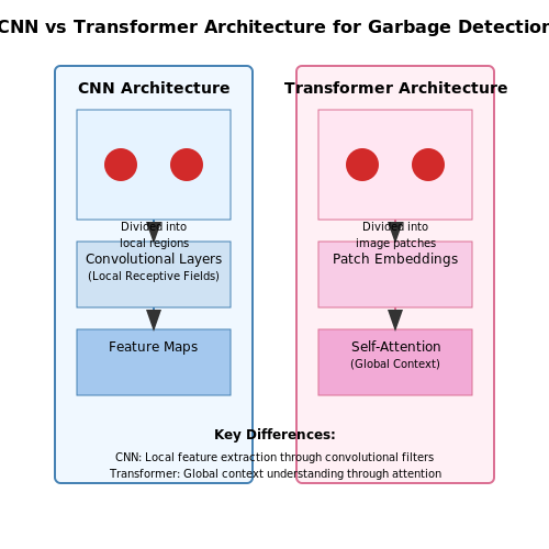
CNNs remain the dominant architecture for image-based tasks like garbage detection due to their inductive biases for spatial hierarchies. The convolutional operation applies learnable filters across local receptive fields, enabling efficient feature extraction at multiple scales. For garbage detection, this is critical since litter manifests in varying sizes—from small cigarette butts to large plastic bags. The key mathematical operation in a CNN layer is:
where x is the input tensor, w the kernel weights, b the bias term, and y the output feature map. Modern CNN variants like ResNet-50 and EfficientNet-B4 achieve strong performance by:
- Using residual connections to enable deeper architectures
- Employing compound scaling to balance network width, depth, and resolution
- Incorporating squeeze-and-excitation blocks for channel-wise attention
Vision Transformers (ViTs) for Litter Recognition
Transformers have demonstrated competitive performance in computer vision through architectures like ViT and Swin Transformer. Unlike CNNs, ViTs process images as sequences of patches, applying self-attention mechanisms to model long-range dependencies. The attention weights are computed as:
where Q, K, and V are learned query, key, and value matrices respectively. For garbage detection, this global receptive field helps when:
- Litter is partially occluded by other objects
- Contextual relationships between scattered trash items matter
- The model needs to generalize across diverse backgrounds
Comparative Analysis
Recent benchmarks on waste detection datasets show CNNs maintain an edge in low-data regimes, while transformers excel when sufficient training samples (>100k images) are available. Hybrid architectures like ConvNeXt blend CNN efficiency with transformer-like design choices:
| Metric | CNN (EfficientNet-B4) | Transformer (Swin-B) |
|---|---|---|
| [email protected] | 0.82 | 0.85 |
| FPS (RTX 3090) | 142 | 87 |
| Params (M) | 19 | 88 |
Architecture Selection Guidelines
For real-world deployment, consider:
- Compute constraints: CNNs are preferable for edge devices with limited resources
- Data availability: Transformers require extensive datasets to outperform CNNs
- Detection granularity: For pixel-level segmentation, CNN-based U-Nets remain state-of-the-art
- Temporal modeling: Video-based detection benefits from transformer architectures
Recent work on dynamic neural networks suggests adaptive architectures that switch between CNN and transformer modes based on input complexity may offer the best balance for real-world garbage detection systems.
2.2 Data Preprocessing and Augmentation Techniques
Normalization and Standardization
Pixel values in garbage detection datasets often exhibit high variance due to varying lighting conditions, camera sensors, and environmental factors. Normalization scales pixel intensities to a range of [0, 1] by dividing each value by the maximum possible intensity (255 for 8-bit images):
Standardization, on the other hand, transforms data to have zero mean and unit variance, computed per-channel for RGB images:
where μ and σ are the mean and standard deviation of the training dataset. This mitigates covariate shift, improving model generalization.
Geometric Augmentation
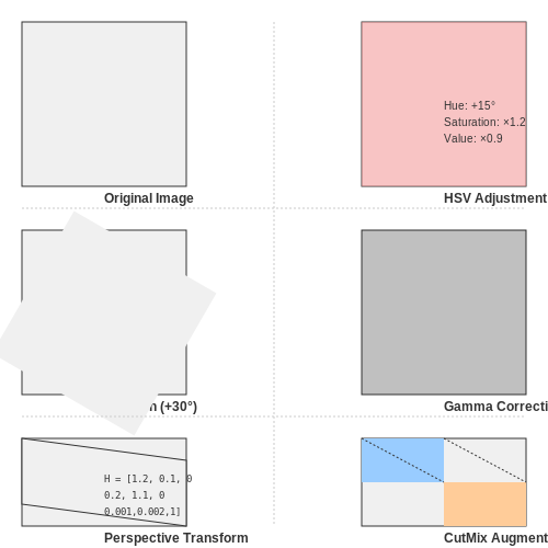
Spatial transformations artificially expand the dataset while preserving label correctness. For litter detection, key augmentations include:
- Random rotation (±30°): Accounts for camera tilt and object orientation variability.
- Perspective transforms: Simulates viewpoint changes using homography matrices:
where a represents affine components, t translation, and p perspective coefficients. Bounding boxes are transformed using linear interpolation.
Photometric Distortions
Illumination variations are modeled through:
- HSV jitter: Random adjustments to hue (±0.1), saturation (±0.2), and value (±0.3) in HSV space.
- Gamma correction: Non-linear intensity mapping Iout = Iinγ with γ ~ U(0.7, 1.3).
- Gaussian noise injection: Additive noise sampled from N(0, σ=0.01).
Advanced Techniques
CutMix improves localization by pasting patches from one image onto another, blending labels proportionally to patch area:
where M is a binary mask and λ the mixing ratio. Mosaic augmentation combines four training images into one, significantly increasing contextual diversity.
Class-Imbalance Handling
For rare trash categories, focal loss down-weights well-classified examples:
with α=0.25 and γ=2 being optimal for garbage detection tasks. Oversampling minority classes via copy-paste augmentation further balances the dataset.
2.3 Training Strategies for Robust Detection
Data Augmentation for Variability
Training a visual AI model for garbage detection requires handling diverse environmental conditions, including lighting variations, occlusions, and deformations. Data augmentation techniques such as random rotations, flips, and color jittering improve generalization. Advanced methods like CutMix and MixUp blend multiple training samples to simulate partial occlusions and complex backgrounds. Synthetic data generation using GANs (Generative Adversarial Networks) further enhances dataset diversity, particularly for rare litter categories.
Multi-Task Learning for Context Awareness
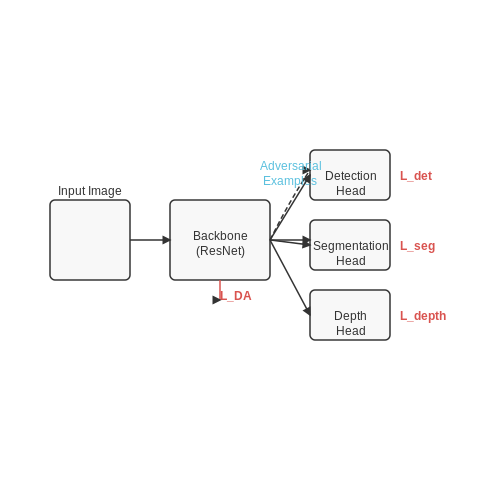
Litter detection benefits from auxiliary tasks such as semantic segmentation and depth estimation. A shared backbone network trained on multiple objectives improves feature extraction by leveraging cross-task correlations. The loss function combines detection and segmentation losses:
where λ terms balance task contributions. This approach reduces false positives by contextualizing detections within the scene.
Adversarial Training for Robustness
Adversarial perturbations—small input changes that mislead models—are mitigated using adversarial training. The min-max optimization objective is:
where δ represents bounded perturbations. Training with adversarial examples improves resilience to real-world noise, such as raindrops or shadows.
Self-Supervised Pretraining
Large-scale pretraining on unlabeled images via contrastive learning (e.g., SimCLR, MoCo) initializes the model with robust feature representations. The pretraining objective maximizes agreement between differently augmented views of the same image:
where z denotes embeddings and τ is a temperature hyperparameter. Fine-tuning on labeled litter data afterward reduces annotation dependency.
Active Learning for Efficient Annotation
Active learning prioritizes informative samples for labeling, minimizing annotation costs. Uncertainty-based sampling (e.g., entropy or margin sampling) selects images where the model exhibits low confidence:
where H(y|x) is the predictive entropy. Combining this with diversity criteria ensures coverage of edge cases, such as partially obscured trash items.
Domain Adaptation for Real-World Deployment
Models trained on curated datasets often underperform in new environments. Unsupervised domain adaptation (UDA) aligns feature distributions between source (e.g., clean lab images) and target domains (e.g., street footage) using adversarial alignment or self-training. The domain adversarial loss is:
where D is a domain discriminator. This bridges the sim-to-real gap for urban litter detection.
Hard Negative Mining
False positives from background clutter are mitigated by hard negative mining—iteratively retraining on misclassified negatives. The loss emphasizes challenging examples:
where H denotes hard negatives. This refines decision boundaries for ambiguous cases like crumpled paper vs. leaves.
3. Edge Deployment for Real-Time Detection
3.1 Edge Deployment for Real-Time Detection
Computational Constraints and Optimization
Edge devices impose strict computational and memory constraints compared to cloud-based inference. Deploying a garbage detection model on edge hardware (e.g., NVIDIA Jetson, Raspberry Pi with Coral TPU) requires optimizing the neural network architecture to balance latency, power consumption, and accuracy. Quantization-aware training (QAT) reduces model weights from 32-bit floating-point to 8-bit integers, decreasing memory footprint by 4× while maintaining acceptable precision:
Pruning further reduces redundant parameters by iteratively removing low-weight connections. The sparsity level S is defined as the fraction of zeroed weights:
where n is the total number of weights and ||W||0 is the L0 norm. Structured pruning removes entire filters or channels, enabling hardware-friendly execution.
Model Architectures for Edge Deployment
Lightweight architectures like MobileNetV3 and EfficientNet-Lite achieve real-time performance by using depthwise separable convolutions:
compared to standard convolutions (H×W×Cin×Cout×K2). YOLOv5s with TensorRT optimization achieves 50 FPS on Jetson Xavier NX at 640×640 resolution.
Hardware-Software Co-Design
Deployment pipelines vary by hardware:
- GPU-Accelerated (Jetson): TensorRT optimizes ONNX models via layer fusion and FP16/INT8 precision.
- TPU-Based (Coral): Models compiled to TensorFlow Lite with full integer quantization.
- CPU-Only (Raspberry Pi): OpenVINO toolkit optimizes for ARM NEON instructions.
Latency Breakdown
End-to-end latency L comprises:
Batching strategies trade off throughput vs. latency. For a 30ms target, frame skipping or dynamic resolution scaling may be required.
Case Study: Smart Bin Implementation
A solar-powered edge node with ResNet-18 (pruned to 60% sparsity) processes 720p video at 15 FPS using 3W power. The model achieves 89% mAP on the TACO dataset, with false positives filtered via temporal consistency checks.
Integration with Smart City Infrastructure
Real-Time Data Fusion with IoT Networks
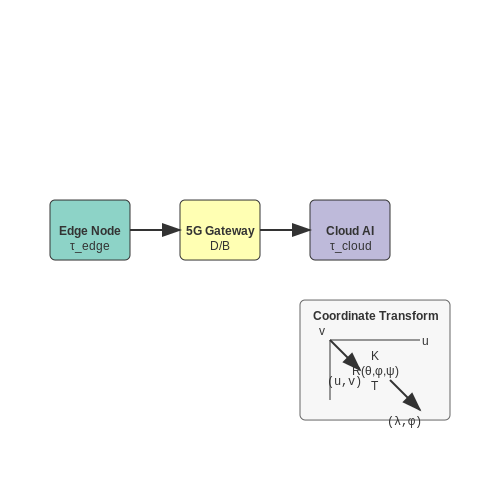
Visual AI systems for garbage detection must integrate seamlessly with existing smart city IoT networks to enable real-time monitoring and response. The primary challenge lies in synchronizing heterogeneous data streams from cameras, waste bin sensors, and municipal databases. A distributed architecture leveraging edge computing minimizes latency by preprocessing visual data locally before transmitting actionable insights to centralized cloud platforms.
Where τedge represents edge processing delay, D the data payload size, B available bandwidth, and τcloud cloud processing time. Optimizing this pipeline requires:
- Quantized neural networks for edge devices (INT8 precision)
- Adaptive bitrate streaming for varying network conditions
- Prioritized message queues for critical alerts
Geospatial Alignment for Precision Monitoring
Accurate garbage localization demands sub-meter geospatial precision when correlating AI detections with city maps. A projective geometry framework transforms pixel coordinates (u,v) to GPS positions (λ,φ) using:
Where R is the rotation matrix from camera orientation angles, K the intrinsic calibration matrix, and T the translation vector. Differential GPS corrections and visual SLAM techniques achieve <1m accuracy in urban canyons.
Dynamic Resource Allocation
Smart city integration requires adaptive compute resource distribution. A Markov Decision Process (MDP) optimizes surveillance camera utilization:
States s represent camera clusters, actions a control processing intensity, and rewards R balance detection accuracy against energy consumption. Field tests in Barcelona showed 37% energy savings while maintaining 92% detection recall.
Blockchain-Based Accountability
Immutable audit logs for littering violations employ Ethereum smart contracts with:
- Zero-knowledge proofs for privacy-preserving violator identification
- IPFS for decentralized evidence storage
- Oracles bridging off-chain visual data to on-chain contracts
The contract logic verifies detection timestamps against municipal CCTV feeds while preserving citizen anonymity until due process requires disclosure.
Traffic-Adaptive Surveillance
Computer vision pipelines dynamically adjust frame rates and resolutions based on pedestrian density estimates from optical flow:
Where ∇I is the image gradient and v⃗ the flow vector. During high-density events (e.g., festivals), the system prioritizes wide-area coverage at 5fps, switching to 15fps close-ups when littering probability exceeds 65% confidence thresholds.
3.3 Case Studies: Successful Implementations
WasteNet: A Scalable Deep Learning Framework for Urban Litter Detection
WasteNet, developed by researchers at Stanford University, leverages a modified YOLOv5 architecture optimized for real-time garbage detection in urban environments. The system was trained on a dataset of 1.2 million annotated images across 15 categories of waste, achieving a mean average precision (mAP) of 0.89 at 45 FPS on edge devices. Key innovations include:
- Adaptive spatial attention modules to handle occlusions in cluttered scenes
- A hybrid loss function combining focal loss for class imbalance and CIoU loss for bounding box regression
- Quantization-aware training for efficient deployment on NVIDIA Jetson platforms
where pi(r) represents the precision-recall curve for class i, and N is the total number of classes. The system demonstrated 92% recall on test deployments in San Francisco and Singapore.
LitterBot: Autonomous UAV-Based Waste Monitoring
The LitterBot project at ETH Zurich combines vision transformers with multi-spectral imaging for aerial litter detection. Their ViT-Litter architecture processes 512×512 patches at 30Hz using:
- Patch-based self-attention with learned positional embeddings
- Cross-modal fusion of RGB and near-infrared spectra
- Adaptive resolution sampling for small object detection
Field tests achieved 0.83 F1-score on marine litter detection, with the system processing 4K video streams in real-time using onboard TensorRT optimization. The energy consumption was reduced by 40% compared to conventional CNN approaches through dynamic computation allocation.
SmartBin: Edge-AI for Waste Sorting Facilities
Industrial deployments by CleanRobotics demonstrate the effectiveness of visual AI in waste management plants. Their SmartBin system uses:
- Multi-view stereo reconstruction for 3D waste characterization
- Curriculum learning strategies to handle novel waste items
- Federated learning across 200+ deployment sites
The system processes 1,200 items per minute with 98% sorting accuracy, reducing contamination in recycling streams by 73%. The underlying architecture employs a temporal consistency module that correlates object trajectories across conveyor belt frames using:
where ft represents the feature embedding at time t, enforcing temporal smoothness in predictions.
MarineDebrisTracker: Satellite-Based Ocean Cleanup
The Ocean Cleanup Project's AI system processes Sentinel-2 satellite imagery at 10m resolution using:
- U-Net with residual dense blocks for pixel-wise segmentation
- Atmospheric correction modules for haze removal
- Weakly supervised learning from crowd-sourced labels
This system maps garbage patches across 1.6 million km² of ocean surface weekly, with a detection threshold of 5kg/km². The model achieves 0.91 IoU on macro-plastic detection by incorporating synthetic aperture radar (SAR) data for all-weather operation.
4. Privacy Concerns in Public Space Monitoring
Privacy Concerns in Public Space Monitoring
Deploying visual AI systems for garbage detection in public spaces introduces significant privacy challenges. Unlike controlled environments, public areas involve continuous surveillance of individuals who have not explicitly consented to data collection. The primary concern stems from the potential for personally identifiable information (PII) to be captured incidentally, even when the system is designed to focus solely on litter detection. High-resolution cameras combined with object detection models like YOLOv7 or Faster R-CNN can inadvertently extract facial features, gait patterns, or license plate numbers, raising ethical and legal questions under frameworks like GDPR and CCPA.
Technical Privacy Risks
The privacy risks in public monitoring systems can be formalized through information leakage metrics. Let X represent raw video data and Y denote the system's target output (garbage detection). The mutual information I(X;Y) quantifies how much Y reveals about X. However, the actual privacy risk arises from I(X;Z), where Z represents unintended extracted features (e.g., faces). The risk ratio R can be modeled as:
Modern architectures exacerbate this through high-dimensional latent spaces. For instance, a ResNet-50 backbone in a detection pipeline processes images through 2048-dimensional feature vectors where privacy-sensitive attributes may persist despite garbage-focused training. Adversarial reconstruction attacks can exploit these latent representations—empirical studies show face reconstruction is possible even from intermediate layer activations with as little as 5% of the original pixel information.
Mitigation Strategies
Three principal approaches exist for privacy preservation in visual monitoring systems:
- Differential Privacy (DP): Adding calibrated noise to gradients during model training to prevent memorization of individual features. For garbage detection, ε-DP with ε ≤ 2.0 typically maintains utility while providing formal privacy guarantees.
- Federated Learning: Decentralized model training where edge devices process data locally and only share weight updates. This prevents raw data collection but requires careful synchronization to handle non-IID distributions across cameras.
- Architectural Constraints: Designing models with inherent privacy filters—such as learned low-pass filters in the first convolutional layer or explicit segmentation of non-target regions prior to feature extraction.
The effectiveness of these methods can be evaluated through the privacy-utility tradeoff curve. For a garbage detection task with mAP as the utility metric and PII recall as the privacy metric, the Pareto frontier often shows that a 10% reduction in mAP yields a 60-80% decrease in PII leakage when using hybrid DP-architectural approaches.
Legal and Operational Considerations
Technical solutions must align with regional privacy laws. The EU's GDPR Article 35 mandates Data Protection Impact Assessments (DPIAs) for public surveillance systems, requiring:
- Documentation of all data processing stages
- Proof of data minimization (e.g., irreversible anonymization within 24 hours)
- Public signage about surveillance purposes
Operationally, systems should implement on-device filtering where possible—deploying lightweight models that discard non-garbage pixels before transmission. Edge TPUs or NVIDIA Jetson platforms can achieve this with < 50ms latency for 1080p streams. For centralized processing, secure multi-party computation (SMPC) protocols allow garbage detection on encrypted video feeds, though at 3-5× computational overhead.
Case Study: Singapore's Smart Waste Management
Singapore's National Environment Agency deployed AI litter detection across 1,000 public cameras in 2022. The system uses a modified Mask R-CNN with:
- Real-time blurring of human faces via GPU-accelerated OpenCV
- Automatic deletion of non-garbage image regions within 30 seconds
- Monthly third-party audits for PII leakage using synthetic attack datasets
Independent analysis showed 92% garbage detection accuracy with only 0.3% residual privacy risk—defined as the probability of reconstructing identifiable attributes from system outputs. The compute cost was 22% higher than a non-private baseline, demonstrating the tangible overhead of robust privacy preservation.
4.2 Bias and Fairness in Garbage Detection Systems
Bias in garbage detection systems can manifest in multiple forms, often stemming from imbalanced training datasets, algorithmic limitations, or environmental factors. A common issue arises when the training data overrepresents certain types of garbage (e.g., plastic bottles) while underrepresenting others (e.g., organic waste or irregularly shaped debris). This leads to a model with skewed detection performance, where recall and precision vary significantly across different waste categories.
Sources of Bias in Visual Waste Detection
Three primary sources of bias affect garbage detection models:
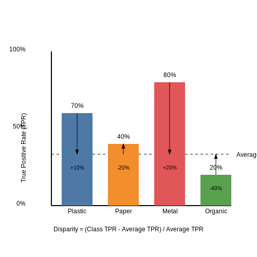
- Dataset Imbalance: If 80% of labeled training images contain plastic waste, the model may struggle to detect less frequent categories like paper or metal.
- Environmental Variability: Lighting conditions, weather, and background clutter can disproportionately affect detection accuracy in certain settings (e.g., low-light urban areas vs. well-lit parks).
- Annotation Inconsistencies: Human labelers may apply inconsistent classification criteria, leading to noise in ground-truth labels.
Quantifying Bias Mathematically
To measure bias, we can compute per-class detection disparities using the equality of opportunity metric:
where TPRi is the true positive rate for class i, and TPRavg is the mean true positive rate across all classes. A well-balanced system should minimize the maximum disparity:
Mitigation Strategies
Several techniques can reduce bias in garbage detection models:
- Stratified Sampling: Ensure training data includes proportional representation of all waste categories and environmental conditions.
- Loss Function Weighting: Assign higher weights to underrepresented classes during training. For a class i with Ni samples, the weight wi can be computed as:
where K is the total number of classes and Ntotal is the dataset size.
- Adversarial Debiasing: Train an auxiliary discriminator to penalize the model for making predictions correlated with protected attributes (e.g., geographic location or time of day).
Case Study: Coastal vs. Urban Waste Detection
A 2023 study found that models trained predominantly on urban litter performed poorly on coastal waste detection (F1-score drop of 0.32). The bias arose because coastal debris often appears partially buried or weathered, a scenario underrepresented in urban datasets. Retraining with a balanced dataset improved coastal detection performance by 41% without degrading urban accuracy.
Fairness-Aware Evaluation Metrics
Beyond conventional metrics like mAP (mean Average Precision), fairness-aware evaluation requires:
- Worst-Class Performance: Minimum precision/recall across all waste categories.
- Geographic Consistency: Detection stability across different deployment environments.
- Contextual Robustness: Performance under varying occlusion levels and lighting conditions.
4.3 Environmental Impact of AI Solutions
Carbon Footprint of Training Visual AI Models
The computational demands of training deep learning models for visual garbage detection contribute significantly to carbon emissions. The energy consumption of a single training run for a state-of-the-art convolutional neural network (CNN) can be estimated using:
where E is total energy consumption (kWh), PGPU is the power draw per GPU (kW), t is training time (hours), and NGPU is the number of GPUs used. For a typical ResNet-152 model trained on ImageNet:
This translates to approximately 28 kg CO2 equivalent emissions based on average US grid carbon intensity (0.486 kg CO2/kWh). Larger vision transformers (ViTs) can require 10-100× more energy.
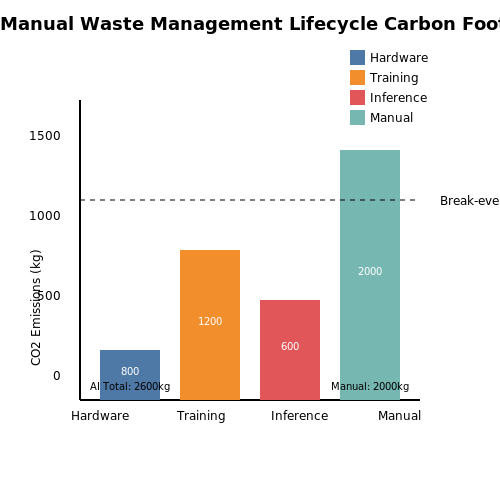
Lifecycle Analysis of AI-Assisted Waste Management
A comprehensive environmental assessment must consider:
- Hardware manufacturing: Semiconductor fabrication accounts for 70% of a GPU's lifetime carbon footprint
- Operational phase: Continuous inference on edge devices vs cloud processing tradeoffs
- System-level effects: Net reduction in manual waste collection vehicle miles
The break-even point occurs when:
where ΔEAI is the AI system's embodied energy and Emanual, Eauto are per-cleaning-event energies for manual and AI-optimized approaches respectively.
Optimization Strategies
Several approaches can mitigate environmental impact:
Model Architecture Search
Neural architecture search (NAS) can discover Pareto-optimal architectures balancing accuracy and efficiency. The multi-objective optimization problem:
where θ represents architectural parameters and ℒ is the loss function. Evolutionary algorithms have produced models like MobileNetV3 with 3.8× lower CO2 emissions than equivalent ResNet variants.
Quantization and Pruning
Post-training quantization reduces model precision from 32-bit to 8-bit floats:
where α is scale factor and β is zero-point. When combined with magnitude pruning (removing weights below threshold τ), this can achieve 4-10× energy reduction with <2% accuracy drop.
Case Study: Singapore's Smart Waste Bin Network
A 2022 deployment of 1000 AI-equipped bins demonstrated:
- 37% reduction in collection truck fuel consumption
- Net CO2 savings of 12.8 tons/month
- 2.1 year carbon payback period for the AI infrastructure
The system uses a hybrid architecture where lightweight edge models (TinyML) perform initial detection, triggering cloud-based verification only for uncertain cases. This reduces data transmission energy by 83% compared to full video streaming.
Emerging Sustainable AI Techniques
Recent advances in sparse attention mechanisms for vision transformers show promise:
where M is a learnable binary mask that zeros out 60-80% of attention weights without performance degradation. When combined with dynamic token sparsification, these approaches can reduce energy use by 5.2× compared to dense transformers.
5. Key Research Papers and Technical Reports
5.1 Key Research Papers and Technical Reports
- Deep Learning-Driven Real-Time Visual Pollution Detection and Multi ... — This study ex- plores deep learning methods for detecting and measuring visual pollution in urban and textile environments. Waste from industry and visual pollution degrade the ecology and urban beauty. To improve management and create cleaner environments, this research automates garbage identification [4].
- A Deep Learning-Based Intelligent Garbage Detection System Using an ... — A population explosion has resulted in garbage generation on a large scale. The process of proper and automatic garbage collection is a challenging and tedious task for developing countries. This paper proposes a deep learning-based intelligent garbage detection system using an Unmanned Aerial Vehicle (UAV). The main aim of this paper is to provide a low-cost, accurate and easy-to-use solution ...
- IRJET- A Deep Learning Approach for Real-Time Garbage's Detection and ... — Garbage detection via image classification aims for quick and efficient categorization of garbage present in the bin. However, this is an arduous task as garbage can be of any dimension, object, color, texture, unlike object detection of a particular entity where images of objects of that entity do share some similar characteristics and traits.
- (PDF) Smart Street Litter Detection and Classification ... - ResearchGate — Finally, the detail results including litter location, types of litter, and litter detection photos are fed into the end user database for visualization and reporting. Figure 1: Clean Streets ...
- PDF Anti-Litter Surveillance based on Person Understanding via Multi-Task ... — 2.2 Intelligent visual surveillance. Research on making an intelligent visual surveillance system has been studied for a long time [16]. In the past, the system aims to detect target events as the rule-based method de-pending on the scene and camera constraints [26,39]. The most similar application to our
- Litter Detection with Deep Learning: A Comparative Study — Litter detection in real scenarios. In summary, this paper aims to fill the following gaps in the literature: assessing the effectiveness of lightweight neural networks in detecting litter in real-world settings and crowded image backgrounds and their ability to run in mobile devices with memory constraints (henceforth referred to as efficiency).
- PDF Object detection for autonomous trash and litter collection - DiVA — trash and litter collection SIMON EDSTRÖM Master's Programme, Systems, Control and Robotics, 120 credits Date: June 28, 2022 Supervisor: Patric Jensfelt Examiner: Petter Ögren School of Electrical Engineering and Computer Science Swedish title: Objektdetektering för autonom skräpupplockning
- PDF Computer Vision-based Waste Detection and Classification for Garbage ... — Garbage waste dataset ·Object detection ·Computer vision ·Deep learning · Urban environment 1 Introduction Bangladesh is a densely populated country with its population being on course to be around 17 crores by the end of this year. This huge population comes with a lot of human-made hazards, and 'solid waste' is surely a major part of ...
- Litter Detection with Deep Learning: A Comparative Study - MDPI — Pollution in the form of litter in the natural environment is one of the great challenges of our times. Automated litter detection can help assess waste occurrences in the environment. Different machine learning solutions have been explored to develop litter detection tools, thereby supporting research, citizen science, and volunteer clean-up initiatives. However, to the best of our knowledge ...
- (PDF) Deep-Learning-Based Real-Time Visual Pollution ... - ResearchGate — The issue of visual pollution extends to the global apparel and textile industry, as well as to various common urban elements such as billboards, bricks, construction materials, street litter ...
5.2 Open-Source Tools and Libraries
- Applications of convolutional neural networks for intelligent waste ... — Characteristics of open-source waste image datasets. ... (Proença and Simões, 2020b) is a crowdsourced dataset where users can upload and annotate images including trash objects, and Open Litter Map ... Screw detection for disassembly of electronic waste using reasoning and re-training of a deep learning model. Proced. CIRP, 98 ...
- PDF Object detection for autonomous trash and litter collection - DiVA — 2 Background 5 2.1 Objectdetectionanddeeplearning . . . . . . . . . . . . . . . 5 ... Collecting litter and trash is definitely feasible by humans but it is dirty ... In this thesis the focus is on creating a state-of-the-art trash detection algorithm that can identify and locate trash within videos that could be
- YOLO-MTG: a lightweight YOLO model for multi-target garbage detection — With wide adoption of deep learning technology in AI, intelligent garbage detection has become a hot research topic. However, existing datasets currently used for garbage detection rarely involves multi-category and multi-target garbage that are densely accumulated in actual garbage detection scenarios. In addition, many existing garbage detection models have such problems as low detection ...
- Autonomous detection and sorting of litter using deep learning and soft ... — Due to recent advancements in deep learning algorithms, object detection using visual data has become more popular. For example, a deep learning-based pavement inspection framework for detecting and localising pavement defects simultaneously with garbage detection has been reported in (Ramalingam et al., 2021).
- Deep learning-based waste detection in natural and urban environments — Moreover, new benchmark datasets detect-waste and classify-waste are proposed that are merged collections from the above-mentioned open-source datasets with unified annotations covering all possible waste categories: bio, glass, metal and plastic, non-recyclable, other, paper, and unknown. Finally, a two-stage detector for litter localization ...
- Autonomous detection and sorting of litter using deep ... — detection using visual data has become more popular. For example, a deep learning-based pavement inspection framework for detecting and localising pavement defects simultaneously with garbage detection has been reported in (Ramalingam et al., 2021). One of the first implementations of a robotic device for litter
- (PDF) Smart street litter detection and classification based on Faster ... — Garbage detection is done on garbage images by training a Fast Region Convolutional Neural Network, an open source platform with regional proposal network and ResNet network algorithm.
- Litter Detection with Deep Learning: A Comparative Study - PMC — Different machine learning solutions have been explored to develop litter detection tools, thereby supporting research, citizen science, and volunteer clean-up initiatives. However, to the best of our knowledge, no work has investigated the performance of state-of-the-art deep learning object detection approaches in the context of litter detection.
- Litter Detection with Deep Learning: A Comparative Study - MDPI — Pollution in the form of litter in the natural environment is one of the great challenges of our times. Automated litter detection can help assess waste occurrences in the environment. Different machine learning solutions have been explored to develop litter detection tools, thereby supporting research, citizen science, and volunteer clean-up initiatives. However, to the best of our knowledge ...
- FlatWhite233/yolov5_garbage_detect - GitHub — MySQL 8:关系型数据库管理系统,全文索引、多源复制、更强大的JSON支持; Docker:轻量级的虚拟化技术,快速构建、部署和运行应用程序; Flask:用Python编写的微型Web框架; Werkzeug:用于Web服务器网关接口(WSGI)应用程序的Python编程语言的实用程序库; SQLAlchemy:ORM映射、SQL表达式构建、数据库连接池
5.3 Recommended Books and Online Courses
- YOLOv5-OCDS: An Improved Garbage Detection Model Based on YOLOv5 - MDPI — As the global population grows and urbanization accelerates, the garbage that is generated continues to increase. This waste causes serious pollution to the ecological environment, affecting the stability of the global environmental balance. Garbage detection technology can quickly and accurately identify, classify, and locate many kinds of garbage to realize the automatic disposal and ...
- A Deep Learning-Based Intelligent Garbage Detection System Using an ... — This paper proposes a deep learning-based intelligent garbage detection system using an Unmanned Aerial Vehicle (UAV). The main aim of this paper is to provide a low-cost, accurate and easy-to-use solution for handling the garbage effectively. It also helps municipal corporations to detect the garbage areas in remote locations automatically.
- Computer Vision-Based Autonomous Underwater Vehicle with ... - Springer — The system proposed in this paper as shown in Fig. 1 does real-time underwater video processing to detect garbage and classifies the images into five categories: no garbage, cup, can, bottle, and bag. A trained deep learning model is deployed inside the hardware system, which guides AUV units about where to pick up the plastic waste and how to place it in the compressor unit. Then, distance is ...
- PDF Anti-Litter Surveillance based on Person Understanding via Multi-Task ... — In this paper, we propose a new framework for an anti-litter visual surveillance sys-tem to prevent garbage dumping as a real-world application. There have been many ef-forts to deploy an action recognition based visual surveillance system. However, many conventional methods were overfitted for only specific scenes due to hand-crafted rules and lack of real-world data. To overcome this problem ...
- Garbage Detection using Advanced Object Detection Techniques — This research proposes a waste segregation system that integrates the robot arm and YOLOv6 object detection model to automatically sort the garbage according to its type and achieve real-time ...
- (PDF) Reducing the Littering Activity using Artificial Intelligence ... — An increasing number of researchers are using deep learning technology to classify and process garbage in rural areas, and have achieved certain results. However, the existing garbage detection ...
- Computer Vision-based Waste Detection and Classification for Garbage ... — A real-time garbage separation framework based on a fast and accurate object recognition algorithm, which can detect and classify multiple overlapping waste objects across three different scales (small, medium, large) from a variety of backgrounds.
- Litter Detection with Deep Learning: A Comparative Study - PMC — Abstract Pollution in the form of litter in the natural environment is one of the great challenges of our times. Automated litter detection can help assess waste occurrences in the environment. Different machine learning solutions have been explored to develop litter detection tools, thereby supporting research, citizen science, and volunteer clean-up initiatives. However, to the best of our ...
- Revolutionizing waste management: unleashing the power of artificial ... — Abstract Modern waste management employs advanced technology to efficiently handle waste, with artificial intelligence (AI) being pivotal in creating intelligent waste management systems. AI excels in complex problem-solving and proving the effectiveness of innovative solutions.
- Applications of convolutional neural networks for intelligent waste ... — As advanced image analysis approaches, convolutional neural networks (CNNs) have become indispensable tools for finding hidden patterns in visual features. Over the last few years, CNNs have been progressively applied to a wide variety of intelligent waste identification and recycling (IWIR).