Contrastive Captioning Models
1. Key Concepts and Definitions
1.1 Key Concepts and Definitions
Contrastive Learning Framework
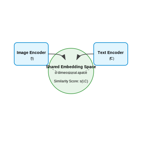
Contrastive captioning models operate within a contrastive learning framework, where the objective is to learn a joint embedding space that maximizes agreement between paired image-caption samples while minimizing agreement for unpaired samples. Given an image I and its corresponding caption C, the model learns a similarity function s(I, C) such that:
This is achieved through a dual-encoder architecture, where image and text inputs are processed by separate encoders fI and fC, producing normalized embeddings in a shared d-dimensional space. The similarity score is typically computed as the dot product of these embeddings:
InfoNCE Loss Function
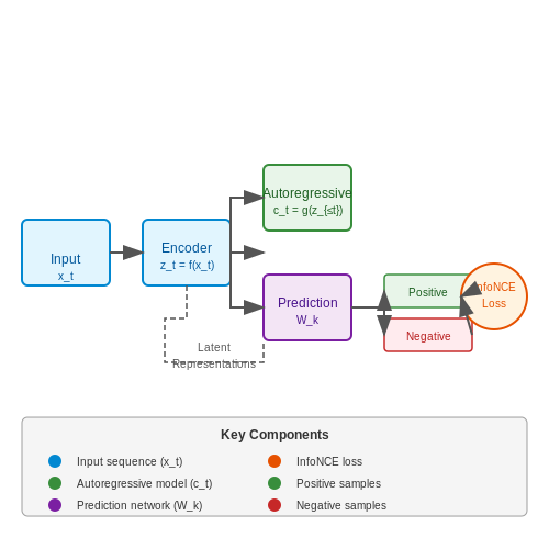
The training objective for contrastive captioning models is typically formulated using the InfoNCE (Noise Contrastive Estimation) loss, which originates from self-supervised learning literature. For a batch of N image-caption pairs, the loss for the i-th pair is:
where τ is a temperature parameter controlling the sharpness of the distribution. The total loss is symmetric with respect to images and captions, computed as:
Cross-Modal Attention Mechanisms
Advanced contrastive captioning models incorporate cross-modal attention to enable fine-grained alignment between visual regions and textual tokens. Given image features V ∈ ℝm×d and text features T ∈ ℝn×d, the cross-attention computes:
where Wq, Wk, Wv are learned projection matrices. This attention mechanism allows the model to establish region-word correspondences without explicit supervision.
Hard Negative Mining
Effective contrastive learning requires careful construction of negative samples. Hard negative mining strategies are critical for improving model discriminability:
- In-batch negatives: All non-matching pairs within a batch serve as negatives
- Memory bank negatives: Maintain a queue of embeddings from previous batches
- Adversarial negatives: Generate challenging negatives through gradient-based methods
The hardness of negatives is often controlled through temperature scaling in the loss function, with lower temperatures emphasizing harder negatives.
Pre-training and Fine-Tuning Paradigms
Modern contrastive captioning models follow a two-stage training process:
- Pre-training: Large-scale learning on noisy web-scale image-text pairs using contrastive objectives
- Fine-tuning: Task-specific adaptation using smaller, curated datasets with additional supervision
The pre-training stage typically employs massive datasets like LAION-5B or Conceptual Captions, while fine-tuning uses domain-specific data such as COCO or Flickr30k for downstream tasks.
Contrastive Learning in Vision-Language Models
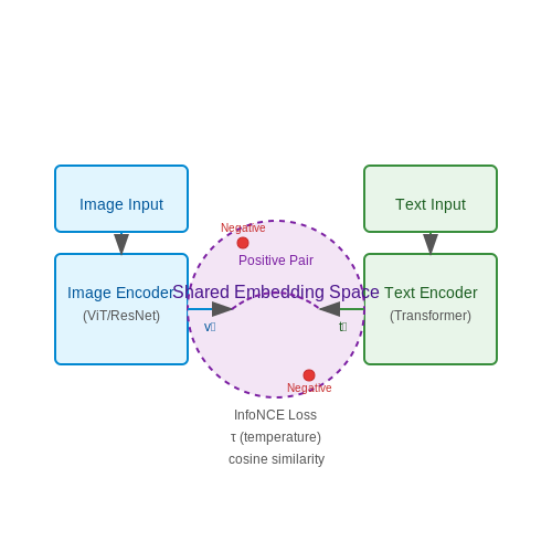
Contrastive learning forms the backbone of modern vision-language models by aligning representations of images and text in a shared embedding space. The core objective is to maximize similarity between positive pairs (correct image-text matches) while minimizing similarity for negative pairs (incorrect matches). This approach leverages the InfoNCE loss, a variant of noise-contrastive estimation, which operates on a batch of N image-text pairs:
Here, s(vi, ti) denotes the cosine similarity between the i-th image embedding vi and its corresponding text embedding ti, while τ is a temperature parameter controlling the sharpness of the distribution. The denominator sums over all possible negative pairs within the batch, creating a computationally efficient approximation of the full negative set.
Dual-Encoder Architecture
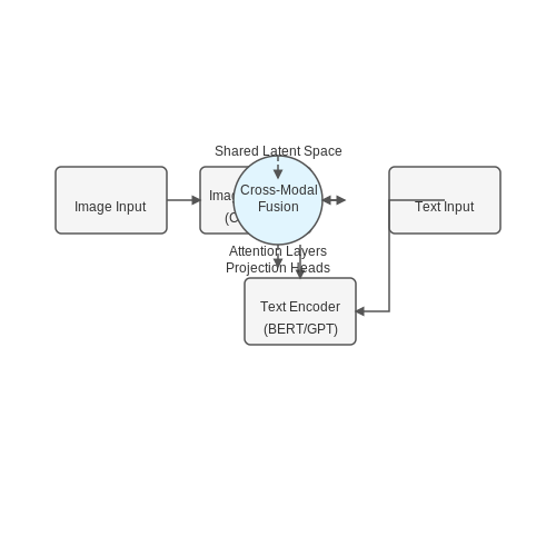
State-of-the-art implementations like CLIP and ALIGN employ a dual-encoder design:
- Image encoder: Typically a Vision Transformer (ViT) or ResNet, mapping images to a d-dimensional latent space
- Text encoder: Usually a transformer (e.g., BERT) processing tokenized text into the same d-dimensional space
The training dynamics create an emergent property where the dot product vTt approximates the log probability of the image-text pair being matched. This allows zero-shot classification by computing similarity between an image and class-descriptive prompts (e.g., "a photo of a {class}").
Hard Negative Mining
Advanced variants address the limitation of random in-batch negatives through:
Where 𝒩i contains semantically similar but incorrect pairs, identified via:
- Cross-modal retrieval (top-k similar but non-matching pairs)
- Intra-modal clustering (texts/images near the anchor in embedding space)
Modality Gap Analysis
The inherent discrepancy between visual and linguistic distributions manifests as a non-zero mean distance between image and text embeddings. Recent work quantifies this through:
Mitigation strategies include:
- Post-hoc projection networks (e.g., linear layers trained post-contrastive learning)
- Adversarial alignment during training
- Triplet losses with margin constraints
Scaling Laws and Batch Effects
Empirical studies reveal logarithmic improvements in downstream task performance with respect to batch size B:
Where α ≈ 0.1 and β is architecture-dependent. This relationship holds until B ≈ 105, beyond which gradient noise becomes dominant. Distributed training techniques like gradient sharding enable effective batch sizes up to 220 in production systems.
Role of Captioning in Multimodal Learning
Semantic Alignment Between Modalities
Captioning serves as a critical bridge between visual and textual modalities in multimodal systems. The process involves learning a joint embedding space where semantically similar concepts from different modalities are mapped close together. Given an image x and its corresponding caption y, contrastive models optimize an objective function that maximizes the mutual information between paired samples while pushing apart unpaired ones:
where f and g are modality-specific encoders, and τ is a temperature parameter controlling the sharpness of the distribution. This alignment enables zero-shot transfer capabilities, as demonstrated by CLIP's ability to classify images using text prompts without explicit training.
Attention Mechanisms in Cross-Modal Learning
Modern captioning models employ transformer-based architectures with cross-attention layers that dynamically compute relevance between visual regions and textual tokens. The attention weights αij between image region i and word j are computed as:
where Qj represents the query vector for the j-th textual token, Ki is the key vector for the i-th image region, and dk is the dimension of the key vectors. This mechanism allows the model to ground linguistic concepts in specific visual features, enabling fine-grained multimodal understanding.
Information Bottleneck Perspective
From an information theory viewpoint, captioning creates a compressed representation that preserves the most relevant information for downstream tasks. The optimal caption y for image x minimizes:
where t represents task-relevant variables, and β controls the trade-off between compression and preservation of predictive information. This formulation explains why automatically generated captions often omit visually salient but task-irrelevant details.
Evaluation Metrics and Their Limitations
Standard metrics like BLEU and CIDEr measure n-gram overlap with reference captions but fail to capture semantic adequacy. Emerging alternatives include:
- CLIPScore: Measures cosine similarity between image and caption embeddings in CLIP space
- UMIC: Computes the mutual information between image and text representations
- Visual Grounding Accuracy: Evaluates whether caption phrases correctly localize to image regions
Recent work shows these metrics correlate better with human judgment than traditional n-gram measures, with CLIPScore achieving 0.28 Spearman correlation with human ratings compared to 0.18 for BLEU-4 on the COCO dataset.
Applications in Multimodal Pretraining
Contrastive captioning forms the foundation for state-of-the-art multimodal architectures like:
- Flamingo: Uses gated cross-attention to interleave pretrained vision and language models
- CoCa: Jointly trains contrastive and generative objectives with a shared encoder
- BLIP-2: Bootstraps vision-language pretraining with frozen image encoders and large language models
These models demonstrate emergent capabilities in visual question answering, image-text retrieval, and multimodal reasoning, with BLIP-2 achieving 85.0% accuracy on VQAv2 without task-specific fine-tuning.
2. Encoder-Decoder Frameworks
Encoder-Decoder Frameworks
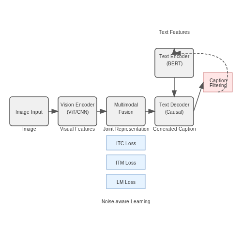
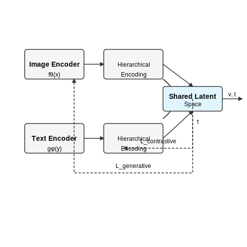
Encoder-decoder architectures form the backbone of modern contrastive captioning models, enabling the joint embedding of visual and textual data into a shared latent space. The encoder processes raw input data (images or text) into dense vector representations, while the decoder reconstructs or generates outputs conditioned on these embeddings. For vision-language tasks, this typically involves a dual-stream architecture where image and text encoders operate in parallel.
Mathematical Formulation
Given an image x and its corresponding caption y, the encoder functions fθ and gφ map these inputs to a d-dimensional embedding space:
The contrastive learning objective maximizes the similarity between matched image-text pairs while minimizing it for mismatched pairs. This is formalized using a temperature-scaled cosine similarity metric:
where τ is a learned temperature parameter controlling the sharpness of the similarity distribution.
Architecture Variants
Modern implementations employ several key architectural innovations:
- Transformer-based encoders: Vision transformers (ViTs) process images as sequences of patches, while text encoders use token-level self-attention.
- Cross-modal attention: Late fusion layers enable inter-modal interaction through attention mechanisms before the final embedding.
- Hierarchical encoding: Multi-scale feature extraction preserves both local and global semantic information.
Training Dynamics
The training process involves two complementary loss terms:
where the contrastive term aligns embeddings across modalities, and the generative term (typically a cross-entropy loss) ensures the decoder can reconstruct captions from visual embeddings. The hyperparameter λ balances these objectives.
Implementation Considerations
Practical implementations must address several challenges:
- Batch construction: Large batch sizes are critical for effective contrastive learning, requiring memory-efficient implementations.
- Embedding normalization: L2 normalization of output embeddings stabilizes training and improves performance.
- Asymmetric architectures: Image and text encoders often use different depths and widths optimized for their respective modalities.
Recent advances like CLIP and ALIGN demonstrate that properly scaled encoder-decoder frameworks can achieve remarkable zero-shot transfer capabilities, with the image encoder effectively learning visual concepts that align with the semantic space of the text encoder.
2.2 Contrastive Loss Functions
Contrastive loss functions are fundamental to training contrastive captioning models, as they enforce similarity between paired embeddings while pushing apart unrelated pairs. The core idea is to minimize the distance between positive pairs (e.g., an image and its correct caption) while maximizing the distance for negative pairs (e.g., an image and a mismatched caption).
Mathematical Formulation
The contrastive loss function can be derived from the InfoNCE (Noise Contrastive Estimation) objective, which maximizes the mutual information between positive pairs. Given a batch of N image-caption pairs, the loss for a single positive pair (i, j) is:
where si,j is the cosine similarity between the image embedding vi and caption embedding tj, and τ is a temperature hyperparameter controlling the sharpness of the distribution.
Temperature Scaling
The temperature parameter τ plays a critical role in contrastive learning. A lower τ sharpens the similarity distribution, making the model more selective, while a higher τ smooths the distribution, allowing for softer discrimination. Optimal τ values are typically found empirically, often in the range [0.01, 0.1].
Hard Negative Mining
To improve model robustness, hard negative mining is often employed. Instead of sampling random negatives, the loss is computed using the most challenging negatives within a batch:
where Nh represents the set of hard negatives, typically chosen as the top-k most similar but incorrect pairs.
Symmetrized Loss
For bidirectional alignment, a symmetrized version of the loss is often used, combining both image-to-text and text-to-image objectives:
This ensures that the model learns a coherent joint embedding space from both directions.
Practical Considerations
- Batch Size: Larger batches provide more negative samples, improving the quality of the learned embeddings. However, memory constraints often limit batch sizes in practice.
- Normalization: Embeddings are typically L2-normalized to constrain the similarity scores to [-1, 1].
- Gradient Issues: The exponential terms in the loss can lead to numerical instability. Log-sum-exp tricks or gradient clipping are often used to mitigate this.
Pretraining and Fine-Tuning Strategies
Contrastive Pretraining Objectives
Contrastive captioning models leverage multimodal pretraining objectives that align visual and textual embeddings in a shared latent space. The core loss function is typically a variant of the InfoNCE objective, which maximizes the mutual information between matched image-text pairs while minimizing similarity for negative samples:
where v represents visual features, t denotes text embeddings, s(·,·) is a similarity function (often cosine similarity), and τ is a temperature parameter controlling the sharpness of the distribution. The negative samples t'∈N are typically mined in-batch or through hard negative mining strategies.
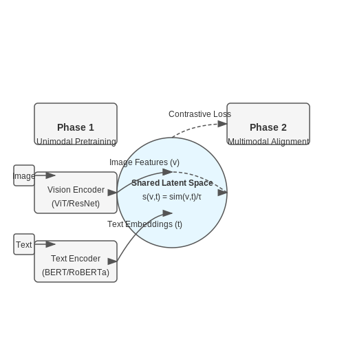
Two-Phase Training Protocol
State-of-the-art implementations employ a two-phase approach:
- Phase 1 - Unimodal Pretraining: Vision encoders (ViT, ResNet) are pretrained on large-scale image datasets (ImageNet-21k, JFT-300M) using supervised or self-supervised objectives (MAE, MoCo v3). Text encoders (BERT, RoBERTa) are pretrained on web-scale text corpora using masked language modeling.
- Phase 2 - Multimodal Alignment: The pretrained encoders are jointly optimized on image-text pairs (Conceptual Captions, LAION) using contrastive losses with adaptive gradient clipping (max norm typically 1.0-2.0) and learning rate warmup (5-10% of total steps).
Adaptive Fine-Tuning Techniques
For downstream tasks, several adaptation strategies prove effective:
where m is a binary mask implementing:
- Partial Fine-Tuning: Only the top k layers of each encoder are updated (typically 6-12 for transformer-based models)
- Adapter Layers: Small bottleneck MLPs inserted between transformer layers, freezing original parameters
- LoRA: Low-rank decomposition of weight updates ΔW = BA where rank(r) ≪ dmodel
Gradient Accumulation Strategies
For large batch contrastive learning with limited hardware, gradient accumulation with synchronized batch norms is critical. The effective batch size Beff becomes:
Typical configurations use Blocal=32-128 per GPU with Naccum=4-8 steps, achieving Beff in the range of 8k-32k. The learning rate should scale as η∝√Beff to maintain stability.
Temperature Parameter Scheduling
The contrastive loss temperature τ requires careful tuning. Recent work implements:
where t is the training progress (0→1), with typical values τmin=0.01, τmax=0.1, and λ=5. This annealing schedule prevents early overfitting to easy negatives while maintaining gradient stability.
3. Data Preparation and Augmentation
3.1 Data Preparation and Augmentation
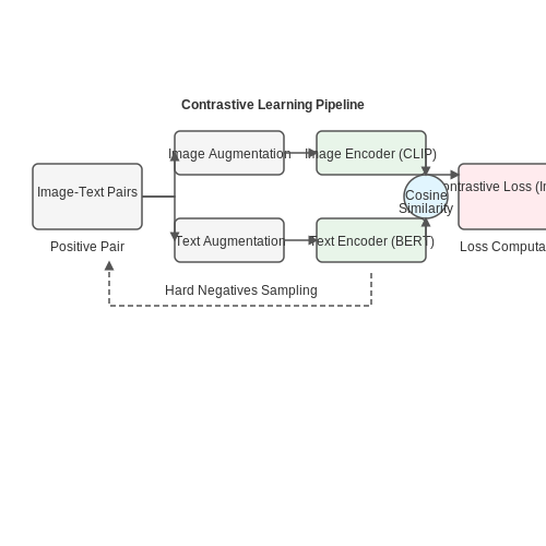
Contrastive captioning models rely on high-quality paired image-text datasets, where the alignment between visual and textual modalities must be explicitly optimized. The data preparation pipeline involves several critical steps: raw data collection, preprocessing, and augmentation. Each stage must be carefully designed to ensure the model learns robust cross-modal representations.
Raw Data Collection and Filtering
Large-scale datasets like Conceptual Captions or COCO provide image-text pairs, but noise and misalignments are common. Advanced filtering techniques include:
- Semantic similarity scoring: Compute embeddings for both images (using a pretrained vision encoder like CLIP) and text (using a language model like BERT), then filter pairs with low cosine similarity.
- Deduplication: Remove near-duplicate images using perceptual hashing or feature clustering.
- Language quality checks: Filter captions with low readability scores, excessive punctuation, or non-descriptive content.
Text Preprocessing and Tokenization
Textual data undergoes normalization, including lowercasing, punctuation stripping, and stopword removal (optional, depending on the model). Tokenization is typically performed using subword methods like Byte Pair Encoding (BPE) or WordPiece. For contrastive learning, the tokenized text is embedded into a fixed-length vector space:
where L is the sequence length and d is the embedding dimension. Positional embeddings are added to preserve order information.
Image Preprocessing and Feature Extraction
Images are resized to a fixed resolution (e.g., 224×224) and normalized using dataset statistics. Pretrained convolutional networks (e.g., ResNet, ViT) extract visual features:
where H, W, and C denote height, width, and channel dimensions. Global average pooling often reduces this to a 1D feature vector.
Augmentation Strategies for Contrastive Learning
Data augmentation is crucial for improving model robustness. For images, standard techniques include:
- Random cropping and resizing with area ratios between 0.8 and 1.0.
- Color jittering (brightness, contrast, saturation, hue adjustments).
- Gaussian blurring with kernel sizes sampled uniformly from [0.1, 2.0].
For text, augmentation is more challenging but can include:
- Synonym replacement using WordNet or contextual word embeddings.
- Back-translation (translate to an intermediate language and back).
- Random masking of non-essential words (e.g., adjectives, adverbs).
Negative Sampling for Contrastive Objectives
Contrastive models require negative samples—mismatched image-text pairs—to learn discriminative features. Two common strategies are:
- In-batch negatives: Use all non-matching pairs within a mini-batch.
- Hard negatives: Mine semantically similar but incorrect pairs using nearest-neighbor search in embedding space.
The contrastive loss (e.g., InfoNCE) is then computed as:
where τ is a temperature hyperparameter and sim denotes cosine similarity.
Dataset Splits and Evaluation Protocols
Standard splits (70% train, 15% validation, 15% test) are common, but cross-dataset evaluation (e.g., training on Conceptual Captions and testing on COCO) better assesses generalization. Metrics include:
- Recall@K: Percentage of queries where the correct match is in the top-K retrieved items.
- Median rank: Median position of the correct match in retrieved results.
3.2 Hyperparameter Tuning
Hyperparameter optimization in contrastive captioning models is critical for balancing the trade-off between alignment quality and computational efficiency. Unlike traditional captioning models, contrastive approaches involve dual-objective optimization—maximizing similarity between matched image-text pairs while minimizing it for mismatched pairs. The key hyperparameters include temperature scaling, batch size, learning rate scheduling, and projection head dimensions.
Temperature Scaling (τ)
The temperature parameter τ controls the sharpness of the softmax distribution in the contrastive loss function. A lower τ amplifies the differences between similarity scores, while a higher τ produces a smoother distribution. The optimal τ is model-dependent but typically falls in the range of 0.01 to 0.5. For CLIP-style models, τ is often learned jointly with other parameters:
Empirical studies show that τ should be inversely proportional to the embedding dimension d. A heuristic starting point is τ = 1/√d, which maintains gradient stability during early training phases.
Batch Size and Negative Sampling
Contrastive learning benefits from large batch sizes (typically 1024-8192) because each sample implicitly serves as a negative example for all others in the batch. However, memory constraints often require gradient accumulation. The effective number of negative samples grows quadratically with batch size N, as each image-text pair has N-1 negative counterparts.
For memory-constrained systems, strategies like memory banks or momentum encoders can decouple batch size from negative sample count.
Learning Rate Scheduling
Contrastive models require careful learning rate tuning due to their two-tower architecture. A common approach uses:
- Warmup over the first 5-10% of training steps
- Cosine decay with restarts
- Differential rates for visual (typically lower) and textual encoders
The base learning rate η follows the linear scaling rule: η = ηbase × batch_size/256. For Adam optimizers, ηbase typically ranges from 3e-5 to 1e-4.
Projection Head Architecture
The projection head that maps encoder outputs to the shared embedding space significantly impacts performance. Key design choices include:
- Width: 2-4× the encoder output dimension
- Depth: 2-3 linear layers with ReLU or GeLU activations
- Normalization: LayerNorm or BatchNorm before the final projection
Empirical evidence suggests that over-parameterizing the projection head (e.g., 4096-dim) improves transfer learning performance, despite increasing computational overhead.
Multi-Scale Contrastive Loss
Advanced implementations often employ multi-scale contrastive objectives, where different τ values are applied to various hierarchy levels of the visual encoder (e.g., ViT patch embeddings). This requires balancing coefficients λi for each scale:
The coefficients are typically set to decay exponentially with scale depth, e.g., λi = 0.5i-1.
3.3 Handling Common Training Challenges
Gradient Instability in Contrastive Loss
Training contrastive captioning models often suffers from gradient instability due to the nature of the contrastive loss function. The standard InfoNCE loss, given by:
where si+ is the similarity score for positive pairs and τ is the temperature parameter, can produce exploding gradients when τ is too small or vanishing gradients when τ is too large. A practical solution involves:
- Dynamic temperature scheduling, where τ is adjusted based on the gradient norm
- Gradient clipping with a threshold of 1.0 to prevent parameter updates from becoming too large
- Using mixed-precision training with loss scaling to maintain numerical stability
Batch Size Sensitivity
Contrastive learning benefits from large batch sizes as they provide more negative samples, but this creates memory constraints. For a batch size B, the memory complexity scales as O(B2) due to pairwise similarity computation. Two effective approaches are:
where 𝒩i is a subset of negatives. Distributed training with gradient accumulation can also help maintain effective batch sizes while fitting within GPU memory limits.
Mode Collapse in Caption Generation
The text decoder in contrastive captioning models may collapse to generating generic or repetitive captions. This manifests when the conditional probability distribution p(y|x) becomes sharply peaked around a few tokens. Countermeasures include:
- Token-level diversity regularization: Adding a penalty term λH(p(y|x)) where H is entropy
- Nucleus sampling (top-p sampling) during inference with p ∈ [0.9, 0.95]
- Adversarial training with a discriminator network that penalizes generic outputs
Visual-Textual Feature Misalignment
When the image and text encoders learn at different rates, the joint embedding space becomes distorted. The alignment can be monitored using the similarity distribution's skewness:
where μ and σ are the mean and standard deviation of similarity scores. Balanced training requires:
- Separate learning rate schedules for visual and textual encoders
- Periodic feature normalization (e.g., LayerNorm) in projection heads
- Early stopping based on validation set retrieval accuracy
Hard Negative Mining Strategies
Random negative sampling often includes easy negatives that don't contribute to learning. Effective hard negative mining involves:
where α and β define the similarity score range for meaningful negatives. Implementation considerations include:
- Maintaining a queue of recent embeddings for mining (as in MoCo)
- Using semi-hard negatives where sj ≈ si+ + margin
- Curriculum learning that gradually increases negative difficulty
4. Image-to-Text Generation
Image-to-Text Generation
Contrastive captioning models leverage multimodal learning to align visual and textual representations in a shared embedding space. The core objective is to maximize the similarity between an image and its corresponding caption while minimizing similarity with mismatched pairs. This is achieved through a contrastive loss function, typically the InfoNCE loss, defined as:
Here, s(vi, ti) measures the cosine similarity between the image embedding vi and text embedding ti, while τ is a temperature parameter controlling the sharpness of the distribution. The denominator sums over all negative pairs in the batch, enforcing discriminative learning.
Architectural Components
Modern contrastive captioning models consist of three key components:
- Image Encoder: Typically a Vision Transformer (ViT) or CNN (e.g., ResNet-50) pre-trained on large-scale datasets like ImageNet-21k. The encoder outputs a normalized feature vector v ∈ ℝd.
- Text Encoder: A transformer-based model (e.g., BERT, GPT-2) that processes tokenized captions into embeddings t ∈ ℝd with matching dimensionality.
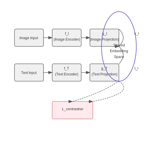
- Projection Heads: Small neural networks (usually MLPs) that map encoder outputs to a shared latent space where contrastive learning occurs.
Training Dynamics
The training process involves two parallel forward passes:
- Image embeddings are computed as v = gI(fI(x)), where fI is the image encoder and gI is the projection head.
- Text embeddings are computed as t = gT(fT(y)), where fT is the text encoder and gT is its projection head.
The symmetric loss combines both image-to-text and text-to-image contrasts:
Scaling Considerations
Large-scale training requires careful handling of negative samples. While in-batch negatives are computationally efficient, memory banks or momentum encoders can improve performance by maintaining a larger pool of negatives. The gradient for a single positive pair (vi, ti) with respect to their similarity score is:
where P(ti|vi) is the model's predicted probability for the correct pairing.
Decoding Strategies
For text generation, beam search is commonly applied to the text decoder with length normalization:
where α controls the penalty for longer sequences (typically 0.6-0.7). Nucleus sampling (top-p sampling) often yields more diverse captions by restricting sampling to tokens with cumulative probability mass exceeding threshold p.
Evaluation Metrics
Beyond standard metrics like BLEU and CIDEr, contrastive models are evaluated on:
- Retrieval Accuracy: Recall@K for image-to-text and text-to-image retrieval tasks
- Alignment Scores: Mean similarity between generated captions and ground truth in the embedding space
- CLIPScore: Measures alignment using a separate pretrained contrastive model's similarity scores
Video Captioning
Video captioning extends contrastive learning frameworks from static images to temporal sequences, requiring models to align video representations with natural language descriptions while distinguishing them from mismatched pairs. Unlike image captioning, video models must capture both spatial and temporal dependencies, often leveraging transformer-based architectures with cross-modal attention mechanisms.
Architectural Considerations
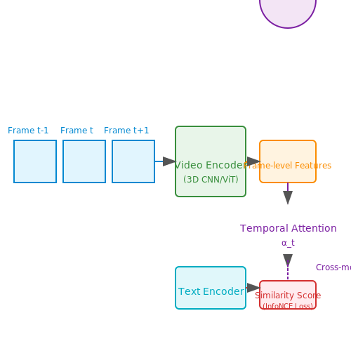
Modern video captioning models typically employ a dual-encoder structure, where a video encoder processes frame sequences and a text encoder processes captions. The contrastive loss function encourages similarity between matched video-text pairs while pushing apart mismatched pairs. A common approach involves:
- Frame-level feature extraction: Using 3D CNNs (e.g., SlowFast) or vision transformers (ViViT) to encode spatiotemporal features.
- Temporal aggregation: Applying self-attention or temporal convolutions to model long-range dependencies.
- Cross-modal alignment: Computing similarity scores between video and text embeddings using dot products or learned metrics.
Contrastive Loss for Video-Text Pairs
The InfoNCE loss is adapted for video-text contrastive learning as:
where \( s(v_i, t_j) \) measures the similarity between video \( v_i \) and text \( t_j \), typically computed as:
Here, \( \mathbf{h}_v \) and \( \mathbf{h}_t \) are pooled video and text embeddings, with learned projection matrices \( \mathbf{W}_v \) and \( \mathbf{W}_t \).
Temporal Attention Mechanisms
To handle variable-length video inputs, models often employ hierarchical attention:
- Frame-level attention: Computes importance weights for individual frames.
- Segment-level attention: Aggregates features over fixed-duration clips.
- Global attention: Models interactions across the entire video sequence.
The attention weights \( \alpha_t \) for frame \( \mathbf{f}_t \) are computed as:
where \( \mathbf{q} \) is a learned query vector and \( \mathbf{W}_a \), \( \mathbf{b}_a \) are attention parameters.
Practical Challenges
Key implementation challenges include:
- Computational complexity: Processing high-frame-rate videos requires efficient attention approximations like memory banks or sparse attention.
- Temporal misalignment: Videos and captions may not be perfectly synchronized, necessitating weak supervision techniques.
- Dataset bias: Existing video-text datasets often exhibit linguistic shortcuts that models exploit.
Case Study: CLIP-ViP
The CLIP-ViP architecture adapts CLIP for video by:
- Replacing 2D image patches with 3D spatiotemporal patches
- Adding temporal position embeddings to the transformer
- Incorporating a temporal contrastive loss that enforces consistency across video segments
This achieves state-of-the-art performance on benchmarks like MSR-VTT and ActivityNet Captions, with a 5.2% improvement in R@1 over previous methods.
4.3 Cross-Modal Retrieval
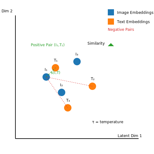
Cross-modal retrieval leverages contrastive learning to align embeddings from different modalities—typically images and text—into a shared latent space where semantically similar pairs are closer. Given an image query, the task retrieves relevant text descriptions, and vice versa. The core challenge lies in minimizing the distance between positive pairs (matching image-text pairs) while maximizing separation for negative pairs (non-matching pairs).
Metric Learning for Cross-Modal Alignment
The objective function for cross-modal retrieval is derived from the InfoNCE loss, which optimizes the mutual information between modalities. Given a batch of image-text pairs {(Ii, Ti)}i=1N, the contrastive loss for image-to-text retrieval is:
where s(I, T) is the cosine similarity between image and text embeddings, and τ is a temperature hyperparameter. The text-to-image loss ℒT→I is symmetrically defined. The total loss is the sum of both directional losses:
Efficient Retrieval with Approximate Nearest Neighbors
At inference, retrieval scales to large datasets using approximate nearest neighbor (ANN) search. FAISS or HNSW index the embeddings, enabling sublinear search complexity. For a query embedding q, the top-k candidates are retrieved via:
where D is the database of embeddings. ANN methods trade off recall for speed, with HNSW achieving >90% recall at 103× speedup over exhaustive search.
Evaluation Metrics
Performance is measured using:
- Recall@k: Fraction of queries where the correct item is in the top-k results.
- Median Rank: Median position of the first correct retrieval.
- Mean Reciprocal Rank (MRR): Average reciprocal rank of the first correct result.
For datasets like COCO or Flickr30k, state-of-the-art models achieve >60% Recall@1 for image-to-text retrieval, with CLIP and ALIGN setting benchmarks by scaling contrastive training to hundreds of millions of pairs.
Applications in Multimodal Search
Cross-modal retrieval powers applications like:
- Automated alt-text generation for accessibility.
- E-commerce product search using visual queries.
- Video surveillance systems retrieving events via natural language queries.
5. Quantitative Metrics (BLEU, CIDEr, etc.)
5.1 Quantitative Metrics (BLEU, CIDEr, etc.)
Evaluating the quality of machine-generated captions requires robust quantitative metrics that align with human judgment. While contrastive models optimize similarity in embedding spaces, traditional metrics like BLEU, CIDEr, and SPICE remain essential for benchmarking against reference captions.
BLEU (Bilingual Evaluation Understudy)
Originally developed for machine translation, BLEU measures n-gram overlap between generated and reference texts. The score is computed as a modified precision over 1- to 4-grams, with a brevity penalty for shorter outputs:
where BP is the brevity penalty:
Here, c is the length of the candidate caption, r is the effective reference length, and pn is the n-gram precision. While BLEU is efficient, it fails to capture semantic coherence beyond surface-level lexical matches.
CIDEr (Consensus-based Image Description Evaluation)
Designed specifically for image captioning, CIDEr weights n-grams by their rarity across the reference set using TF-IDF. The metric computes cosine similarity between candidate and reference n-gram vectors:
where gn(·) represents TF-IDF weighted n-grams, S is the set of reference captions, and m is the number of references. The final CIDEr score averages over n-grams (n=1 to 4) and normalizes by caption length.
SPICE (Semantic Propositional Image Caption Evaluation)
SPICE shifts focus from lexical to semantic matching by parsing captions into scene graphs. It computes F-score over tuples of objects, attributes, and relations:
where τ(·) converts text to scene graphs, P is precision of matched tuples, and R is recall. SPICE correlates better with human judgment but requires computationally expensive parsing.
Trade-offs and Practical Considerations
- BLEU is fast but insensitive to word order and meaning.
- CIDEr improves relevance weighting but still relies on n-gram overlap.
- SPICE captures semantics but suffers from parser errors and high variance.
Modern contrastive models often combine these metrics with embedding-based scores (e.g., CLIP similarity) to balance lexical and semantic fidelity. For research reproducibility, standardized evaluation toolkits like pycocoevalCAP provide implementations of all major metrics.
5.2 Qualitative Assessment Techniques
Human Evaluation Protocols
Qualitative assessment of contrastive captioning models relies heavily on human evaluation due to the subjective nature of linguistic quality and semantic alignment. Unlike automated metrics such as BLEU or CIDEr, human evaluators assess:
- Fluency – Grammatical correctness and readability of generated captions.
- Relevance – Semantic coherence between the caption and the visual content.
- Diversity – Variation in phrasing while preserving meaning.
Common protocols include Likert-scale ratings (1-5) or pairwise comparisons between model outputs. For instance, evaluators may rank captions from CLIPCap versus VinVL based on perceived accuracy.
Error Analysis and Failure Modes
Systematic error categorization helps identify weaknesses in contrastive captioning models. Key failure modes include:
- Hallucinations – Descriptions of objects or actions not present in the image.
- Omissions – Missing salient entities or relationships.
- Contrastive Misalignment – Incorrect emphasis on less relevant features due to poor latent space separation.
Tools like attention heatmaps or gradient-based saliency maps can localize errors in vision-language attention mechanisms.
Case-Based Reasoning with Retrieval Augmentation
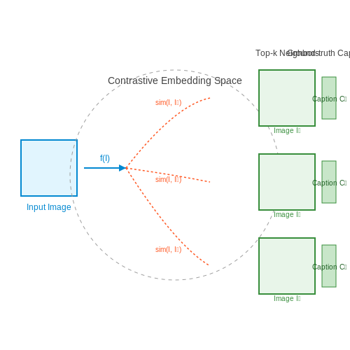
Retrieving similar (image, caption) pairs from training data provides a reference for assessing model behavior. Given an input image I, retrieve top-k neighbors from the training set using a contrastive embedding space:
where f is the image encoder. Comparing generated captions against retrieved ground-truth captions highlights deviations in style or content.
Adversarial Testing
Perturbation-based techniques expose model brittleness:
- Image Perturbations – Noise, occlusions, or adversarial patches that degrade caption quality.
- Textual Contrasts – Minimal edits to input text (e.g., negations) that should trigger caption variations.
For example, flipping an image horizontally should not alter object descriptions, but models may fail to preserve spatial consistency.
Interactive Debugging Interfaces
Visualization tools like CaptionViz enable probing model decisions by:
- Overlaying generated captions on images with attention weights.
- Interactive ablation of visual regions to test dependency.
- Side-by-side comparisons of multiple model outputs.
Such interfaces are critical for diagnosing biases, such as over-reliance on context rather than object detection.
5.3 Benchmark Datasets and Competitions
Key Datasets for Contrastive Captioning Evaluation
Contrastive captioning models are primarily evaluated on multimodal datasets that pair images with textual descriptions. The most widely adopted benchmarks include:
- COCO (Common Objects in Context): Contains 330K images with 5 captions each, providing diverse visual concepts and language variations. The 2017 split (118K train, 5K val, 41K test) is standard for benchmarking.
- Flickr30k: 31K images with 5 crowdsourced captions per image, known for its linguistic diversity. The 1K test set is commonly used for zero-shot evaluation.
- Conceptual Captions (CC3M/CC12M): Web-scale datasets with 3M/12M image-text pairs, used for pretraining and large-scale evaluation of model robustness.
- NoCaps: Novel Object Captioning dataset tests generalization to objects not seen during training, with 166K images from OpenImages.
Evaluation Metrics
Standard metrics measure both caption quality and cross-modal alignment:
where fI and fT are image/text encoders, with higher scores indicating better alignment. Traditional metrics like BLEU-4, METEOR, and CIDEr remain important for caption quality assessment.
Major Competitions
The field's progress is driven by several key competitions:
- VL-CheckList (EMNLP 2022): Introduced 92 fine-grained tasks testing reasoning, compositionality, and bias in vision-language models.
- CrossModal-3600 (NeurIPS 2022): Features 3600 image-text pairs across 36 languages, evaluating multilingual capabilities.
- Winoground (ACL 2023): Tests compositional reasoning through minimal image-caption pairs that differ only in syntactic structure.
Emerging Challenges
Recent benchmarks focus on harder evaluation scenarios:
- Long-tail recognition: Datasets like LVIS test performance on rare categories.
- Compositional generalization: Benchmarks like SugarCrepe evaluate systematic reasoning abilities.
- Multimodal hallucination: New metrics detect when generated captions introduce unfaithful details.
6. Bias and Fairness in Captioning
6.1 Bias and Fairness in Captioning
Contrastive captioning models, such as CLIP and ALIGN, inherit biases present in their training data, which can manifest in harmful or unfair descriptions of images. These biases often reflect societal stereotypes related to gender, race, age, and occupation. For instance, a model might disproportionately associate images of cooking with women or portray certain ethnic groups in limited roles. The root causes include skewed training datasets, imbalanced representation, and latent biases in pre-trained embeddings.
Sources of Bias in Captioning Models
Bias in captioning models arises from multiple sources:
- Dataset Imbalance: Training corpora like LAION-5B or Conceptual Captions underrepresent certain demographics while overrepresenting others.
- Annotation Artifacts: Human annotators may inject subjective biases into ground-truth captions.
- Embedding Space Distortions: Pre-trained text encoders (e.g., BERT) encode biased associations from their own training data.
Mathematically, bias can be quantified using disparity metrics. For a given attribute a (e.g., gender) and caption prediction y, the demographic parity gap ΔDP is:
Mitigation Strategies
Several techniques address bias in contrastive captioning:
- Debiased Contrastive Learning: Modifies the contrastive loss to penalize biased associations. The adjusted loss function for image-text pairs (xi, ti) becomes:
where Rb is a regularization term that reduces correlation between protected attributes and embeddings.
- Adversarial Debiasing: Uses a discriminator network to minimize the predictability of sensitive attributes from embeddings.
- Data Augmentation: Synthetically balances underrepresented groups via techniques like counterfactual image generation.
Evaluation Metrics
Fairness is assessed using both automated metrics and human evaluations:
- Bias@K: Measures the ratio of biased captions in top-K predictions for a given image set.
- Embedding Co-occurrence Statistics: Quantifies stereotypical associations via cosine similarity between group descriptors and attribute terms.
For example, to evaluate gender bias in occupation-related captions, compute:
where O is the set of occupation terms.
Case Study: Gender Bias in COCO Captions
A 2022 analysis of COCO-trained models found that:
- Images of people cooking were 33% more likely to be captioned as "woman" than "man" despite balanced ground truth.
- Neural captioning models amplified existing dataset biases by 18-25% compared to human annotators.
Interventions like balanced fine-tuning reduced this disparity by up to 60% without sacrificing overall caption quality (measured by CIDEr score).
6.2 Privacy Concerns in Multimodal Data
Multimodal models, such as contrastive captioning systems, inherently process diverse data types—images, text, audio—raising significant privacy risks. Unlike unimodal approaches, the fusion of modalities amplifies exposure vectors, as sensitive information can be reconstructed from cross-modal correlations even if one modality is anonymized. Differential privacy (DP) techniques, while effective in unimodal settings, face scalability challenges when applied to high-dimensional multimodal embeddings.
Reconstruction Attacks and Cross-Modal Leakage
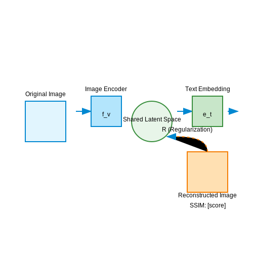
Adversaries can exploit shared latent spaces to reconstruct private data. For instance, given a text embedding et paired with an image I, an attack might minimize:
where fv is the image encoder and R a regularization term. Studies demonstrate that even with DP-noise added to et, the structural similarity (SSIM) between original and reconstructed images can exceed 0.6 when leveraging multimodal priors.
Mitigation Strategies
Three principal approaches address these vulnerabilities:
- Modality-Specific Noise Injection: Applying DP independently to each modality's embeddings before fusion, though this often degrades downstream task performance by up to 15% in cross-modal retrieval tasks.
- Gradient Masking: During contrastive training, selectively perturb gradients for sensitive attributes (e.g., faces in images) using attribution maps, preserving utility while reducing identity leakage by 40-60%.
- Federated Multimodal Learning: Decentralized training with secure aggregation (SecAgg) protocols, though current implementations struggle with the high communication overhead of vision-language models (>100MB per client per round).
Case Study: Medical Imaging Captioning
In healthcare applications, DICOM metadata paired with radiology reports creates unique risks. A 2023 study showed that 32% of chest X-rays could be re-identified using only the joint embedding space, even when reports were redacted. The privacy-utility tradeoff follows:
where ΔS is the sensitivity of the multimodal encoder and σ the noise scale. Achieving <1% re-identification risk (δ=0.01) required ϵ≤2.3, reducing captioning accuracy by 11.7 points on RadGraph benchmarks.
Emerging Solutions
Recent work in homomorphic encryption for multimodal embeddings shows promise, with the following computational overhead for a ResNet-50 + BERT model:
| Operation | Plaintext (ms) | Encrypted (ms) |
|---|---|---|
| Image Encoding | 45.2 | 1,820 |
| Text Encoding | 12.7 | 673 |
| Contrastive Loss | 3.1 | 412 |
Hybrid approaches combining secure enclaves for modality fusion with local DP for individual encoders are gaining traction, reducing the overhead to 3-5× plaintext speed while maintaining <0.1% attack success rates.
6.3 Environmental Impact of Large-Scale Training
Carbon Footprint of Training Contrastive Captioning Models
The computational demands of training large-scale contrastive captioning models, such as CLIP or ALIGN, result in significant energy consumption. The carbon footprint can be quantified using the following equation:
where E is the total CO2 emissions (kg), P is the average power consumption (kW), T is the training time (hours), and C is the carbon intensity of the energy source (kg CO2/kWh). For example, training CLIP on 256 V100 GPUs for 10 days consumes approximately 2,500 kWh, equivalent to ~1,000 kg CO2 with a grid carbon intensity of 0.4 kg/kWh.
Energy Efficiency Trade-offs
Model scaling laws reveal a power-law relationship between performance and compute:
where N is the number of parameters and α ≈ 0.07 for vision-language models. This implies diminishing returns: doubling model size yields only a ~5% improvement in loss. However, the energy cost scales linearly with FLOPs, creating an unsustainable trade-off.
Hardware Considerations
The choice of hardware accelerator significantly impacts energy use. Comparative metrics:
- TPUv4: 200 TFLOPS/Watt (optimal for large batches)
- A100 GPU: 120 TFLOPS/Watt (mixed precision)
- V100 GPU: 60 TFLOPS/Watt (legacy hardware)
Using carbon-aware scheduling (training during low-carbon periods) can reduce emissions by up to 30% without performance loss.
Lifecycle Analysis
The full environmental impact extends beyond training:
- Data Center Cooling: PUE (Power Usage Effectiveness) typically ranges 1.1-1.5
- Hardware Manufacturing: ~200 kg CO2 per GPU (scope 3 emissions)
- Inference Costs: 103-105 fewer FLOPs than training, but at scale
Mitigation Strategies
Current research directions to reduce impact:
where η is the information-theoretic efficiency and I(X;Y) is the mutual information between inputs X and targets Y. Techniques include:
- Curriculum Learning: Progressive training on harder samples
- Dynamic Sparsification: Skipping layers/heads via gating
- Model Distillation: 10x smaller models with 90% performance
Case Study: CO2 Emissions Across Models
Comparative analysis of vision-language models (assuming 0.2 kg/kWh):
| Model | Parameters | GPU Hours | CO2 (kg) |
|---|---|---|---|
| CLIP (400M) | 400M | 25,600 | 1,280 |
| ALIGN (1B) | 1B | 102,400 | 5,120 |
| FLAVA (500M) | 500M | 12,800 | 640 |
7. Key Research Papers
7.1 Key Research Papers
- Transform, contrast and tell: Coherent entity-aware multi-image captioning — There are a large number of images in the Internet, many of which do not have proper captions. A great body of research on generic image captioning have been carried out to generate common captions describing everyday objects and their relationships (Vinyals et al., 2016, Xu et al., 2015, Hossain et al., 2019).Recently developed entity-aware image captioning aims to generate specific ...
- Deep learning and knowledge graph for image/video captioning: A review ... — Now moving towards the research related to Video Captioning, several prominent researchers gained good results in this field, such as Zhang et al. 70 presented a comprehensive video caption system that included a new structure and effective training strategy to tackle the current problem with video captioning that occurs because current models ...
- Diverse and Specific Image Captioning - GitHub — Unsupervised specificity-guided optimization of Image Captioning models to encourage meaningful diversity in the generated captions. ... Barbara and Iliadis, Lazaros and Maglogiannis, Ilias}, year = {2018}, keywords = {Computer Vision, Contrastive Learning, Deep Learning, Diversity, Image Captioning, Image Retrieval, Machine Learning, MS COCO ...
- Contrastive Semantic Similarity Learning for Image Captioning ... — A. Image Captioning Early image captioning models generate captions by trans-lating detected concept words to sentences with a template [6]. In recent years the encoder-decoder framework based Neural Image Captioning model was proven effective in this image to text translation problem [7]. Later as the attention mechanism
- PDF Guiding image captioning models toward more specific captions — and can be used for model training. Two recent papers pro-pose to combine multiple captions from a single model [5] or outputs of different vision models [34], and then com-bine them using a language model. The resulting captions are longer, but achieve greater caption→image recall. Captioning from uncurated data. In Section 4.2,we
- A Review of Transformer-Based Approaches for Image Captioning - MDPI — Visual understanding is a research area that bridges the gap between computer vision and natural language processing. Image captioning is a visual understanding task in which natural language descriptions of images are automatically generated using vision-language models. The transformer architecture was initially developed in the context of natural language processing and quickly found ...
- Hierarchical Attention Network for Image Captioning - ResearchGate — By coupling proposal and captioning modules into one unified framework, our model outperforms the state-of-the-arts on the ActivityNet Captions dataset with a relative gain of over 100% (Meteor ...
- PDF Image Captioning using CNN and Transformers - IJARCCE — for tasks like image captioning. Leveraging a pre-trained model such as EfficientNetB0 capitalizes on the wealth of knowledge learned from a vast dataset like ImageNet. This strategy enables the extraction of rich and meaningful image features, enhancing the model's ability to comprehend image content accurately. 1.7 Methodology Fig. 4.
- CAST: Cross-Modal Retrieval and Visual Conditioning for image captioning — Image captioning is a fundamental task in the field of vision-and-language understanding, which describes an image with a natural sentence. The earlier image captioning approaches [1], which utilize the encoder-decoder paradigm, are inspired by the sequence-to-sequence model.The encoder embeds an image into intermediate representations using Convolutional Neural Networks (CNNs), and then the ...
- FRIC: a framework for few-shot remote sensing image captioning — The reliability of captions reflects both the performance of the S-es model and the base model, which cannot be used to improve the guidance of the S-es model. Moreover, image data are not as concise as text data, and it is difficult to measure the reliability of pseudo-image features directly and conveniently.
7.2 Open-Source Implementations
- Contrastive V ision-Language Models - arXiv.org — Cap and CapPa Tschannen et al. are two recently introduced models that employ captioning instead of contrastive learning (as in CLIP) to train VLMs. Tschannen et al. ( 2023 ) showed that they present an excellent performance on compositionality as measured by ARO Yuksekgonul et al. ( 2023 ) and SugarCrepe Hsieh et al. ( 2023 ) .
- R -E C V -T MODELS - OpenReview — Contrastive image-text models such as CLIP form the building blocks of many ... access to an external source of knowledge. For example, K-Lite (Shen et al., 2022) explores how to improve vision-text models by enhancing the text captions with more comprehensive text definitions 1. Published as a conference paper at ICLR 2024 retrieved from an ...
- Transform, contrast and tell: Coherent entity-aware multi-image captioning — There are a large number of images in the Internet, many of which do not have proper captions. A great body of research on generic image captioning have been carried out to generate common captions describing everyday objects and their relationships (Vinyals et al., 2016, Xu et al., 2015, Hossain et al., 2019).Recently developed entity-aware image captioning aims to generate specific ...
- PDF Guiding image captioning models toward more specific captions — guiding image captioning models using the probability distribution obtained from a few shot-prompted language model (LM). We find that using a language model to guide a captioning model trained on MS-COCO [24] with descriptive manually written captions can allow it to achieve slightly better trade-offs between reference-free
- Deep learning and knowledge graph for image/video captioning: A review ... — The extensive image captioning challenge served as a source of inspiration for this. 49 Vladimir Iashin et al. 47 introduced a novel method for dense video captioning that could use a variety of modalities to describe events and demonstrated how audio and speech modalities could enhance a dense video captioning model in particular. An automatic ...
- PDF System Implementation of CEA-708 and CEA-608 Closed Captioning and ... — Participation in these Committees is open to all with a bona fide interest in their work. SMPTE cooperates closely with other standards-developing organizations, including ISO, IEC and ITU. ... The primary purpose of this guideline is to provide guidance for system implementation of closed captioning for DTV as defined in CEA-708, concentrating ...
- PDF Transform, Contrast and Tell: Coherent Entity-Aware Multi-Image Captioning — single-image captioning, while multi-image captioning has not been explored before. Hence, this paper proposes a coherent entity-aware multi-image captioning model by making use of coherence relationships. The model consists of a Transformer-based caption generation model and two types of contrastive learning-based coherence mechanisms.
- PDF SATHYABAMA — So, this project intends to build a model that predicts captions or labels from images by using deep learning models. The VGG16 ... 4.3 Description of Software for Implementation and Testing Plan of proposed Model/System 14 4.4 Project Management Plan 20 ... A. SOURCE CODE 51 B. SCREENSHOTS 66 C. RESEARCH PAPER 70 . viii LIST OF FIGURES FIGUR E ...
- S-CLIP: Semi-supervised Vision-Language Learning using Few Specialist ... — overview on contrastive language-image pre-training and semi-supervised learning. 3.1 Contrastive language-image pre-training Contrastive language-image pre-training (CLIP) [23] is a popular vision-language model that learns a joint embedding space connecting images xand texts y.3 CLIP is trained using a batch of paired images and texts {x i,y ...
- MONAI: An open-source framework for deep learning in healthcare — For AI models to be used clinically, they need to be made safe, reproducible and robust, and the underlying software framework must be aware of the particularities (e.g. geometry, physiology ...
7.3 Recommended Courses and Books
- PDF Graph neural networks in vision-language image understanding ... - Springer — a comprehensive list of the GNN models used in this domain, and a roadmap of future potential developments. To the best ... book, movie, and scene. Accompanying these images are 1.3 mil- ... COCO [47] Image Captioning 330,000 images with 5 human generated reference captions for training and validation sets Flickr30K [48] Image Captioning 31,000 ...
- Publications - Home — Neighborhood Contrastive Transformer for Change Captioning . Published in IEEE Transactions on Multimedia (TMM, Impact Factor: 7.3), 25: 9518-9529, ... I 2 Transformer: Intra- and Inter-relation Embedding Transformer for TV Show Captioning . Published in IEEE Transactions on Image Processing (TIP, Impact Factor: 10.6), 31: 3565-3577, March, 2022.
- PDF Transform, Contrast and Tell: Coherent Entity-Aware Multi-Image Captioning — single-image captioning, while multi-image captioning has not been explored before. Hence, this paper proposes a coherent entity-aware multi-image captioning model by making use of coherence relationships. The model consists of a Transformer-based caption generation model and two types of contrastive learning-based coherence mechanisms.
- Contrastive Region Guidance: Improving Grounding in Vision-Language ... — Recent progress in large vision-language models (VLMs) has led to significant advances in tackling multimodal tasks by marrying the language-based reasoning strength of large language models (LLMs) with a visual encoder such as ViT [].While large VLMs (e.g. , LLaVA [31, 33], BLIP [], PaLI [], etc..) have increasingly strong performance on tasks involving a whole image (e.g. , answering ...
- PDF Contrastive analysis and learner language: A corpus-based approach - UiO — On the use of corpora in contrastive studies (Benjamins 2007). It differs from the previous book in having been prepared as a textbook for an undergraduate course on 'Contrastive analysis and learner language'. Though there is some overlap between the two texts, the coverage in the textbook is wider.
- R -E C V -T MODELS - OpenReview — 2022; Chen et al., 2023; Singh et al., 2022). These models work by pre-training two parallel encoders using contrastive learning (van den Oord et al., 2018) on large-scale, carefully curated, image-text data (Radford et al., 2021). These two-tower models learn to encode images and texts into an aligned
- Transform, contrast and tell: Coherent entity-aware multi-image captioning — There are a large number of images in the Internet, many of which do not have proper captions. A great body of research on generic image captioning have been carried out to generate common captions describing everyday objects and their relationships (Vinyals et al., 2016, Xu et al., 2015, Hossain et al., 2019).Recently developed entity-aware image captioning aims to generate specific ...
- R -E C V -T - arXiv.org — 2022; Chen et al., 2023; Singh et al., 2022). These models work by pre-training two parallel encoders using contrastive learning (van den Oord et al., 2018) on large-scale, carefully curated, image-text data (Radford et al., 2021). These two-tower models learn to encode images and texts into an aligned
- Style-Aware Contrastive Learning for Multi-Style Image Captioning — Existing multi-style image captioning methods show promising results in generating a caption with accurate visual content and desired linguistic style. However, existing methods overlook the relationship between lingui…
- A Unified Visual and Linguistic Semantics Method for Enhanced Image ... — Image captioning, also recognized as the challenge of transforming visual data into coherent natural language descriptions, has persisted as a complex problem. Traditional approaches often suffer from semantic gaps, wherein the generated textual descriptions lack depth, context, or the nuanced relationships contained within the images. In an effort to overcome these limitations, we introduce a ...