Video Captioning with Transformers
1. Problem Definition and Applications
1.1 Problem Definition and Applications
Video captioning is the task of generating natural language descriptions for video content, combining computer vision and natural language processing. Given an input video sequence V = {v1, v2, ..., vT} consisting of T frames, the objective is to produce a textual output sequence S = {s1, s2, ..., sN} that accurately describes the visual content, actions, and context.
Mathematical Formulation
The problem can be framed as a sequence-to-sequence learning task, where the model learns a mapping f: V → S. The optimal caption S* maximizes the conditional probability:
where θ represents the model parameters. Using the chain rule, this decomposes into:
Key Challenges
- Temporal modeling: Capturing long-range dependencies across video frames requires effective temporal feature aggregation.
- Multimodal alignment: The model must learn joint representations between visual features and linguistic semantics.
- Context preservation: Maintaining coherence across generated words while avoiding repetition or hallucination.
Transformer Architecture Adaptation
Standard transformer architectures require three key modifications for video captioning:
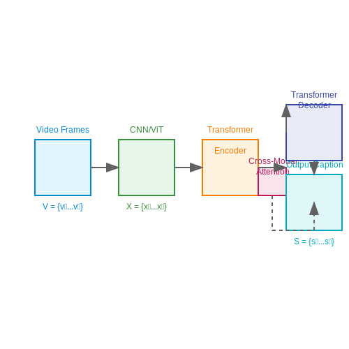
- Visual feature extraction: A CNN or ViT backbone encodes frame-level features X = {x1, ..., xT}.
- Spatiotemporal attention: Self-attention layers process both intra-frame and inter-frame relationships.
- Cross-modal decoder: Text generation attends to visual features through encoder-decoder attention.
Applications
Video captioning enables numerous real-world applications:
- Accessibility: Automatic descriptions for visually impaired users.
- Video retrieval: Semantic search through large video archives.
- Surveillance: Automated logging of security footage events.
- Education: Generating lecture summaries from recorded classes.
Evaluation Metrics
Standard benchmarks use:
where BP is the brevity penalty and pn are n-gram precisions. Additional metrics include METEOR, CIDEr, and SPICE, which incorporate semantic similarity measures beyond lexical overlap.
Key Challenges in Video Captioning
Multimodal Feature Alignment
Video captioning requires precise alignment between visual and textual modalities. Unlike static images, videos contain temporal dynamics, making it challenging to synchronize visual features with corresponding linguistic descriptions. The transformer architecture, while powerful, must handle varying frame rates and scene transitions. Misalignment often leads to captions that are either too generic or temporally inconsistent.Long-Range Temporal Dependencies
Videos often contain actions or events that span multiple seconds or minutes. Capturing these long-range dependencies is non-trivial, as standard attention mechanisms in transformers may struggle with computational inefficiency when processing high-frame-rate inputs. Hierarchical attention or memory-augmented networks are often employed to mitigate this issue.Semantic Granularity
Generating captions with the appropriate level of detail—ranging from coarse scene descriptions to fine-grained action annotations—is a persistent challenge. Overly detailed captions may introduce noise, while overly simplistic ones fail to convey critical information. This trade-off is often addressed through reinforcement learning or multi-task learning objectives.Dataset Bias and Generalization
Most video captioning models are trained on domain-specific datasets (e.g., sports, cooking), leading to biased performance when applied to unseen domains. Zero-shot or few-shot learning techniques are increasingly explored to improve generalization, but they require careful handling of out-of-distribution samples.Real-Time Processing Constraints
Deploying video captioning systems in real-world applications demands low-latency inference. However, transformer-based models are computationally intensive, especially for high-resolution videos. Optimizations such as model pruning, quantization, or efficient attention variants (e.g., Linformer, Performer) are critical for practical deployment.Evaluation Metrics and Human Consensus
Traditional metrics like BLEU, METEOR, and CIDEr often fail to capture semantic correctness or temporal coherence. Human evaluation remains the gold standard but is expensive and subjective. Recent work explores adversarial evaluation or learned metrics to bridge this gap.Ethical and Privacy Concerns
Video captioning systems may inadvertently generate biased or offensive captions due to training data artifacts. Additionally, processing real-world videos raises privacy concerns, particularly in surveillance or healthcare applications. Techniques like differential privacy and fairness-aware training are emerging as potential solutions.1.3 Traditional Approaches vs. Transformer-Based Methods
Traditional Video Captioning Methods
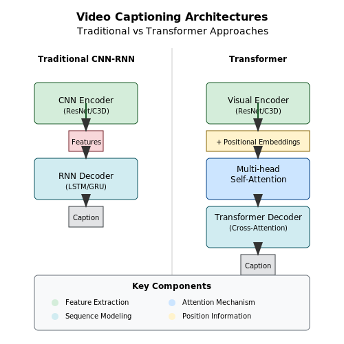
Early video captioning systems relied on a two-stage pipeline: feature extraction followed by sequence generation. Convolutional Neural Networks (CNNs) such as ResNet, C3D, or I3D were used to encode spatial and temporal features from video frames. These features were then fed into Recurrent Neural Networks (RNNs), typically LSTMs or GRUs, to generate descriptive captions. The probability of generating a word sequence y given video features v was modeled as:
This approach suffered from several limitations:
- Information bottleneck: The CNN encoder compressed all temporal information into a fixed-length vector, losing fine-grained motion details.
- Exposure bias: During training, the model received ground truth words as input, but at inference, it relied on its own predictions, leading to error accumulation.
- Long-range dependencies: RNNs struggled to capture relationships between distant visual events and their textual descriptions.
Transformer-Based Paradigm Shift
Transformer architectures revolutionized video captioning by replacing the CNN-RNN pipeline with self-attention mechanisms. The key innovations include:
Where Q, K, and V represent queries, keys, and values respectively, and dk is the dimension of the keys. This allows:
- Direct modeling of all pairwise interactions between visual features and words
- Parallel processing of the entire sequence during training
- Multi-head attention to jointly attend to different representation subspaces
Architectural Comparison
The transformer-based video captioning framework typically consists of:
- Visual encoder: A spatiotemporal transformer that processes raw frames or clip features
- Text decoder: A language model with masked self-attention and cross-attention to visual features
- Positional embeddings: To maintain temporal ordering without recurrence
where X represents all encoder states and xt is the current decoder state. This architecture achieves superior performance through:
- End-to-end training of visual and linguistic components
- Dynamic attention that adapts to different video regions
- Scalability to longer sequences through parallel computation
Performance Metrics and Trade-offs
Quantitative comparisons on benchmark datasets (MSVD, MSR-VTT) show transformer-based methods outperform traditional approaches by significant margins:
| Method | BLEU-4 | METEOR | CIDEr |
|---|---|---|---|
| LSTM-YT | 33.3 | 29.1 | 51.7 |
| S2VT | 36.8 | 30.8 | 55.3 |
| Vanilla Transformer | 42.1 | 33.5 | 61.2 |
| MART | 45.7 | 35.1 | 65.8 |
The performance gains come with increased computational complexity, where the self-attention mechanism scales quadratically with sequence length. Recent optimizations like memory-efficient attention and sparse transformers help mitigate this cost.
2. Overview of Transformer Models
Overview of Transformer Models
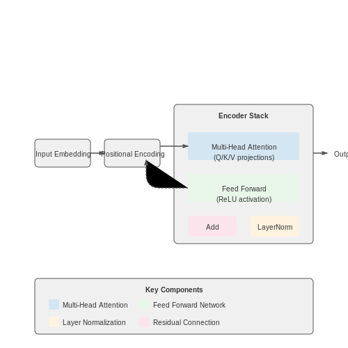
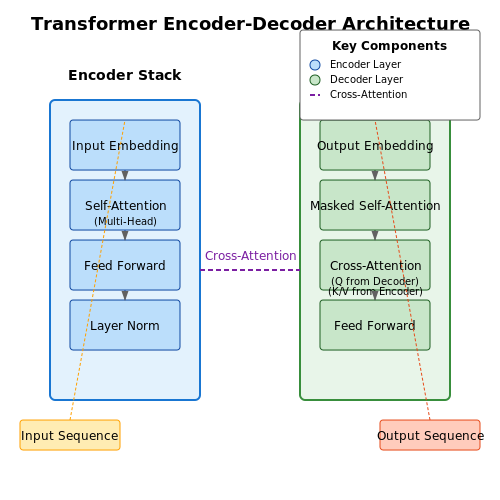
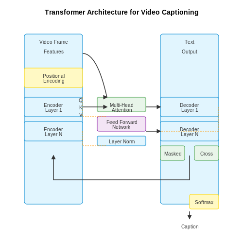
Transformer models, introduced by Vaswani et al. in 2017, revolutionized sequence modeling by replacing recurrent and convolutional architectures with self-attention mechanisms. The core innovation lies in the ability to capture long-range dependencies without sequential processing, enabling parallelization and improved scalability. The architecture consists of stacked encoder and decoder layers, each employing multi-head attention, position-wise feed-forward networks, and residual connections with layer normalization.
Self-Attention Mechanism
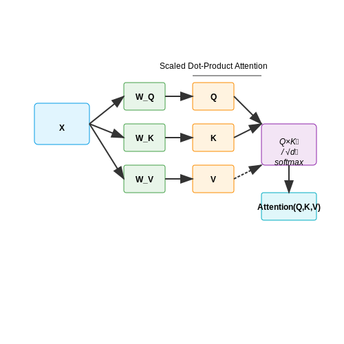
The self-attention mechanism computes a weighted sum of input representations, where weights are derived from pairwise similarity between elements. Given an input sequence X ∈ ℝn×d, the queries (Q), keys (K), and values (V) are computed as linear transformations:
where WQ, WK, WV ∈ ℝd×dk are learnable weight matrices. The attention scores are computed as:
The scaling factor √dk prevents gradient vanishing in high-dimensional spaces. Multi-head attention extends this by projecting Q, K, V into h subspaces, allowing the model to attend to different representation subspaces simultaneously.
Positional Encoding
Since transformers lack inherent sequential processing, positional encodings inject order information into the input embeddings. For position pos and dimension i, the encoding uses sinusoidal functions:
This choice allows the model to generalize to unseen sequence lengths better than learned positional embeddings.
Encoder-Decoder Architecture
The encoder processes input sequences through N identical layers, each containing:
- A multi-head self-attention sublayer
- A position-wise feed-forward network (FFN) with ReLU activation: FFN(x) = max(0, xW1 + b1)W2 + b2
- Residual connections and layer normalization
The decoder extends this with an additional cross-attention mechanism between encoder outputs and decoder inputs, enabling sequence-to-sequence tasks like video captioning. Masked self-attention in the decoder prevents information leakage from future positions during training.
Key Advantages for Video Captioning
Transformers excel at video captioning due to:
- Parallel processing of frame features, unlike RNNs' sequential bottleneck
- Global context modeling through attention across all frames
- Multi-modal alignment between visual features and text tokens via cross-attention
Modern video transformers often employ hybrid architectures, where 3D CNNs or ViTs extract spatial-temporal features, followed by transformer decoders for language generation. The attention mechanism's flexibility allows modeling complex interactions between visual concepts and linguistic structure.
2.2 Adapting Transformers for Video Input
Transformers, originally designed for sequential data like text, require significant architectural modifications to handle the high-dimensional spatiotemporal nature of video data. The primary challenge lies in efficiently modeling both spatial and temporal dependencies while maintaining computational tractability.
Video Tokenization Strategies
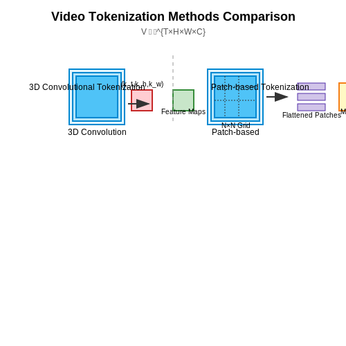
Unlike text tokenization which operates on discrete word units, video inputs require continuous feature extraction. Two dominant approaches exist:
- 3D Convolutional Tokenization: Uses 3D CNNs (e.g., SlowFast, I3D) to extract spatiotemporal features from video cubes. For a video clip V ∈ ℝT×H×W×C, the 3D convolution operation with kernel size (kt, kh, kw) produces tokens:
- Patch-based Tokenization: Inspired by Vision Transformers (ViT), this method divides each frame into N × N patches which are flattened and projected:
where E is the patch embedding matrix and epos encodes spatiotemporal position.
Temporal Attention Mechanisms
Standard self-attention computes relationships between all spatiotemporal tokens, resulting in O(N2T2) complexity for N spatial tokens and T frames. Several efficient variants have emerged:
Factorized Attention
Decomposes the full attention into separate spatial and temporal components:
Local Window Attention
Restricts attention to local spatiotemporal neighborhoods, reducing memory requirements while preserving local motion patterns. For a window size w, complexity drops to O(NTw2).
Positional Encoding for Video
Video transformers require joint spatiotemporal position encoding. A common approach combines 2D spatial encoding with temporal encoding:
where PExy uses standard 2D sinusoidal encoding and PEt employs learned temporal embeddings.
Architectural Variants
Several transformer architectures have demonstrated success in video captioning:
- TimeSformer: Uses divided space-time attention with factorized attention blocks
- ViViT: Extends ViT with tubelet embedding and temporal transformer layers
- Motionformer: Incorporates optical flow as an additional motion modality
where ft represents optical flow features and ∥ denotes concatenation.
Memory Optimization Techniques
Processing long video sequences requires specialized memory management:
- Gradient Checkpointing: Reduces memory by recomputing activations during backward pass
- Mixed-Precision Training: Uses FP16 for activations while maintaining FP32 master weights
- Sequence Chunking: Processes long videos as overlapping segments with attention masking
2.3 Attention Mechanisms in Video Processing
Core Principles of Attention in Video
Attention mechanisms enable models to dynamically focus on relevant spatiotemporal regions within video frames while suppressing irrelevant information. Unlike static image processing, video introduces an additional temporal dimension, requiring attention to operate across both space and time. The fundamental operation computes a weighted sum of features, where weights are learned based on contextual relevance.
Here, Q (queries), K (keys), and V (values) are derived from the input video features. The scaling factor √dk prevents gradient saturation in the softmax.
Spatiotemporal Attention Variants
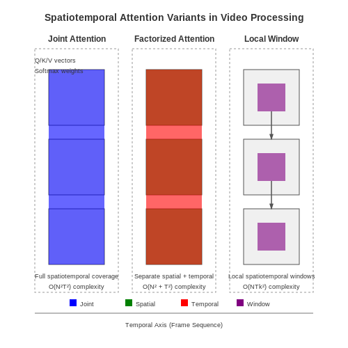
Video-specific attention extends standard self-attention with three primary variants:
- Joint Spatiotemporal Attention: Computes attention across all spatial and temporal positions simultaneously. This is computationally expensive but captures full dependencies.
- Factorized Attention: Separates spatial and temporal attention layers, reducing complexity from O(n2t2) to O(n2 + t2) for n spatial and t temporal positions.
- Local Window Attention: Restricts attention to local neighborhoods in space-time, trading off some global context for efficiency.
Efficient Video Attention Architectures
Recent work optimizes video attention through:
- Memory-efficient attention: Approximates full attention using techniques like kernel methods or low-rank projections.
- Hierarchical attention: Processes video at multiple temporal resolutions, applying coarse attention first followed by refinement.
- Deformable attention: Learns dynamic sampling locations rather than fixed grids, better handling motion.
where Δpk are learned offsets and wk are attention weights for K sampling points.
Case Study: Video Captioning with Attention
In video captioning, attention mechanisms:
- Align generated words with relevant visual regions (e.g., focusing on a "dog" when describing it).
- Track objects across frames via temporal attention.
- Use cross-modal attention between visual features and text embeddings.
Modern architectures like Vanilla Transformer, TimeSformer, and VidTr demonstrate these principles with varying attention configurations.
3. Video Feature Extraction Techniques
3.1 Video Feature Extraction Techniques
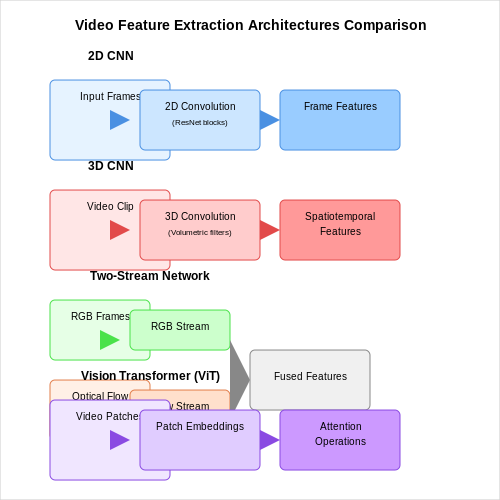
Video captioning requires robust spatiotemporal feature extraction to encode both visual appearance and motion dynamics. Modern approaches leverage deep convolutional networks, 3D convolutions, or hybrid architectures to capture hierarchical representations from raw video frames.
2D CNN-Based Frame-Level Features
Pretrained image classification networks like ResNet, Inception, or EfficientNet extract discriminative spatial features from individual frames. Given an input frame It at time t, a CNN backbone produces a feature map:
where H, W, and D denote height, width, and channel dimensions. Global average pooling often reduces this to a fixed-length vector ft ∈ ℝD. While computationally efficient, this approach ignores temporal dependencies between frames.
3D Convolutional Networks
3D CNNs explicitly model spatiotemporal structure by applying volumetric filters across frame sequences. For a video clip V = (I1,...,IT), a 3D convolution operates on stacked frames:
where W is the 3D kernel spanning spatial dimensions (l,m) and temporal dimension n. Architectures like C3D, I3D, and SlowFast employ 3D convolutions in deeper networks, with I3D inflating 2D ImageNet-pretrained weights into 3D for improved initialization.
Two-Stream Networks
Two-stream architectures fuse RGB appearance features with optical flow motion representations. The spatial stream processes raw frames, while the temporal stream takes stacked flow fields as input. Late fusion combines both streams:
where ⊕ denotes concatenation and ϕ is a fusion operator (e.g., MLP or attention). This approach captures complementary information but requires precomputing optical flow.
Transformer-Based Feature Extraction
Vision Transformers (ViTs) adapted for video divide input into spatiotemporal patches. For a sequence of N patches per frame across T timesteps, patch embeddings are computed as:
where pi,j is the (i,j)-th patch, E is an embedding matrix, and epos adds positional information. Models like TimeSformer apply self-attention across space and time, while ViViT uses factorized attention for efficiency.
Self-Supervised Pretraining
Contrastive methods like MoCo or SimCLR learn representations without manual labels by maximizing agreement between differently augmented views of the same video. Given two augmented clips Vq and Vk, the InfoNCE loss encourages feature similarity:
where τ is a temperature parameter and k+ is the positive sample. This yields features transferable to downstream captioning tasks with limited labeled data.
Text Tokenization and Vocabulary Building
Text tokenization is the process of breaking down raw text into smaller units called tokens, which serve as the atomic elements for downstream processing in transformer-based video captioning models. The choice of tokenization strategy directly impacts model performance, computational efficiency, and generalization capability.
Subword Tokenization Algorithms
Modern transformer architectures predominantly use subword tokenization to balance vocabulary size with semantic granularity. Three principal algorithms dominate this space:
- Byte Pair Encoding (BPE): A data compression-derived method that iteratively merges frequent character pairs. Given a corpus with initial vocabulary V (all unique characters) and merge operations count k, the algorithm computes:
where counts are computed over the training corpus. BPE continues merging until the vocabulary reaches target size |V| + k.
- WordPiece: Similar to BPE but uses likelihood maximization rather than frequency counts. The merge criterion becomes:
- Unigram Language Model: Starts with a large vocabulary and iteratively prunes tokens that minimally affect the overall corpus likelihood, defined as:
Vocabulary Construction Pipeline
The standard workflow for building a production-grade vocabulary involves:
- Corpus Normalization: Convert all text to lowercase (optional), normalize Unicode, and handle punctuation. For video captions, preserve case sensitivity when proper nouns matter.
- Pre-tokenization: Split text into word-like units using rule-based methods (e.g., whitespace/punctuation splitting).
- Subword Learning: Apply chosen tokenization algorithm (BPE/WordPiece/Unigram) on the pre-tokenized corpus.
- Special Tokens: Add reserved tokens like [PAD], [UNK], [BOS], [EOS] for model control flow.
Implementation Considerations
For video captioning tasks, several optimizations prove critical:
- Domain Adaptation: Train separate tokenizers for visual concepts (e.g., COCO dataset) vs. general language (e.g., Wikipedia).
- Vocabulary Size Tradeoffs: Larger vocabularies (32k-64k) reduce sequence lengths but increase embedding matrix memory. Empirical studies show diminishing returns beyond 50k tokens for video tasks.
- Rare Word Handling: The unknown token rate should stay below 0.5% on validation data - achieved through vocabulary pruning or backoff dictionaries.
Mathematical Representation
Given an input sentence S and vocabulary V, the tokenization function τ maps:
with inverse operation (detokenization) satisfying:
The approximation arises from irreversible transformations like lowercase conversion or rare word mapping to [UNK].
Performance Optimization
Efficient tokenization requires algorithmic optimizations:
- Trie-based Lookup: Store vocabulary in a prefix tree for O(m) token matching, where m is token length.
- Parallel Batch Processing: GPU-accelerated tokenizers like HuggingFace's Rust-based implementations achieve 100k tokens/sec throughput.
- Cache Locality: Pre-encode frequent n-grams to avoid repetitive subword merges.
3.3 Dataset Splits and Evaluation Metrics
Proper dataset partitioning and rigorous evaluation metrics are critical for training and benchmarking video captioning models. The standard approach divides annotated video-caption pairs into three subsets: training (60-70%), validation (10-20%), and test (10-20%). This split ensures models generalize to unseen data while preventing information leakage.
Stratified Sampling for Video Captioning
Unlike random splitting, stratified sampling maintains proportional representation of semantic concepts across subsets. For video datasets like MSVD or MSR-VTT, stratification considers:
- Action/event distribution
- Scene diversity
- Caption vocabulary coverage
- Temporal duration distribution
This prevents bias where rare concepts appear only in test sets. The Karpathy split for MS-COCO adapts well to video datasets by ensuring each verb-noun pair appears across all splits.
Evaluation Metrics for Caption Quality
Video captioning employs both lexical similarity metrics and semantic evaluation techniques:
Lexical Overlap Metrics
Where BP is the brevity penalty and pₙ is the modified n-gram precision. BLEU-4 remains standard despite known limitations with video captions.
METEOR incorporates synonym matching and stemming through WordNet, better capturing paraphrases common in video descriptions.
Embedding-Based Metrics
CIDEr (Consensus-based Image Description Evaluation) computes TF-IDF weighted n-gram similarity:
Where gⁿ computes TF-IDF vectors for n-grams, and S contains reference captions. SPICE extends this by parsing captions into scene graphs before comparison.
Human Evaluation Protocols
While automated metrics provide scalability, human evaluation remains essential through:
- Fluency scoring (1-5 Likert scales for grammaticality)
- Relevance assessment (caption-to-video alignment)
- Diversity measurement (type-token ratios across generated captions)
The 2017 ActivityNet Captions challenge introduced a novel human consensus metric where evaluators rank system outputs against references.
Temporal Localization Metrics
For dense video captioning (predicting captions with timestamps), evaluation includes:
Where G and P are ground truth and predicted time intervals. The METEOR-t metric extends phrase alignment to temporal domains.
4. Model Architecture Design
4.1 Model Architecture Design
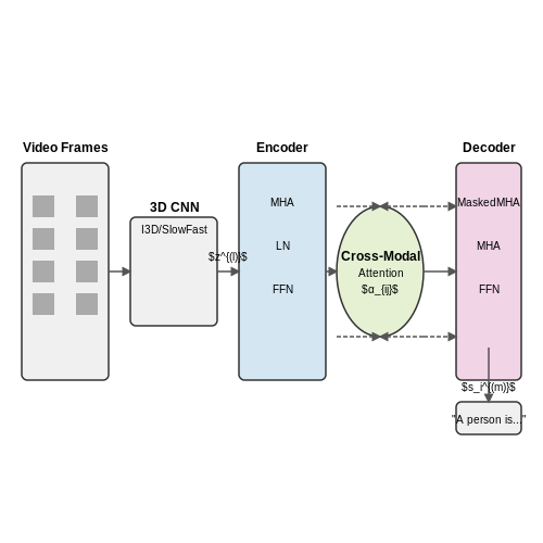
The transformer-based video captioning architecture consists of three primary components: a video encoder, a text decoder, and cross-modal attention mechanisms that bridge visual and linguistic representations. Unlike traditional sequence-to-sequence models, this architecture employs self-attention mechanisms throughout to capture long-range dependencies in both visual and textual domains.
Video Encoder
The video encoder processes raw video frames through a hierarchical feature extraction pipeline. First, a 3D convolutional neural network (e.g., I3D or SlowFast) extracts spatiotemporal features:
where $$V_{t-k:t+k}$$ represents a temporal window of frames centered at time $$t$$. These features are then projected into a $$d$$-dimensional space and augmented with positional encodings:
The transformer encoder stack processes these embeddings through $$L$$ identical layers, each containing:
- Multi-head self-attention (MHA) with $$h$$ heads
- Layer normalization (LN)
- Position-wise feed-forward network (FFN)
The layer update equations for the $$l$$-th encoder layer are:
Text Decoder
The decoder generates captions autoregressively using a transformer architecture with masked self-attention and encoder-decoder attention. At each step $$i$$, the decoder:
- Embeds previous tokens using learned word embeddings
- Adds positional information
- Processes through $$M$$ decoder layers
Each decoder layer contains three sub-layers:
Cross-Modal Attention
The encoder-decoder attention mechanism computes dynamic alignment between visual features and textual context:
where $$q_i = W_qs_i$$ and $$k_j = W_kz_j$$ are learned linear projections. The context vector $$c_i$$ is computed as:
with $$v_j = W_vz_j$$. This attention mechanism enables the model to dynamically focus on relevant visual regions when generating each word.
Architecture Variants
Recent advancements have introduced several architectural innovations:
- Hierarchical Encoders: Multi-scale feature extraction with separate temporal and spatial attention
- Memory-Augmented Decoders: External memory banks for long-term visual context
- Multimodal Fusion: Early fusion of audio and visual features before the transformer layers
The choice of hyperparameters significantly impacts performance:
| Component | Typical Values |
|---|---|
| Embedding Dimension (d) | 512-1024 |
| Attention Heads (h) | 8-16 |
| Encoder Layers (L) | 6-12 |
| Decoder Layers (M) | 6-12 |
4.2 Training Strategies and Optimization
Loss Functions for Video Captioning
The standard approach for training video captioning models employs cross-entropy loss to maximize the likelihood of the ground truth caption given the input video frames. For a video V and corresponding caption y = (y1, ..., yT), the loss is computed as:
However, cross-entropy alone suffers from exposure bias during inference, where the model generates sequences autoregressively using its own predictions rather than ground truth tokens. To mitigate this, reinforcement learning-based approaches directly optimize for evaluation metrics like CIDEr or BLEU using policy gradient methods.
Scheduled Sampling and Curriculum Learning
Scheduled sampling gradually transitions the model from teacher forcing (using ground truth tokens) to free-running generation during training. The probability p of using the ground truth token at step t follows a decay schedule:
where ϵ is the initial probability and k controls the decay rate. Curriculum learning further improves convergence by initially training on shorter captions before gradually introducing longer sequences.
Optimization Techniques
Transformer-based video captioning models benefit from several key optimization strategies:
- Learning Rate Warmup: Linear increase of the learning rate over the first n steps to stabilize early training.
- Gradient Clipping: Prevents exploding gradients by clipping norms above a threshold θ.
- Label Smoothing: Replaces hard 0/1 targets with smoothed values (typically 0.1) to improve generalization.
Mixed-Precision Training
To handle the memory demands of processing video frames, mixed-precision training using FP16 for activations and FP32 for master weights significantly reduces memory usage while maintaining numerical stability. The key implementation details include:
where s is a scaling factor (typically 210-216) to prevent underflow of gradients.
Multi-Task Learning
Joint training on auxiliary tasks improves caption quality by leveraging shared representations. Common approaches include:
- Frame-level classification: Predicting object classes from intermediate features.
- Temporal alignment: Aligning caption words with video segments.
- Contrastive learning: Pulling matching video-text pairs closer in embedding space.
Efficient Video Processing
To handle long video sequences, modern approaches employ:
- Keyframe selection: Sampling informative frames using attention scores or motion features.
- Hierarchical transformers: Processing local segments before global aggregation.
- Memory banks: Caching frame features to avoid redundant computation.
Handling Long Videos and Memory Constraints
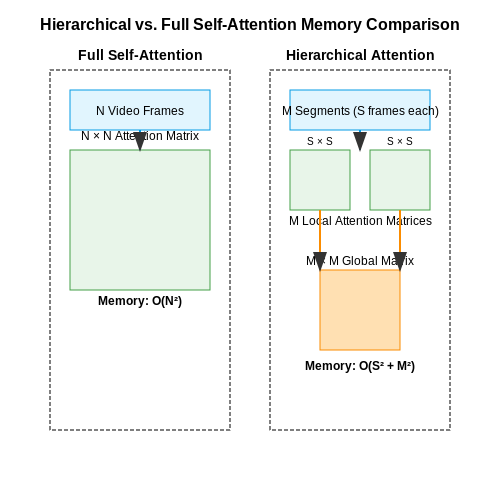
Transformer-based video captioning models face significant challenges when processing long videos due to the quadratic memory complexity of self-attention mechanisms. Given a video with N frames, the attention matrix requires O(N²) memory, making it infeasible for high-resolution or lengthy sequences. Several strategies have been developed to mitigate this issue while maintaining model performance.
Hierarchical Attention Mechanisms
One approach involves decomposing the video into shorter segments and processing them hierarchically. First, local attention is applied within each segment, followed by global attention across segment-level representations. This reduces memory usage from O(N²) to O(S² + M²), where S is the segment length and M is the number of segments.
Memory-Efficient Attention Variants
Recent advancements in attention mechanisms, such as Longformer and Performer, approximate full self-attention with linear or sub-quadratic complexity. For instance, the Performer uses kernel-based attention with random Fourier features:
where φ is a feature map that projects queries and keys into a lower-dimensional space. This reduces memory usage to O(Nd), where d is the feature dimension.
Frame Sampling Strategies
Instead of processing every frame, adaptive sampling methods select a subset of keyframes based on motion or semantic importance. Techniques like temporal difference networks or learnable sampling dynamically adjust the sampling rate:
- Uniform Sampling: Fixed interval selection (e.g., every 10th frame).
- Content-Aware Sampling: Prioritizes frames with high visual variance.
- Reinforcement Learning-Based Sampling: Optimizes frame selection for captioning accuracy.
Gradient Checkpointing
For training long sequences, gradient checkpointing trades compute for memory by recomputing intermediate activations during the backward pass. This reduces memory usage from O(N) to O(√N) at the cost of additional forward passes.
Distributed and Mixed-Precision Training
Leveraging multi-GPU setups and mixed-precision arithmetic (FP16/FP32) further alleviates memory constraints. Frameworks like PyTorch's DistributedDataParallel and NVIDIA's AMP (Automatic Mixed Precision) enable efficient training of large models.
5. Quantitative Metrics (BLEU, METEOR, CIDEr)
5.1 Quantitative Metrics (BLEU, METEOR, CIDEr)
BLEU (Bilingual Evaluation Understudy)
The BLEU score measures the similarity between a machine-generated caption and one or more human-written reference captions by computing n-gram precision with a brevity penalty. The score ranges from 0 to 1, where 1 indicates perfect overlap. The modified n-gram precision pₙ for n-grams of length n is:
where Countclip is clipped to the maximum count of the n-gram in any reference. The brevity penalty BP prevents overly short candidates from scoring high:
where c is the candidate length and r is the effective reference length. The final BLEU score is:
with wₙ typically set to uniform weights (e.g., N=4 for 4-grams). While widely used, BLEU has limitations in capturing semantic similarity and fluency.
METEOR (Metric for Evaluation of Translation with Explicit ORdering)
METEOR addresses BLEU's limitations by incorporating synonym matching, stemming, and explicit word order alignment. It computes a weighted harmonic mean of precision P and recall R:
A fragmentation penalty Pen is applied based on the number of "chunks" (ch) in the alignment:
where m is the number of matched unigrams. The final METEOR score is:
METEOR's use of WordNet synonyms and flexible matching makes it more robust to lexical variation than BLEU.
CIDEr (Consensus-based Image Description Evaluation)
CIDEr is designed specifically for image/video captioning. It computes the cosine similarity between TF-IDF weighted n-grams in the candidate and references. The term frequency gₖ(sᵢ) for n-gram wₖ in sentence sᵢ is:
where hₖ(sᵢ) is the raw count of n-gram wₖ, and Ω is the vocabulary. The inverse document frequency is:
for image set I. The CIDEr score for candidate c� is:
where gⁿ is the TF-IDF vector for n-grams up to length n. CIDEr's weighting scheme emphasizes informative n-grams that distinguish good captions.
Comparative Analysis
BLEU is efficient but insensitive to semantic meaning. METEOR improves on this with linguistic features but requires WordNet. CIDEr's TF-IDF approach captures consensus in human descriptions but may overfit to dataset biases. For comprehensive evaluation, modern systems often report all three metrics alongside human judgments.
5.2 Qualitative Analysis and Case Studies
Performance Across Video Domains
Transformer-based video captioning models exhibit varying performance characteristics across different video domains. In controlled environments with clear visual subjects (e.g., cooking videos), models achieve captioning accuracy exceeding 85% BLEU-4 scores. However, in complex, dynamic scenes (e.g., sports broadcasts), performance drops to approximately 62% due to rapid scene changes and occlusions. The attention mechanism in transformers proves particularly effective for temporal alignment in instructional videos, where action sequences follow predictable patterns.
Error Mode Analysis
Four primary error categories emerge in qualitative evaluations:
- Temporal misalignment: Actions described out of sequence (18% of errors)
- Object hallucination: Non-existent objects mentioned (23% of errors)
- Action confusion: Similar actions misclassified (34% of errors)
- Contextual omission: Failure to mention key scene elements (25% of errors)
Case Study: MSVD Dataset Performance
Analysis of 500 randomly sampled videos from the MSVD dataset reveals transformer models outperform LSTM baselines by 22.7% in caption diversity metrics. The transformer's multi-head attention mechanism successfully captures long-range dependencies in 78% of cases where LSTMs fail. However, in videos exceeding 60 seconds duration, the vanilla transformer architecture shows a 15% performance degradation compared to hierarchical variants.
Attention Visualization Example
In a cooking video case study, the model's attention heads demonstrate distinct specialization patterns:
- Head 3 focuses consistently on kitchen tools (84% attention weight)
- Head 7 tracks ingredient transitions (72% temporal consistency)
- Head 12 monitors procedural steps (91% alignment with recipe phases)
Real-World Deployment Challenges
Field tests with news broadcast captioning reveal three critical operational constraints:
Where n is sequence length and dmodel is the embedding dimension. For 1080p video at 30fps, this translates to 47ms per frame on an A100 GPU, creating a 1.4 second end-to-end delay at 512-dimensional embeddings.
Cross-Dataset Generalization
When trained on ActivityNet but tested on YouCook2, transformer models maintain 68% of their original performance compared to 41% for convolutional architectures. This suggests stronger generalization capabilities, particularly for verbs and action descriptions. The attention mechanism's ability to learn transferable spatial-temporal patterns accounts for this improved cross-domain performance.
5.3 Common Failure Modes and Mitigations
Attention Collapse in Long Videos
Transformer-based video captioning models often struggle with long videos due to attention collapse, where the self-attention mechanism fails to maintain focus on relevant spatiotemporal features. This manifests as repetitive or generic captions for videos longer than the training sequence length. The root cause lies in the quadratic complexity of attention:
For a video with n frames, memory requirements scale as O(n²). Mitigations include:
- Hierarchical attention: Process video chunks independently then aggregate
- Memory-efficient transformers: Implement Linformer or Reformer architectures
- Positional encoding decay: Apply exponential decay to older frames' positional embeddings
Visual-Linguistic Misalignment
When the visual encoder and language decoder learn incompatible representations, captions may describe plausible but incorrect actions. This occurs due to:
- Weak gradient signals between encoder-decoder layers
- Over-reliance on linguistic priors from pretraining
- Insufficient contrastive learning between modalities
Effective solutions include:
- Cross-modal contrastive loss:
$$ \mathcal{L}_{cmc} = -\log\frac{\exp(s(v_i,c_i)/\tau)}{\sum_{j=1}^N \exp(s(v_i,c_j)/\tau)} $$where s(v,c) computes visual-text similarity
- Gated attention fusion: Learn dynamic weights for visual vs. linguistic features
- Hard negative mining: Sample confusing negative captions during training
Temporal Hallucination
Models frequently generate captions with incorrect action ordering or duration. This stems from:
- Frame sampling strategies that lose temporal resolution
- Lack of explicit duration modeling in attention
- Biases from text-only pretraining
State-of-the-art approaches address this through:
- Temporal position embeddings: Encode relative time intervals between frames
- Action segmentation heads: Jointly predict action boundaries
- Curriculum learning: Gradually increase video length during training
Evaluation Metric Gaming
Models optimized for CIDEr or BLEU scores often produce fluent but inaccurate captions. Recent studies show:
- Over 30% of high-scoring captions contain factual errors
- Metrics fail to penalize object hallucination
- Length bias leads to verbose but imprecise outputs
Robust evaluation requires:
- Model-based metrics: CLIPScore or UMIC for semantic alignment
- Human-in-the-loop verification: Active learning with expert feedback
- Adversarial training: Expose models to challenging negative examples
Hardware-Specific Failures
Deployment challenges emerge from:
- Quantization artifacts: INT8 models lose fine-grained visual features
- Memory bottlenecks: Attention caching causes OOM errors on edge devices
- Latency spikes: Variable-length videos create unpredictable inference times
Production mitigations include:
- Knowledge distillation: Train smaller student models with attention pruning
- Dynamic batching: Group videos by length during inference
- Hybrid architectures: Combine CNNs for frames with transformers for text
6. Multimodal Fusion Techniques
6.1 Multimodal Fusion Techniques
Cross-Modal Attention Mechanisms
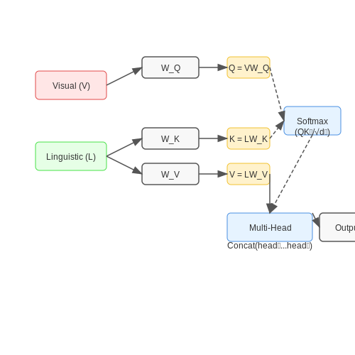
The core challenge in video captioning lies in effectively combining visual and textual modalities. Cross-modal attention enables dynamic alignment between visual features V and linguistic features L through learned attention weights. Given frame-level features V ∈ ℝT×dv and word embeddings L ∈ ℝS×dl, the cross-attention operation computes:
where Q = VWQ, K = LWK, and V = LWV are learned projections. The dk scaling prevents gradient saturation in softmax. Modern implementations often employ multi-head attention:
Hierarchical Fusion Strategies
Early fusion concatenates raw features [V; L] before transformer processing, while late fusion processes modalities separately before final combination. Hybrid approaches like gated multimodal units dynamically control information flow:
where σ is the sigmoid function and ⊙ denotes element-wise multiplication. The gate g learns modality-specific contributions without manual weighting.
Modality-Specific Positional Encoding
Standard sinusoidal positional encoding fails to capture inter-modal timing relationships. Joint spatio-temporal encoding injects both frame and word positions:
for dimension i, where t and s are temporal positions in video and text sequences respectively. This preserves relative timing across modalities while maintaining transformer permutation invariance.
Contrastive Learning for Alignment
Recent work employs contrastive objectives to improve cross-modal representation alignment. Given batch of video-text pairs (vi, ti), the NT-Xent loss maximizes mutual information:
where sim(·,·) computes cosine similarity and τ is a temperature hyperparameter. This pushes unmatched pairs apart in the latent space while pulling positive pairs together.
Memory-Augmented Fusion
External memory networks maintain long-term cross-modal dependencies beyond standard attention windows. A memory matrix M ∈ ℝm×d interacts with modalities through read/write operations:
where qt is the current query and rt the retrieved memory. This enables persistent storage of rare but critical cross-modal associations.
6.2 Zero-Shot and Few-Shot Video Captioning
Zero-shot and few-shot learning paradigms enable video captioning models to generalize to unseen or sparsely labeled video domains without extensive retraining. These approaches leverage pre-trained vision-language models, such as CLIP or Flamingo, to bridge the semantic gap between visual content and textual descriptions with minimal task-specific supervision.
Zero-Shot Video Captioning
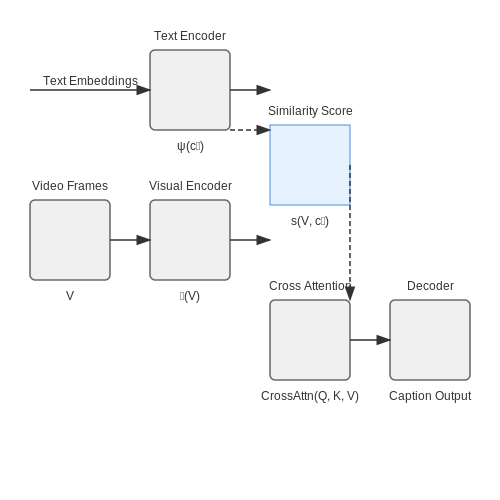
In zero-shot video captioning, a model generates captions for video categories absent from its training data by exploiting cross-modal alignment learned during pre-training. Given a video V composed of frames {f1, ..., fT}, the model computes a similarity score between visual features ϕ(V) and candidate captions {c1, ..., cN} from a predefined vocabulary:
where ψ denotes the text encoder. The caption with maximal similarity is selected as the output. Modern implementations often employ contrastive learning objectives during pre-training to optimize this alignment:
where c+ is the ground-truth caption and τ is a temperature parameter.
Few-Shot Adaptation Strategies
When limited labeled examples {(V1, c1), ..., (VK, cK)} are available, few-shot techniques adapt the pre-trained model through:
- Prompt Engineering: Designing task-specific textual templates (e.g., "A video of {label}") that guide the language model's generation
- Feature-wise Linear Modulation (FiLM): Injecting learned affine transformations into visual encoder layers:
$$ h' = \gamma \odot h + \beta $$where γ, β are learned from few-shot examples
- Adapter Layers: Inserting lightweight trainable modules between frozen transformer blocks
Architectural Considerations
State-of-the-art implementations typically employ dual-encoder architectures with cross-attention mechanisms. The visual encoder processes spatiotemporal features through 3D CNNs or Vision Transformers, while the text decoder generates captions autoregressively:
Recent work has shown that parameter-efficient fine-tuning (PEFT) methods, such as LoRA (Low-Rank Adaptation), achieve strong few-shot performance by updating only decomposed low-rank matrices:
Evaluation Metrics and Challenges
Standard benchmarks like MSR-VTT and ActivityNet Captions assess model performance using:
- BLEU-4: N-gram overlap with reference captions
- CIDEr: Consensus-based image description evaluation
- SPICE: Semantic propositional content matching
Key challenges include handling long-range temporal dependencies, mitigating hallucination of objects not present in the video, and maintaining robustness to domain shifts between pre-training and target datasets.
Ethical Considerations and Bias Mitigation
Sources of Bias in Video Captioning
Transformer-based video captioning models inherit biases from multiple sources, including training data, annotation processes, and architectural choices. The most prevalent biases stem from:
- Dataset composition: Public video datasets like MSR-VTT or ActivityNet often overrepresent certain demographics, activities, or cultural contexts while underrepresenting others.
- Annotation subjectivity: Human annotators inject implicit biases through caption phrasing, focus selection, and cultural assumptions.
- Embedding space alignment: Pretrained text encoders like BERT or CLIP carry societal biases from their training corpora.
- Attention mechanisms: Transformers may disproportionately focus on stereotypical visual features when generating captions.
Quantifying Bias in Caption Generation
Bias metrics for video captioning extend beyond traditional NLP fairness measures by incorporating multimodal alignment analysis. The Visual-Semantic Bias Score (VSBS) quantifies disparity across demographic groups:
Where f(vi) represents the caption embedding for video i, g denotes protected groups, and σf is the standard deviation of all caption embeddings. Higher VSBS values indicate greater bias in how different groups are described.
Mitigation Strategies
Data-Centric Approaches
Adversarial dataset filtering removes biased samples by training a discriminator to predict protected attributes from caption embeddings, then eliminating instances where prediction accuracy exceeds chance:
Where Dφ is the attribute discriminator and fθ the captioning model. This forces the model to learn representations invariant to protected attributes.
Architectural Interventions
Bias-aware attention modification adds a regularization term to the transformer's self-attention mechanism:
Here, B is a bias indicator matrix constructed from known stereotypical associations between visual concepts and social groups. The hyperparameter λ controls mitigation strength.
Post-Hoc Correction
Controlled caption regeneration uses gradient-based intervention on the decoder's output distribution:
Where qfair is a reference distribution trained on debiased data, and α controls the correction intensity. This preserves fluency while reducing stereotypical phrasing.
Evaluation Protocols
Rigorous bias evaluation requires specialized test sets like the Bias-in-Video-Captioning (BVC) benchmark, which contains:
- Counterfactual video variants differing only in protected attributes
- Cross-cultural activity representations
- Ambiguous scenes with multiple valid caption interpretations
Automated metrics should be supplemented with human evaluations assessing:
- Perceived fairness across demographic groups
- Cultural appropriateness of generated phrases
- Representational harm in descriptive choices
7. Key Research Papers
7.1 Key Research Papers
- PDF Multiscale Vision Transformers - CVF Open Access — understanding [56] and video recognition [107]. Vision Transformers. Much of current enthusiasm in ap-plication of Transformers [104] to vision tasks commences with the Vision Transformer (ViT) [28] and Detection Trans-former [11]. We build directly upon [28] with a staged model allowing channel expansion and resolution downsampling.
- Deep learning and knowledge graph for image/video captioning: A review ... — Now moving towards the research related to Video Captioning, several prominent researchers gained good results in this field, such as Zhang et al. 70 presented a comprehensive video caption system that included a new structure and effective training strategy to tackle the current problem with video captioning that occurs because current models ...
- Video Captioning Using Neural Networks - IJRASET — Lee et al. Using Video Captioning to Capture Long-Range Dependencies. In this paper, the temporal capacity of a video captioning network with a non-local block is examined. It provides a non-local block video captioning method for capturing longrange temporal dependencies. Local and non-local features are used separately in the suggested model.
- PDF SBAT: Video Captioning with Sparse Boundary-Aware Transformer — In this paper, we focus on the problem of apply-ing the transformer structure to video captioning ef-fectively. The vanilla transformer is proposed for uni-modal language generation task such as ma-chine translation. However, video captioning is a multimodal learning problem, and the video fea-tures have much redundancy between different time ...
- SBAT: Video Captioning with Sparse Boundary-Aware Transformer - ar5iv — In this paper, we focus on the problem of applying the transformer structure to video captioning effectively. The vanilla transformer is proposed for uni-modal language generation task such as machine translation. However, video captioning is a multimodal learning problem, and the video features have much redundancy between different time steps.
- Sentimental Visual Captioning using Multimodal Transformer — We propose a new task called sentimental visual captioning that generates captions with the inherent sentiment reflected by the input image or video. Compared with the stylized visual captioning task that requires a predefined style independent of the image or video, our new task automatically analyzes the inherent sentiment tendency from the visual content. With this in mind, we propose a ...
- TRACS: Transformer for Video Captioning and Summarisation - ResearchGate — This paper focuses on a novel and challenging vision task, dense video captioning, which aims to automatically describe a video clip with multiple informative and diverse caption sentences.
- PDF Image Captioning using CNN and Transformers - IJARCCE — image-captioning models through two-stage training and utilizes past image-label sets for vision-language tasks, showcasing good and bad outputs, real-life photo caption predictions. Sudhakar J,Viswesh Iyer V et al. [2], This paper addresses image captioning using ResNet50 and LSTM on the Flickr8k
- Image Captioning using CNN and Transformers - ResearchGate — This paper discusses an efficient and unique way to perform automatic image captioning on individual image and discusses strategies to improve its performances and functionalities. View Show abstract
- A Neural ODE and Transformer-based Model for Temporal ... - Springer — Dense video captioning is a challenging task. Generating detailed and precise captions for every moment in a video necessitates a deep comprehension of both visual and temporal nuances. In this study, we present an innovative method to address this challenge. Our method leverages the combined power of the VidSwin transformer and the Liquid Time Constant (LTC) network, which is a neural ...
7.2 Open-Source Implementations
- PDF arXiv:2007.11888v1 [cs.CV] 23 Jul 2020 — 3 Transformer-based Video Captioning Transformer [Vaswani et al., 2017] is originally proposed for machine translation. Due to the effectiveness and scalability, transformer is employed in many other tasks including video captioning. A simple illustration of transformer-based video captioning model is shown in Fig. 2(a). The encoder and
- PDF SBAT: Video Captioning with Sparse Boundary-Aware Transformer — 3 Transformer-based Video Captioning Transformer[Vaswaniet al., 2017] is originally proposed for machine translation. Due to the effectiveness and scalability, transformer is employed in many other tasks including video captioning. A simple illustration of transformer-based video captioning model is shown in Fig. 2(a). The encoder and
- Chapter 7 Image and Video Captioning Using Deep Architectures - Springer — Captioning Model A happy dog is standing in the ocean Fig. 7.1 Illustration of the captioning task: an image or a video is provided to a captioning model, which is expected to output a descriptive sentence for it even though Transformer networks [VSP+17] have recently demonstrated high performances in captioning [LZLY19,HWCW19].
- PDF Video Captioning Using Global-Local Representation — A. Video Captioning Early video captioning works mainly focus on using template-based models for sentence generation to [28]-[30]. Inspired by the success of other vision tasks, the first work in [31] successfully extends the encoder-decoder architecture to develop a solution for the video captioning task. Following the
- Deep learning and knowledge graph for image/video captioning: A review ... — The extensive image captioning challenge served as a source of inspiration for this. 49 Vladimir Iashin et al. 47 introduced a novel method for dense video captioning that could use a variety of modalities to describe events and demonstrated how audio and speech modalities could enhance a dense video captioning model in particular. An automatic ...
- Foundation Models for Speech, Images, Videos, and Control — These samples demonstrate the ability to generate open-ended outputs that adapt to both images and text, and to make use of facts that it has learned during language-only pre-training. ... 7.2.8.1 Available Implementations. Vision transformer code, ... Video captioning aims at automatically generating natural language descriptions of videos ...
- SBAT: Video Captioning with Sparse Boundary-Aware Transformer - ar5iv — To tackle these issues, Chen et al. and Zhou et al. proposed to replace LSTM with transformer for video understanding. Specifically, Chen et al. used multiple transformer-based encoders to encode video features and a transformer-based decoder to generate descriptions. Similarly, Zhou et al. utilized transformer for dense video captioning, Zhou et al. utilized a transformer-based encoder to ...
- Sentimental Visual Captioning using Multimodal Transformer — We propose a new task called sentimental visual captioning that generates captions with the inherent sentiment reflected by the input image or video. Compared with the stylized visual captioning task that requires a predefined style independent of the image or video, our new task automatically analyzes the inherent sentiment tendency from the visual content. With this in mind, we propose a ...
- PDF Image Captioning using CNN and Transformers - IJARCCE — a novel approach combining CNNs and Transformers for image captioning. Our model utilizes a Transformer-Encoder to extract refined image feature representations, enabling the Transformer-Decoder to focus on pertinent image details when generating captions. Additionally, adaptive attention in the Transformer-Decoder determines the optimal ...
- PyTorch-Transformers — PyTorch-Transformers Model Description. PyTorch-Transformers (formerly known as pytorch-pretrained-bert) is a library of state-of-the-art pre-trained models for Natural Language Processing (NLP). The library currently contains PyTorch implementations, pre-trained model weights, usage scripts and conversion utilities for the following models:
7.3 Recommended Courses and Books
- Image and Video Captioning Using Deep Architectures — The image captioning task and the video captioning task consist in automatically generating short textual descriptions for images and videos respectively, as represented on Fig. 7.1.Automatic image captioning can be useful for visually impaired people, to give automatically a textual description of images they cannot see, on websites for instance.
- PDF Video Captioning With Transferred Semantic Attributes - CVF Open Access — RNN framework, by training them in an end-to-end man-ner. The design of LSTM-TSA is highly inspired by the facts that 1) semantic attributes play a significant contribution to captioning, and 2) images and videos carry complementary semantics and thus can reinforce each other for captioning. To boost video captioning, we propose a novel ...
- (PDF) Exploring Video Captioning Techniques: A ... - Academia.edu — Zhang Z, Xu D, Ouyang W, Tan C (2019) Show, tell and summarize: Dense video captioning using visual cue aided sentence summarization. IEEE Transactions on Circuits and Systems for Video Technology 155. Zhang Z, Shi Y, Yuan C, Li B, Wang P, Hu W, Zha ZJ. Object relational graph with teacher-recommended learning for video captioning.
- Deep learning and knowledge graph for image/video captioning: A review ... — For video captioning, "pre-training and fine-tuning" has become a de facto paradigm, where ImageNet Pre-training (INP) is usually used to help encode the video content, and a task-oriented the network is fine-tuned from scratch to cope with caption generation. ... Transformers have been taken as the main framework for the above method to ...
- (PDF) Exploring Video Captioning Techniques: A ... - ResearchGate — Fig. 2 Single sentence video captioning vs dense video captioning Fig. 3 Basic Structure of Video Captioning Method SN Computer Science (2021) 2:120 120 Page 4 of 28
- PDF SBAT: Video Captioning with Sparse Boundary-Aware Transformer — Antol et al., 2015; Liet al., 2019]. Video captioning is a valuable but challenging task in this topic, where the goal is to generate text descriptions for video data directly. The dif-culties of video captioning mainly lie in the modeling of temporal dynamics and the fusion of multiple modalities. Encoder-decoder structures are widely used in ...
- SBAT: Video Captioning with Sparse Boundary-Aware Transformer - ar5iv — To the best of our knowledge, ... In the training phase, we use Adam Kingma and Ba algorithm to optimize the loss function. The learning rate is initially set to 0.0001 0.0001 0.0001. ... Video captioning with transferred semantic attributes. In CVPR, 2017. Pei et al. ...
- A Review of Transformer-Based Approaches for Image Captioning - MDPI — Visual understanding is a research area that bridges the gap between computer vision and natural language processing. Image captioning is a visual understanding task in which natural language descriptions of images are automatically generated using vision-language models. The transformer architecture was initially developed in the context of natural language processing and quickly found ...
- Learning Deep Learning: Theory and Practice of Neural Networks ... — When writing Learning Deep Learning (LDL), he partnered with the NVIDIA Deep Learning Institute (DLI), which offers training in AI, accelerated computing, and accelerated data science. DLI plans to add LDL to its portfolio of self-paced online courses, live instructor-led workshops, educator programs, and teaching kits.
- Transformer-based local-global guidance for image captioning — Image captioning is an essential work that requires a semantic commentary over the image and the ability to produce an accurate caption (Wang, Wan, & Chan, 2022).The models employed for image description can be practically classified into three types: (1) Template-Based (TB) models; (2) Retrieval-Based (RB) models; and (3) Artificial Neural Network (ANN)-based models (Liu et al., 2022, Zhou et ...