Modulation Techniques
1. Definition and Purpose of Modulation
1.1 Definition and Purpose of Modulation
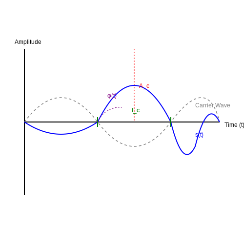
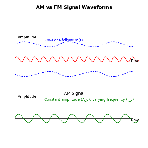
Modulation is the systematic alteration of a carrier signal—typically a high-frequency sinusoidal wave—by an information-bearing signal (baseband signal). This process enables the efficient transmission of data over communication channels by shifting the spectral content of the baseband signal to a frequency range suitable for propagation. The mathematical representation of a carrier wave is:
where Ac is the amplitude, fc the carrier frequency, and ϕc the phase. Modulation modifies one or more of these parameters proportionally to the baseband signal m(t).
Fundamental Objectives
- Frequency Translation: Baseband signals (e.g., audio at 20 Hz–20 kHz) are unsuited for long-distance transmission due to attenuation and antenna size constraints. Modulation upconverts the signal to RF/Microwave bands (e.g., 88–108 MHz for FM radio).
- Multiplexing: Enables simultaneous transmission of multiple signals via frequency-division (FDM) or quadrature carriers (QAM).
- Noise Immunity: Certain modulation schemes (e.g., FM, PSK) exhibit superior resilience to channel impairments compared to baseband transmission.
Key Mathematical Formulations
For amplitude modulation (AM), the modulated signal becomes:
where ka is the amplitude sensitivity. For angle modulation (FM/PM), the instantaneous phase deviates proportionally to m(t):
Practical Applications
In 5G NR, orthogonal frequency-division multiplexing (OFDM) combines QAM with multi-carrier modulation to achieve spectral efficiencies >30 bps/Hz. Satellite communications rely on phase-shift keying (PSK) for its power efficiency in low-SNR environments.
1.2 Key Components: Carrier and Modulating Signals
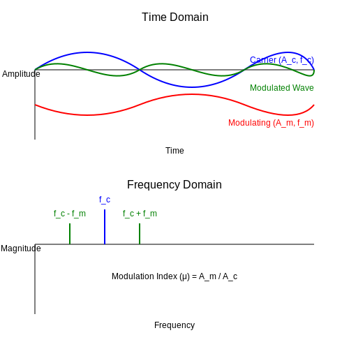
Modulation fundamentally involves two signals: the carrier signal and the modulating signal. The carrier is typically a high-frequency sinusoidal wave, while the modulating signal contains the information to be transmitted. Their interaction forms the basis of all modulation techniques.
Mathematical Representation
A carrier wave can be expressed as:
where:
- Ac is the carrier amplitude
- fc is the carrier frequency
- ϕc is the carrier phase
The modulating signal, representing the information, is generally a baseband signal:
Modulation Process
During modulation, one or more parameters of the carrier (amplitude, frequency, or phase) are varied in proportion to the modulating signal. For amplitude modulation (AM), the resulting signal becomes:
This equation shows the carrier envelope being shaped by the modulating signal. The modulation index μ quantifies the extent of modulation:
Spectral Characteristics
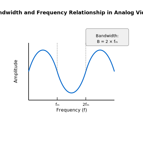
Modulation creates sidebands around the carrier frequency. For a sinusoidal modulating signal, AM produces two sidebands at fc ± fm. The bandwidth required is twice the highest frequency component of the modulating signal.
Practical Considerations
In real systems, carrier signals are generated by stable oscillators (e.g., crystal or SAW oscillators for RF applications), while modulating signals often undergo preprocessing (filtering, compression) before modulation. The choice between carrier frequencies involves tradeoffs between propagation characteristics, antenna size, and available spectrum.
Modern systems frequently use complex carriers, such as:
- Orthogonal frequency-division multiplexing (OFDM) carriers
- Spread spectrum signals
- Ultra-wideband pulses
Digital modulation extends these concepts by representing information as discrete symbols that modify the carrier's parameters. The modulating signal becomes a sequence of symbols, with each symbol representing multiple bits through constellation mapping.
1.3 Bandwidth and Spectral Efficiency
Fundamental Relationship Between Bandwidth and Data Rate
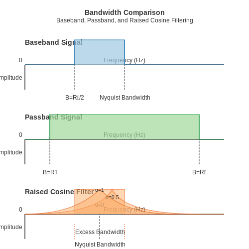
The bandwidth B of a modulated signal is directly tied to the symbol rate Rs and the modulation order M. For a baseband system using Nyquist pulse shaping, the minimum required bandwidth is:
where Rs is the symbol rate in baud. When using passband modulation (e.g., QAM, PSK), the required bandwidth doubles due to the positive and negative frequency components:
The spectral efficiency η, measured in bits per second per Hertz (bps/Hz), quantifies how efficiently a modulation scheme utilizes bandwidth:
where Rb is the bit rate. For an M-ary modulation scheme with k = log2M bits per symbol, the maximum theoretical spectral efficiency becomes:
Practical Limitations and Trade-offs
Real-world systems rarely achieve the theoretical maximum spectral efficiency due to:
- Channel impairments: Multipath fading, noise, and interference necessitate error-correction coding, reducing effective η.
- Filter roll-off: Practical pulse-shaping filters (e.g., raised cosine) require excess bandwidth characterized by the roll-off factor α:
For example, LTE systems typically use α = 0.22, meaning 22% more bandwidth than the Nyquist minimum.
Comparative Analysis of Modulation Schemes
The table below shows spectral efficiencies for common digital modulation techniques:
| Modulation | Bits/Symbol (k) | Theoretical η (bps/Hz) | Practical η (with coding) |
|---|---|---|---|
| BPSK | 1 | 1 | 0.5–0.8 |
| QPSK | 2 | 2 | 1.4–1.6 |
| 16-QAM | 4 | 4 | 3.0–3.5 |
| 64-QAM | 6 | 6 | 4.5–5.0 |
Advanced Techniques for Spectral Efficiency
Modern systems employ several methods to push beyond traditional limits:
- OFDM (Orthogonal Frequency Division Multiplexing): Divides bandwidth into orthogonal subcarriers, enabling dense packing. Used in 802.11ax (Wi-Fi 6) with η up to 9.6 bps/Hz.
- MIMO (Multiple-Input Multiple-Output): Spatial multiplexing increases capacity linearly with the number of antennas. 4×4 MIMO can quadruple η under ideal conditions.
- Non-Orthogonal Multiple Access (NOMA): Overlaps users in power domain, achieving higher multiplexing gains than OFDMA.
where C is the channel capacity, S/N is the signal-to-noise ratio. This establishes the absolute limit for spectral efficiency in additive white Gaussian noise (AWGN) channels.
Case Study: 5G NR Spectral Efficiency
5G New Radio (NR) achieves peak η of 30 bps/Hz through:
- 256-QAM modulation (8 bits/symbol)
- 8×8 MIMO spatial layers
- Flexible numerology with subcarrier spacing adaptation
The actual deployed efficiency ranges from 3–15 bps/Hz depending on channel conditions and beamforming gains.
2. Amplitude Modulation (AM)
2.1 Amplitude Modulation (AM)
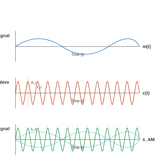
Amplitude Modulation (AM) is a linear modulation technique where the amplitude of a high-frequency carrier wave is varied in proportion to the instantaneous amplitude of the modulating signal. The mathematical representation of an AM signal is derived as follows:
where:
- \( s(t) \) is the modulated signal,
- \( A_c \) is the amplitude of the carrier wave,
- \( k_a \) is the amplitude sensitivity of the modulator,
- \( m(t) \) is the baseband message signal,
- \( f_c \) is the carrier frequency.
Modulation Index and Overmodulation
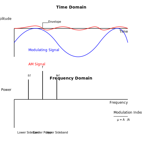
The modulation index (\( \mu \)) quantifies the extent of amplitude variation and is defined as:
For distortion-free transmission, \( \mu \) must satisfy \( 0 \leq \mu \leq 1 \). Overmodulation (\( \mu > 1 \)) leads to envelope distortion, requiring synchronous detection for recovery.
Frequency Domain Analysis
Fourier transforming the AM signal reveals its spectral composition:
where \( M(f) \) is the Fourier transform of \( m(t) \). The spectrum consists of:
- A carrier component at \( \pm f_c \),
- Upper and lower sidebands containing the message signal's spectral content.
Power Distribution and Efficiency
The total power \( P_t \) of an AM signal is distributed between the carrier and sidebands:
where \( P_c = A_c^2/2 \) is the carrier power. The sidebands carry only \( \frac{\mu^2}{2 + \mu^2} \times 100\% \) of the total power, leading to a maximum efficiency of 33.3% for \( \mu = 1 \).
Practical Applications
AM is widely used in:
- Broadcast radio (530–1700 kHz AM band), where its simple receiver design enables cost-effective mass communication.
- Aircraft communication systems, utilizing DSB-AM for voice transmission in the VHF band.
- QAM schemes, where AM is combined with phase modulation for higher spectral efficiency.
Demodulation Techniques
Common AM demodulation methods include:
- Envelope detection using diode rectifiers, effective only for \( \mu \leq 1 \).
- Synchronous detection requiring a phase-coherent local oscillator.
- Square-law detection exploiting nonlinear device characteristics.
2.2 Frequency Modulation (FM)
Fundamentals of Frequency Modulation
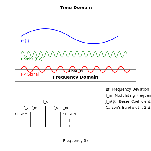
Frequency Modulation (FM) is a nonlinear modulation technique where the instantaneous frequency of the carrier signal varies in proportion to the amplitude of the modulating signal. Unlike Amplitude Modulation (AM), FM encodes information in the frequency domain, making it more resilient to amplitude-based noise and interference.
The general form of an FM signal is given by:
where:
- Ac is the carrier amplitude,
- fc is the carrier frequency,
- kf is the frequency sensitivity (Hz/volt),
- m(t) is the modulating signal.
Frequency Deviation and Modulation Index
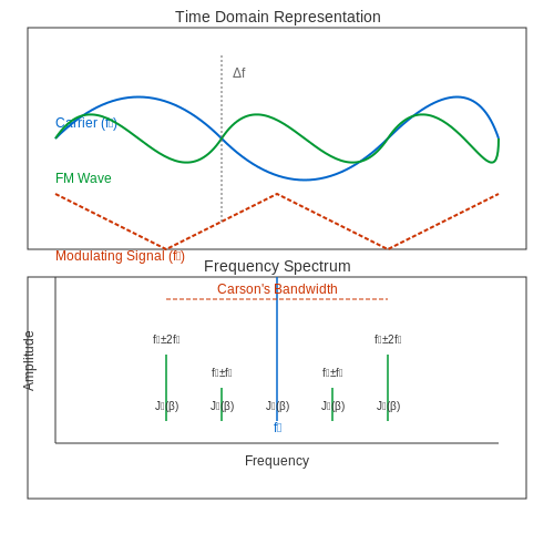
The peak frequency deviation (Δf) represents the maximum shift from the carrier frequency and is directly proportional to the amplitude of the modulating signal:
The modulation index (β) quantifies the extent of frequency modulation relative to the modulating signal's bandwidth (B):
For sinusoidal modulation with m(t) = Amcos(2πfmt), the modulation index simplifies to:
Spectrum of FM Signals
The frequency spectrum of an FM signal contains the carrier frequency and an infinite number of sidebands spaced at integer multiples of the modulating frequency. The amplitudes of these components are determined by Bessel functions of the first kind (Jn(β)):
For practical purposes, the bandwidth can be approximated using Carson's rule:
Narrowband vs. Wideband FM
FM systems are classified based on the modulation index:
- Narrowband FM (NBFM): β ≪ 1, bandwidth ≈ 2fm (similar to AM)
- Wideband FM (WBFM): β > 1, bandwidth follows Carson's rule
WBFM provides better noise immunity at the expense of bandwidth, making it suitable for high-fidelity audio broadcasting (e.g., FM radio with β ≈ 5).
Practical Implementation
FM generation typically employs voltage-controlled oscillators (VCOs) or phase-locked loops (PLLs). Demodulation can be achieved through:
- Slope detectors (using tuned circuits)
- Phase-locked loop demodulators
- Foster-Seeley discriminators
- Quadrature detectors
Applications and Advantages
FM is widely used in:
- Commercial radio broadcasting (88-108 MHz)
- Television audio transmission
- Two-way radio communications
- Microwave relay systems
Key advantages over AM include:
- Superior noise and interference rejection
- Constant envelope enables efficient RF power amplification
- Better adjacent channel interference performance
Limitations and Trade-offs
The improved performance comes with:
- Larger bandwidth requirements
- More complex transmitter and receiver designs
- Nonlinear behavior requiring linear frequency response in components
2.3 Phase Modulation (PM)
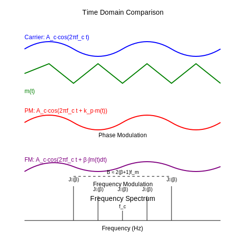
Phase modulation (PM) encodes information by varying the instantaneous phase of a carrier wave in proportion to the modulating signal. Unlike frequency modulation (FM), where the frequency deviation is the primary parameter, PM directly manipulates the phase angle of the carrier. The general form of a phase-modulated signal is:
where Ac is the carrier amplitude, fc is the carrier frequency, kp is the phase sensitivity (in radians per volt), and m(t) is the modulating signal. The instantaneous phase deviation is given by:
Relationship Between PM and FM
Phase modulation and frequency modulation are closely related. The instantaneous frequency deviation in PM is the time derivative of the phase deviation:
This means PM can be viewed as FM where the modulating signal is pre-emphasized by differentiation. Conversely, integrating the modulating signal before applying FM yields an equivalent PM signal.
Spectrum and Bandwidth
The spectrum of a phase-modulated signal is non-linear and depends on the modulation index β, defined as:
For a sinusoidal modulating signal m(t) = A_m \cos(2\pi f_m t), the PM signal can be expressed using Bessel functions:
where Jn(β) is the Bessel function of the first kind of order n. The bandwidth can be approximated using Carson's rule:
Practical Applications
Phase modulation is widely used in digital communication systems, such as:
- Quadrature Phase Shift Keying (QPSK) and higher-order PSK schemes, where discrete phase shifts encode digital symbols.
- Satellite communications, due to its resilience to noise and efficient bandwidth utilization.
- Optical fiber communications, where phase-modulated signals minimize nonlinear distortions.
Phase Modulation vs. Frequency Modulation
While PM and FM are mathematically related, they exhibit distinct practical differences:
- Noise performance: FM typically offers better noise immunity in analog systems due to inherent amplitude limiting.
- Implementation complexity: PM is often simpler to generate digitally, making it preferable in software-defined radio (SDR) systems.
- Spectral efficiency: PM can achieve higher data rates in digital systems through multi-level phase encoding.
Phase-Locked Loops in PM Demodulation
Phase-locked loops (PLLs) are commonly used for PM demodulation. The PLL tracks the instantaneous phase of the incoming signal, producing an output voltage proportional to the phase deviation. The transfer function of a PLL-based PM demodulator is:
where KVCO is the voltage-controlled oscillator gain and Kd is the phase detector gain.
Nonlinear Effects in PM
Phase modulation introduces nonlinear distortions when the modulation index exceeds certain limits. For large β, intermodulation products become significant, leading to spectral regrowth. This effect is particularly critical in:
- High-power amplifiers (HPAs), where AM/PM conversion can degrade signal integrity.
- Multi-carrier systems, where cross-phase modulation (XPM) induces crosstalk between channels.
3. Amplitude Shift Keying (ASK)
3.1 Amplitude Shift Keying (ASK)
Fundamental Concept
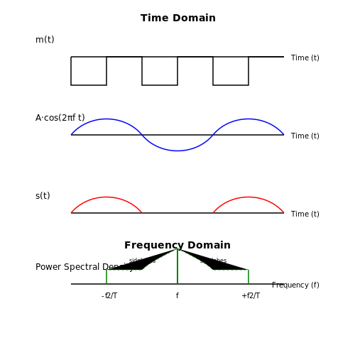
Amplitude Shift Keying (ASK) is a digital modulation technique where the amplitude of a carrier signal is varied in discrete steps to represent binary data. The simplest form, Binary ASK (BASK), uses two amplitude levels: one for logic 1 (typically the carrier’s full amplitude) and another for logic 0 (often zero amplitude). The modulated signal can be represented mathematically as:
where Ac is the carrier amplitude, fc is the carrier frequency, and m(t) is the binary message signal (0 or 1).
Modulation and Demodulation
ASK modulation is achieved by multiplying the carrier signal with the binary message. For coherent demodulation, a synchronous detector (e.g., a product detector) is used, requiring phase synchronization with the carrier. Non-coherent demodulation employs envelope detection, simplifying receiver design but sacrificing noise performance.
The power spectral density (PSD) of BASK is derived from its autocorrelation function:
where Tb is the bit duration. The PSD reveals a main lobe bandwidth of 2/Tb, with sidelobes decaying at a rate proportional to 1/f2.
Performance Analysis
The bit error rate (BER) for coherent ASK in additive white Gaussian noise (AWGN) is:
where Eb is the energy per bit, N0 is the noise power spectral density, and Q(·) is the Q-function. For non-coherent detection, the BER degrades to:
Practical Considerations
ASK is susceptible to amplitude noise and fading due to its reliance on amplitude variations. It finds use in low-cost applications like optical communications (e.g., infrared remote controls) and RFID systems, where simplicity outweighs spectral inefficiency. Variants like On-Off Keying (OOK) are a subset of ASK with zero amplitude for 0.
Comparison with Other Techniques
Unlike Frequency Shift Keying (FSK) or Phase Shift Keying (PSK), ASK’s spectral efficiency is lower due to its wider main lobe and sidelobes. However, its transmitter and receiver designs are simpler, making it suitable for power-constrained systems.
Frequency Shift Keying (FSK)
Frequency Shift Keying (FSK) is a digital modulation scheme where the carrier frequency is shifted between discrete values to represent binary data. Unlike amplitude-shift keying (ASK), FSK is less susceptible to noise since information is encoded in frequency variations rather than amplitude. The two most common variants are Binary FSK (BFSK), which uses two frequencies, and M-ary FSK (MFSK), which employs multiple frequencies for higher spectral efficiency.
Mathematical Representation
The modulated signal in BFSK can be expressed as:
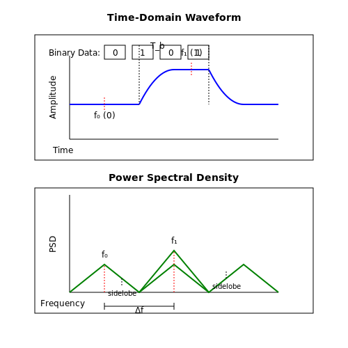
where A is the amplitude, f0 and f1 are the frequencies representing binary 0 and 1, and ϕi is the phase. The frequency separation Δf = |f1 − f0| must be chosen to ensure orthogonality, typically satisfying:
where Tb is the bit duration. For coherent detection, n = 1 minimizes bandwidth, while non-coherent detection requires n ≥ 2.
Power Spectral Density
The power spectral density (PSD) of BFSK with continuous phase (CPFSK) is derived from the autocorrelation function. For a rectangular pulse shape, the PSD is:
Discontinuous-phase FSK exhibits sidelobes due to abrupt frequency transitions, whereas CPFSK suppresses them, reducing adjacent-channel interference.
Modulation and Demodulation
FSK generation can be achieved via:
- Voltage-controlled oscillators (VCOs): Directly modulate the input data to vary the oscillator frequency.
- Phase-locked loops (PLLs): Switch between synchronized frequency sources.
Demodulation techniques include:
- Coherent detection: Uses matched filters or correlators for optimal performance but requires carrier recovery.
- Non-coherent detection: Employs envelope detectors or frequency discriminators, trading robustness for simplicity.
Performance in Noise
The bit error rate (BER) for coherent BFSK in additive white Gaussian noise (AWGN) is:
where Eb is the energy per bit, N0 is the noise spectral density, and Q(·) is the Q-function. Non-coherent detection incurs a ~3 dB penalty:
Applications
FSK is widely used in:
- Telemetry systems: Due to its noise resilience in low-power scenarios (e.g., satellite communications).
- RFID and NFC: Where simple demodulation suits passive tags.
- Modems (e.g., V.21, V.23): For early dial-up networks.
Phase Shift Keying (PSK)
Phase Shift Keying (PSK) is a digital modulation scheme where the phase of the carrier signal is varied in accordance with the modulating data signal. Unlike amplitude or frequency modulation, PSK encodes information in the instantaneous phase of the carrier, making it highly efficient in bandwidth utilization and noise resilience.
Mathematical Representation of PSK
The general form of a PSK-modulated signal is given by:
where:
- A is the amplitude of the carrier,
- fc is the carrier frequency,
- φi(t) represents the phase shift corresponding to the symbol being transmitted.
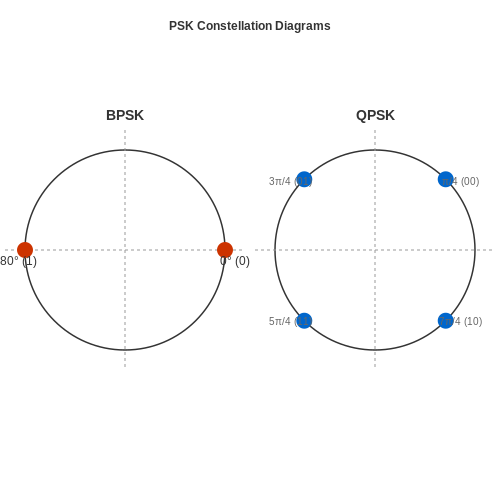
For binary PSK (BPSK), the phase takes two values (0° and 180°), representing binary 0 and 1:
M-ary PSK and Constellation Diagrams
Higher-order PSK schemes, such as Quadrature PSK (QPSK) and 8-PSK, encode multiple bits per symbol by using M distinct phase shifts. The number of possible symbols M is a power of 2, and each symbol represents k = log2M bits. For QPSK (M = 4), the phase shifts are typically 45°, 135°, 225°, and 315°.
The signal space representation of PSK is visualized using a constellation diagram, where each symbol corresponds to a point on a unit circle. For BPSK, the constellation consists of two antipodal points, while QPSK places four points at 90° intervals.
Modulation and Demodulation
PSK modulation is implemented using a balanced modulator (mixer) where the carrier signal is multiplied by the bipolar baseband signal. For coherent demodulation, a phase-locked loop (PLL) is used to recover the carrier phase, followed by a correlator or matched filter to detect the transmitted symbols.
The error probability Pe for coherent BPSK in an additive white Gaussian noise (AWGN) channel is:
where Q(x) is the Q-function, Eb is the bit energy, and N0 is the noise power spectral density.
Differential PSK (DPSK)
To avoid carrier recovery complexity, Differential PSK (DPSK) encodes information in the phase difference between consecutive symbols rather than absolute phase. The demodulator compares the phase of the current symbol with the previous one, making it non-coherent but slightly more susceptible to noise.
Applications of PSK
PSK is widely used in:
- Wireless communications (Wi-Fi, LTE, satellite links),
- Optical fiber systems (coherent optical PSK),
- RFID and NFC for short-range data transmission.
Its spectral efficiency and robustness to amplitude variations make it preferable in power-limited and bandwidth-constrained systems.
Performance Comparison
Compared to Frequency Shift Keying (FSK), PSK offers better spectral efficiency but requires more precise synchronization. Quadrature Amplitude Modulation (QAM) outperforms PSK in bandwidth efficiency but is more sensitive to nonlinear distortions.
3.4 Quadrature Amplitude Modulation (QAM)
Quadrature Amplitude Modulation (QAM) is a modulation scheme that conveys data by modulating the amplitude of two carrier waves, which are out of phase with each other by 90°. These carriers, typically referred to as the in-phase (I) and quadrature (Q) components, enable the transmission of multiple bits per symbol, making QAM highly spectrally efficient.
Mathematical Representation
The transmitted QAM signal s(t) can be expressed as:
where:
- I(t) and Q(t) are the in-phase and quadrature amplitude components, respectively,
- fc is the carrier frequency,
- the cosine and sine terms represent the orthogonal carriers.
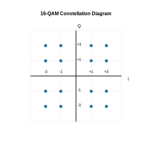
In discrete symbol transmission, I and Q take values from a predefined constellation diagram, where each point represents a unique combination of amplitude and phase.
Constellation Diagrams
A QAM constellation diagram plots the possible states of the signal in the complex plane, with the in-phase component on the x-axis and the quadrature component on the y-axis. For example, 16-QAM uses 16 distinct points, enabling the transmission of 4 bits per symbol.
Spectral Efficiency and Bit Rate
The spectral efficiency η of QAM is given by:
where M is the number of constellation points. For example, 64-QAM (M = 64) achieves 6 bits/s/Hz, while 256-QAM achieves 8 bits/s/Hz.
Error Performance and Signal-to-Noise Ratio (SNR)
The probability of symbol error Pe for an M-QAM system in an additive white Gaussian noise (AWGN) channel is approximated by:
where:
- Q(·) is the Q-function,
- Eb/N0 is the bit energy-to-noise power spectral density ratio.
Applications of QAM
QAM is widely used in modern communication systems due to its high spectral efficiency. Key applications include:
- Digital Cable Television (e.g., 64-QAM, 256-QAM) – Efficiently transmits multiple HD channels over limited bandwidth.
- Wi-Fi (802.11ac/ax) – Uses 256-QAM and higher for increased data rates.
- Fiber-Optic Communications – Coherent optical QAM (e.g., 16-QAM, 64-QAM) enhances long-haul transmission capacity.
- 5G Cellular Networks – Higher-order QAM (up to 1024-QAM) supports ultra-high data rates.
Challenges in QAM Implementation
Despite its advantages, QAM faces several challenges:
- Nonlinear Distortion – High-order QAM is sensitive to amplifier nonlinearities, requiring linearization techniques.
- Phase Noise – Local oscillator instability degrades constellation accuracy.
- Channel Equalization – Multipath fading necessitates adaptive equalization to preserve orthogonality.
4. Orthogonal Frequency Division Multiplexing (OFDM)
4.1 Orthogonal Frequency Division Multiplexing (OFDM)
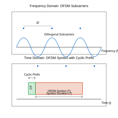
Orthogonal Frequency Division Multiplexing (OFDM) is a multicarrier modulation technique that divides a high-rate data stream into multiple parallel lower-rate substreams, each modulated onto a separate subcarrier. The subcarriers are orthogonal to each other, ensuring minimal interference despite spectral overlap. This property makes OFDM highly efficient in bandwidth utilization and robust against multipath fading.
Mathematical Foundation
The orthogonality condition for subcarriers in OFDM is expressed as:
where T is the symbol duration, and fk, fl are the frequencies of the k-th and l-th subcarriers, respectively. The subcarrier spacing Δf is chosen such that:
ensuring orthogonality over the symbol period.
OFDM System Model
The baseband OFDM signal s(t) for a block of N symbols is given by:
where Xk is the complex symbol modulating the k-th subcarrier. In practice, this is implemented digitally using the Inverse Discrete Fourier Transform (IDFT):
The receiver performs a Discrete Fourier Transform (DFT) to recover the transmitted symbols:
Cyclic Prefix and Robustness to Multipath
To mitigate intersymbol interference (ISI) caused by multipath propagation, OFDM prepends a cyclic prefix (CP) to each symbol. The CP is a copy of the last L samples of the symbol appended to its beginning, ensuring that the linear convolution with the channel impulse response becomes circular convolution. The length of the CP must exceed the maximum delay spread of the channel.
Spectral Efficiency and Advantages
OFDM achieves high spectral efficiency due to overlapping subcarriers, unlike traditional Frequency Division Multiplexing (FDM). Key advantages include:
- Robustness to frequency-selective fading: Each subcarrier experiences flat fading, simplifying equalization.
- Efficient implementation: Fast Fourier Transform (FFT) algorithms reduce computational complexity.
- Scalability: Adaptive modulation and coding can be applied per subcarrier.
Practical Applications
OFDM is widely adopted in modern communication systems:
- Wi-Fi (IEEE 802.11a/g/n/ac/ax): Uses OFDM with varying subcarrier counts (e.g., 52 subcarriers in 802.11a).
- 4G LTE and 5G NR: Employs OFDMA (Orthogonal Frequency Division Multiple Access) for downlink and SC-FDMA for uplink.
- Digital broadcasting (DVB-T, DAB): Resilient to multipath in terrestrial transmission.
Challenges and Mitigations
Despite its advantages, OFDM faces several challenges:
- High Peak-to-Average Power Ratio (PAPR): Requires power amplifiers with high linearity. Solutions include clipping, companding, and tone reservation.
- Sensitivity to carrier frequency offset: Causes intercarrier interference (ICI). Pilot-assisted synchronization is used for compensation.
- Phase noise: Degrades orthogonality. Advanced oscillators and phase-tracking algorithms are employed.
4.2 Spread Spectrum Techniques
Spread spectrum techniques are a class of modulation methods that distribute signal energy over a bandwidth significantly wider than the minimum required for transmission. This approach enhances resistance to interference, jamming, and eavesdropping while enabling multiple access communication. Two primary methods dominate: Direct Sequence Spread Spectrum (DSSS) and Frequency Hopping Spread Spectrum (FHSS).
Direct Sequence Spread Spectrum (DSSS)
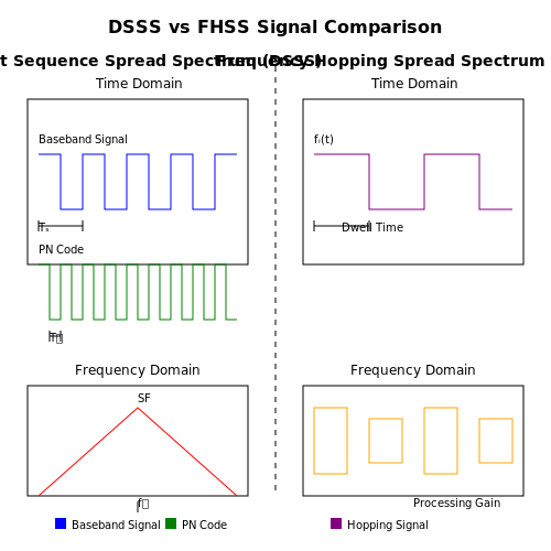
In DSSS, the baseband signal is multiplied by a high-rate pseudorandom noise (PN) code, spreading its spectrum. The PN code consists of chips, with each chip duration much shorter than the symbol period. The spreading factor (SF), defined as:
where \(T_s\) is the symbol duration, \(T_c\) is the chip duration, \(R_c\) is the chip rate, and \(R_s\) is the symbol rate. The receiver correlates the received signal with the same PN code to despread it, recovering the original signal while suppressing narrowband interference.
Mathematically, the transmitted DSSS signal \(s(t)\) is:
where \(d(t)\) is the data signal, \(p(t)\) is the PN code, and \(f_c\) is the carrier frequency. The processing gain \(G_p\) quantifies interference rejection:
Frequency Hopping Spread Spectrum (FHSS)
FHSS rapidly switches the carrier frequency among many channels in a pseudorandom sequence synchronized between transmitter and receiver. The hopping pattern is determined by a PN generator, and the dwell time on each frequency is typically shorter than the coherence time of potential interferers. FHSS is categorized as:
- Slow Hopping: Multiple symbols transmitted per hop.
- Fast Hopping: Multiple hops per symbol.
The instantaneous bandwidth per hop is narrow, but the aggregate bandwidth spans all possible hop frequencies. The hopping sequence must be known at the receiver for coherent demodulation. The transmitted FHSS signal is:
where \(f_i(t)\) cycles through the hop set according to the PN sequence.
Comparison and Applications
DSSS excels in environments with narrowband interference due to its processing gain, while FHSS is robust against frequency-selective fading and follows regulatory requirements for average power spectral density. Practical applications include:
- Wireless LANs (IEEE 802.11): DSSS in early Wi-Fi, FHSS in Bluetooth.
- Military Communications: Anti-jamming and low probability of intercept (LPI).
- Cellular Networks (CDMA): DSSS underpins code-division multiple access.
Time Hopping and Hybrid Methods
Less common than DSSS and FHSS, Time Hopping Spread Spectrum (THSS) transmits short pulses in pseudorandom time slots, combining aspects of pulse-position modulation and spread spectrum. Hybrid systems, such as DSSS/FHSS, merge techniques to leverage their combined advantages—for instance, in ultra-wideband (UWB) communications.
The choice of spread spectrum method depends on the trade-offs between complexity, spectral efficiency, and robustness. Modern implementations often integrate these techniques with error correction coding and adaptive filtering to further enhance performance.
4.3 Adaptive Modulation
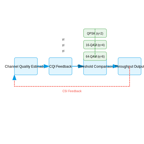
Adaptive modulation dynamically adjusts modulation schemes and coding rates based on real-time channel conditions to maximize spectral efficiency while maintaining an acceptable bit error rate (BER). This technique is fundamental in modern wireless systems like 5G, Wi-Fi 6, and satellite communications where channel quality fluctuates due to fading, interference, or mobility.
Channel State Information (CSI) Feedback
The system continuously estimates the channel quality using pilot signals or preamble sequences. The receiver quantizes this information into a Channel Quality Indicator (CQI), typically transmitted via a feedback loop. For a Rayleigh fading channel, the Signal-to-Noise Ratio (SNR) γ follows an exponential distribution:
where γ̄ is the average SNR. The CQI maps γ to discrete modulation and coding scheme (MCS) levels.
Threshold-Based Switching
Adaptive systems predefine SNR thresholds {γ0, γ1, ..., γN} for MCS transitions. For N possible schemes, the spectral efficiency η(γ) becomes:
where ηn is the bits/symbol for scheme n, and 1 is the indicator function. The optimal thresholds minimize BER while maximizing throughput.
Practical Implementation
Modern standards implement adaptive modulation through:
- Link adaptation algorithms (e.g., LTE's Outer Loop Link Adaptation)
- Hybrid ARQ with incremental redundancy
- MIMO precoding adjustments based on CSI
In Wi-Fi 6 (802.11ax), the Modulation and Coding Scheme (MCS) table extends to 1024-QAM with SNR thresholds adjusted for OFDMA subcarriers. The spectral efficiency gain over static modulation can exceed 300% in time-varying channels.
Performance Analysis
The average throughput Ravg under adaptive modulation with N schemes is:
where B is the channel bandwidth. This shows the trade-off between higher-order modulations (increasing ηn) and their stricter SNR requirements (reducing the probability term).
5. Modulation in Wireless Communication Systems
5.1 Modulation in Wireless Communication Systems
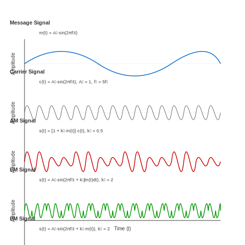
Wireless communication systems rely on modulation to transmit information efficiently over radio frequency (RF) channels. Modulation involves varying one or more properties of a carrier signal—amplitude, frequency, or phase—in accordance with the modulating signal. The choice of modulation technique directly impacts bandwidth efficiency, power consumption, and robustness against noise and interference.
Fundamental Modulation Types
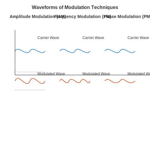
Three primary analog modulation techniques form the basis of wireless communication:
- Amplitude Modulation (AM): The carrier signal's amplitude varies linearly with the message signal while its frequency and phase remain constant. The modulated signal is expressed as:
where \( A_c \) is the carrier amplitude, \( k_a \) is the amplitude sensitivity, \( m(t) \) is the message signal, and \( f_c \) is the carrier frequency.
- Frequency Modulation (FM): The carrier frequency deviates proportionally to the message signal. The instantaneous frequency \( f_i(t) \) is given by:
where \( k_f \) is the frequency sensitivity. The resulting FM signal is:
- Phase Modulation (PM): The carrier phase varies with the message signal:
where \( k_p \) is the phase sensitivity. PM is closely related to FM, with the key difference being the dependence on the message signal's instantaneous value rather than its integral.
Digital Modulation Techniques
Modern wireless systems predominantly use digital modulation due to its superior noise immunity and compatibility with digital signal processing. Key techniques include:
- Amplitude Shift Keying (ASK): The carrier amplitude switches between discrete levels representing binary data. The simplest form is Binary ASK (BASK):
where \( m(t) \) takes values 0 or 1.
- Frequency Shift Keying (FSK): The carrier frequency shifts between predefined values. For Binary FSK (BFSK):
- Phase Shift Keying (PSK): The carrier phase changes abruptly to represent data symbols. Binary PSK (BPSK) uses two phases separated by 180°:
Higher-order modulation schemes like Quadrature PSK (QPSK) and Quadrature Amplitude Modulation (QAM) increase spectral efficiency by encoding multiple bits per symbol.
Performance Metrics
The effectiveness of a modulation scheme is evaluated through several key parameters:
- Bandwidth Efficiency (η): Measured in bits per second per Hertz (bps/Hz), it quantifies how efficiently a modulation scheme utilizes bandwidth:
where \( R_b \) is the bit rate and \( B \) is the bandwidth.
- Power Efficiency: The required \( E_b/N_0 \) (energy per bit to noise power spectral density ratio) to achieve a target bit error rate (BER).
- Robustness: Resistance to channel impairments like multipath fading and interference.
Advanced Modulation Schemes
Modern wireless standards employ sophisticated modulation techniques to optimize performance:
- Orthogonal Frequency Division Multiplexing (OFDM): Divides the available spectrum into multiple orthogonal subcarriers, each modulated at a low symbol rate. This provides resilience against frequency-selective fading and inter-symbol interference (ISI).
- Spread Spectrum Techniques: Including Direct Sequence Spread Spectrum (DSSS) and Frequency Hopping Spread Spectrum (FHSS), these methods spread the signal over a wider bandwidth to enhance security and interference rejection.
The selection of modulation technique in practical systems involves trade-offs between bandwidth efficiency, power efficiency, implementation complexity, and robustness to channel conditions. For instance, 5G networks utilize adaptive modulation and coding (AMC) to dynamically adjust the modulation scheme based on real-time channel quality.
5.2 Modulation in Optical Communication
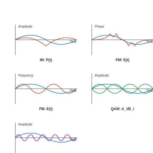
Optical communication systems rely on modulation techniques to encode information onto light waves, typically in the infrared or visible spectrum. The primary methods include intensity modulation (IM), phase modulation (PM), and frequency modulation (FM), each with distinct advantages in bandwidth efficiency, noise resilience, and implementation complexity.
Intensity Modulation (IM)
Intensity modulation, the most common technique in fiber-optic systems, varies the optical power of the light source (e.g., laser diode or LED) in proportion to the input signal. The modulated signal can be expressed as:
where P(t) is the instantaneous optical power, P0 is the average power, m is the modulation index (0 ≤ m ≤ 1), and s(t) is the normalized input signal. IM is straightforward to implement but suffers from susceptibility to nonlinearities and chromatic dispersion.
Phase and Frequency Modulation
Phase modulation encodes data in the phase of the optical carrier, while frequency modulation varies the carrier frequency. The electric field of a phase-modulated signal is:
Here, Δϕ is the phase deviation, and ωc is the carrier frequency. FM is a derivative of PM, where the frequency shift Δf is proportional to the input signal. Both techniques offer superior noise immunity compared to IM but require coherent detection, increasing receiver complexity.
Advanced Techniques
Quadrature Amplitude Modulation (QAM)
Optical QAM combines amplitude and phase modulation to achieve higher spectral efficiency. A 16-QAM signal, for example, encodes 4 bits per symbol by varying both amplitude and phase in quadrature:
where Ai and Bi are discrete amplitude levels. QAM is widely used in high-capacity coherent optical systems.
Orthogonal Frequency-Division Multiplexing (OFDM)
Optical OFDM divides the signal into multiple orthogonal subcarriers, each modulated independently. The time-domain OFDM signal is:
where Xk are the complex symbols, and Δf is the subcarrier spacing. OFDM mitigates inter-symbol interference in dispersive channels.
Practical Considerations
Real-world implementations must account for:
- Chromatic dispersion: Compensated via dispersion-shifted fibers or digital signal processing.
- Nonlinear effects: Including self-phase modulation and four-wave mixing, which limit power levels.
- Detection methods: Direct detection for IM versus coherent detection for PM/FM.
Modern systems often employ digital signal processing (DSP) to correct impairments and enhance performance, enabling terabit-scale data transmission over long-haul fiber networks.
5.3 Trade-offs in Modulation Selection
Selecting an optimal modulation scheme involves balancing multiple competing factors, including spectral efficiency, power efficiency, robustness to noise, and implementation complexity. The choice depends on the specific application constraints, such as available bandwidth, permissible transmit power, and channel conditions.
Spectral Efficiency vs. Power Efficiency
Higher-order modulation schemes like 64-QAM or 256-QAM achieve greater spectral efficiency by encoding more bits per symbol, allowing higher data rates within the same bandwidth. However, they require a higher signal-to-noise ratio (SNR) to maintain the same bit error rate (BER) as lower-order schemes like QPSK or BPSK. The Shannon-Hartley theorem defines the theoretical limit:
where C is channel capacity (bits/s), B is bandwidth (Hz), and S/N is the SNR. In practice, higher-order modulations approach this limit but demand increased transmit power or improved channel conditions.
Robustness to Noise and Interference
Non-coherent modulation techniques like FSK or DPSK sacrifice spectral efficiency for simpler receiver implementation and resilience to phase noise. This makes them suitable for low-power IoT devices or high-mobility scenarios where carrier recovery is challenging. Conversely, coherent schemes like QAM or PSK offer superior spectral efficiency but require precise synchronization.
Implementation Complexity
The computational cost of modulation/demodulation scales with constellation density. A 1024-QAM system requires:
- High-resolution DAC/ADC converters (≥12 bits)
- Precise linear amplifiers
- Advanced equalization algorithms
For battery-constrained devices, the energy consumption of these components may outweigh the benefits of higher data rates.
Case Study: 5G NR Modulation
5G New Radio dynamically selects modulation (QPSK to 256-QAM) based on channel quality indicators (CQI). In urban macro-cells with high SNR, 256-QAM maximizes throughput. For cell-edge users, QPSK ensures reliable connectivity despite lower spectral efficiency. This adaptive approach demonstrates the practical application of modulation trade-offs.
Nonlinear Channel Considerations
In satellite communications, constant envelope modulations like GMSK are preferred over QAM because they tolerate amplifier nonlinearities without spectral regrowth. The trade-off is quantified through the modulation error ratio (MER):
This metric captures both noise and distortion effects, guiding modulation selection in nonlinear channels.