Ideal Transformers
1. Definition and Core Assumptions
Ideal Transformers: Definition and Core Assumptions
An ideal transformer is a theoretical model of a transformer that exhibits perfect coupling between its primary and secondary windings with no energy losses. It serves as a foundational concept in electrical engineering, providing a simplified framework for analyzing transformer behavior before considering real-world imperfections.
Fundamental Definition
An ideal transformer is defined by the following voltage-current relationship between its primary (input) and secondary (output) sides:
where V1 and V2 are the primary and secondary voltages, I1 and I2 are the primary and secondary currents, N1 and N2 are the number of turns in the primary and secondary windings, and a is the turns ratio.
Core Assumptions
The ideal transformer model makes several critical assumptions:
- Perfect coupling (k = 1): All magnetic flux generated by the primary winding links completely with the secondary winding, and vice versa.
- Zero winding resistance: Both primary and secondary windings exhibit no ohmic losses (R1 = R2 = 0).
- Infinite core permeability: The core material requires negligible magnetizing current to establish flux (μ → ∞).
- No leakage flux: All magnetic flux remains confined to the core with no stray fields.
- No core losses: The model neglects both hysteresis and eddy current losses in the magnetic core.
- Linear B-H characteristics: The core operates in its linear region without saturation effects.
Power Conservation
As a consequence of these assumptions, an ideal transformer exhibits perfect power transfer between windings:
This relationship holds instantaneously, with no energy storage in the transformer. The apparent power remains conserved across the windings, making the ideal transformer a lossless device.
Impedance Transformation
The ideal transformer provides impedance scaling by the square of the turns ratio. For a load impedance ZL connected to the secondary, the reflected impedance Zin at the primary is:
This property is particularly valuable in impedance matching applications, where maximum power transfer between circuits with different impedance levels is required.
Practical Relevance
While no physical transformer can meet all ideal assumptions, the model provides:
- A first-order approximation for transformer behavior in many circuit analyses
- A benchmark for evaluating real transformer performance through deviation from ideal characteristics
- A conceptual foundation for understanding more complex transformer models
Engineers often begin with ideal transformer analysis before incorporating parasitic elements like winding resistances, leakage inductances, and core losses in more advanced models.
1.2 Key Electrical Properties
Voltage and Current Relationships
An ideal transformer enforces strict proportionality between primary and secondary voltages and currents. For a transformer with Np primary turns and Ns secondary turns, the voltage transformation ratio a is defined as:
The voltage and current relationships are then given by:
These equations assume:
- Perfect magnetic coupling (no leakage flux)
- Zero winding resistance
- Infinite core permeability
- Negligible core losses (hysteresis and eddy currents)
Power Conservation
In an ideal transformer, power is perfectly conserved between primary and secondary windings. The apparent power equality holds:
Expressed in terms of voltage and current:
where I* denotes the complex conjugate of current. For purely resistive loads, this simplifies to:
Impedance Transformation
An ideal transformer modifies impedance as seen from the primary side according to:
where Zp is the apparent impedance at the primary terminals and Zs is the actual load impedance connected to the secondary. This property is crucial for impedance matching applications in RF and power systems.
Frequency Independence
Unlike real transformers, ideal transformers exhibit no frequency-dependent behavior. The voltage ratio remains constant across all frequencies, and there are no parasitic capacitances or inductances to create frequency-selective effects.
Phase Relationships
The phase angle between primary and secondary voltages depends on the winding configuration:
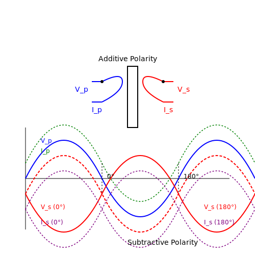
- Additive polarity: Primary and secondary voltages are in phase
- Subtractive polarity: Primary and secondary voltages are 180° out of phase
For three-phase transformers, the phase displacement follows standard vector group notations (e.g., Dyn11, YNd1).
Practical Limitations and Deviations
While ideal transformer theory provides fundamental relationships, real transformers deviate due to:
- Finite core permeability leading to magnetizing current
- Winding resistances causing voltage drops
- Leakage reactances affecting voltage regulation
- Core losses generating heat
- Saturation effects at high fluxes
These non-ideal characteristics become particularly important in high-power applications where efficiency and thermal management are critical.
Ideal vs. Real Transformers: Core Differences
Definition and Assumptions
An ideal transformer is a theoretical construct that assumes perfect magnetic coupling between primary and secondary windings, zero energy losses, and infinite core permeability. The governing equations for an ideal transformer are derived from Faraday's law of induction and Ampere's circuital law under these simplifying assumptions:
where a is the turns ratio, V represents voltage, I represents current, and N denotes the number of turns in each winding.
Non-Ideal Behavior in Physical Transformers
Real transformers deviate from ideal behavior due to several physical limitations:
- Core losses: Hysteresis and eddy currents in the ferromagnetic core dissipate energy as heat. Hysteresis loss is proportional to the area of the B-H curve, while eddy current loss follows:
where ke is a material constant, f is frequency, Bmax is peak flux density, and t is lamination thickness.
- Winding resistance: Finite conductivity of copper windings causes ohmic losses (I²R).
- Leakage flux: Imperfect coupling results in flux that doesn't link both windings, modeled by leakage inductance.
- Finite permeability: Real cores require magnetizing current to establish flux, creating a small phase shift.
Equivalent Circuit Representation
The non-ideal transformer can be modeled with the following circuit elements added to the ideal case:
Where R1 and R2 represent winding resistances, Xm models the magnetizing reactance, and leakage reactances are omitted for clarity.
Performance Metrics Comparison
The table below quantifies typical deviations from ideal behavior in medium-power distribution transformers:
| Parameter | Ideal Transformer | Real Transformer (Typical) |
|---|---|---|
| Efficiency | 100% | 95-99% |
| Voltage Regulation | 0% | 2-5% |
| No-Load Current | 0 A | 1-3% of rated |
Practical Design Implications
Engineers must account for non-ideal effects when:
- Specifying cooling requirements based on total losses
- Designing voltage regulation systems to compensate for impedance drops
- Selecting core materials to minimize hysteresis losses at operating frequencies
- Implementing protective relaying that must distinguish between magnetizing inrush currents and fault conditions
The deviation from ideal behavior becomes particularly significant in high-frequency power electronics applications, where skin and proximity effects exacerbate winding losses, and core losses dominate at elevated frequencies.
2. Voltage and Current Relationships
2.1 Voltage and Current Relationships
Fundamental Principles
In an ideal transformer, the voltage and current relationships between the primary and secondary windings are governed by Faraday's law of induction and the principle of conservation of energy. The transformer operates under the assumption of perfect coupling (no leakage flux), zero winding resistance, and no core losses. The turns ratio a, defined as the ratio of secondary turns N2 to primary turns N1, is the key parameter:
Voltage Transformation
The primary voltage V1 and secondary voltage V2 are related by the turns ratio. For sinusoidal excitation, the instantaneous voltage relationship is derived from Faraday's law:
In phasor notation for steady-state analysis, this becomes:
Current Transformation
The current relationship follows from power conservation (input power = output power in an ideal transformer). For instantaneous currents:
Expressed in terms of phasor currents and turns ratio:
Impedance Transformation
The transformer also modifies the apparent impedance. A load impedance ZL connected to the secondary appears as Z' at the primary:
Practical Implications
These relationships enable voltage stepping for power transmission (high-voltage/low-current for reduced I2R losses) and impedance matching in RF systems. In three-phase systems, delta-wye transformer configurations combine voltage transformation with phase shift.
2.2 Turns Ratio and Its Impact
Fundamental Definition
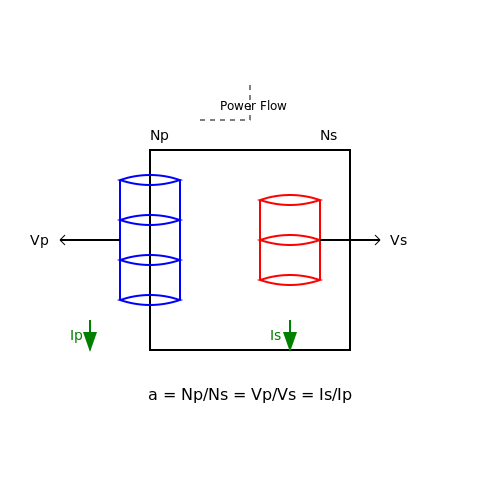
The turns ratio a of an ideal transformer is defined as the ratio of the number of turns in the primary winding (Np) to the number of turns in the secondary winding (Ns):
This ratio directly governs the voltage and current transformation between the primary and secondary sides. In an ideal transformer, where losses are negligible, the turns ratio is the sole determinant of the input-output relationship.
Voltage and Current Transformation
For an ideal transformer, the voltage transformation follows directly from Faraday's law of induction. The primary voltage (Vp) and secondary voltage (Vs) are related by:
Similarly, due to power conservation (Pp = Ps), the current transformation is inversely proportional to the turns ratio:
Impedance Transformation
The turns ratio also affects the impedance seen by the primary side. If a load impedance ZL is connected to the secondary, the equivalent impedance Z' reflected to the primary is:
This property is crucial in impedance matching applications, such as in RF systems or audio amplifiers, where maximum power transfer is desired.
Practical Considerations
While ideal transformers assume perfect coupling and no losses, real-world transformers exhibit:
- Leakage inductance: Some flux does not link both windings, causing voltage drops.
- Winding resistance: Resistive losses in the copper windings.
- Core losses: Hysteresis and eddy current losses in the magnetic core.
Despite these non-idealities, the turns ratio remains the dominant factor in determining transformer behavior, making it a critical design parameter.
Applications in Power Systems
In power distribution, step-up transformers (a < 1) increase voltage to reduce transmission losses, while step-down transformers (a > 1) decrease voltage for safe consumer use. For example, a 10:1 step-down transformer converts 2400 V to 240 V with a turns ratio of 10.
2.3 Power Transfer and Efficiency
Power Conservation in Ideal Transformers
In an ideal transformer, power transfer occurs without losses, meaning the input power (Pin) equals the output power (Pout). This is derived from the conservation of energy principle. For sinusoidal steady-state conditions, the complex power at the primary (S1) and secondary (S2) must satisfy:
where V1, I1 are the primary voltage and current, and V2, I2 are the secondary voltage and current. The asterisk denotes the complex conjugate. The real power (P) and reactive power (Q) are thus preserved:
Voltage and Current Relationships
The turns ratio (a = N1/N2) directly governs the voltage and current scaling:
Combining these with the power equality V1I1 = V2I2, it follows that the apparent power (|S|) is invariant across the transformer. This property is critical for impedance matching applications, where maximum power transfer is achieved when the load impedance (ZL) is reflected to the primary as ZL' = a²ZL.
Efficiency and Practical Considerations
While ideal transformers exhibit 100% efficiency, real transformers incur losses due to:
- Copper losses (I²R): Resistive heating in windings.
- Core losses: Hysteresis and eddy currents in the magnetic material.
- Leakage flux: Imperfect coupling between windings.
The efficiency (η) of a practical transformer is defined as:
For high-power applications (e.g., grid transformers), efficiencies exceed 98%, achieved through laminated silicon steel cores and low-resistance windings. In contrast, high-frequency transformers (e.g., switch-mode power supplies) prioritize reduced core losses via ferrite materials.
Case Study: Power Distribution Networks
Ideal transformer theory underpins the design of step-up and step-down substations. For instance, a 138 kV transmission line might use a step-down transformer with a = 10 to deliver 13.8 kV to local distribution grids. The absence of reactive power losses in the ideal case simplifies load flow analysis, though real-world models must account for impedance and admittance matrices.
3. Impedance Matching
3.1 Impedance Matching
In an ideal transformer, impedance matching is achieved by exploiting the turns ratio to maximize power transfer between a source and a load. The primary and secondary impedances (ZP and ZS) relate quadratically to the turns ratio N = NP/NS:
This relationship arises from the conservation of power and the voltage/current scaling properties of transformers. For a source impedance Zsrc and load impedance Zload, maximum power transfer occurs when:
Derivation of Impedance Scaling
Starting with the ideal transformer properties:
The impedance on the primary side ZP is:
Practical Applications
Impedance matching is critical in:
- RF systems: Antenna feedlines require matching to minimize reflections (e.g., 50 Ω to 75 Ω transformers).
- Audio engineering: Matching microphone/output impedances to prevent signal degradation.
- Power electronics: Optimizing coupling between amplifier stages and loads.
Case Study: RF Transformer
A 4:1 impedance ratio transformer (N = 2) converts a 200 Ω antenna to 50 Ω for coaxial cable transmission. The power transfer efficiency is theoretically 100% in the ideal case, with no reflected waves.
3.2 Step-Up and Step-Down Configurations
In an ideal transformer, the voltage transformation ratio is determined by the turns ratio Np/Ns, where Np and Ns are the number of turns in the primary and secondary windings, respectively. The relationship between the primary voltage Vp and secondary voltage Vs is given by:
Step-Up Transformers
A step-up transformer increases the secondary voltage relative to the primary voltage by having Ns > Np. This configuration is essential in power transmission systems, where high-voltage transmission minimizes resistive losses (I2R) over long distances. For instance, a transformer with a turns ratio of 1:10 will convert 1 kV at the primary to 10 kV at the secondary.
In practice, step-up transformers are used at power generation stations to elevate voltage levels before transmission. The high-voltage side typically employs thicker insulation and specialized winding techniques to handle the increased electrical stress.
Step-Down Transformers
Conversely, a step-down transformer reduces the secondary voltage by having Ns < Np. This configuration is widely used in power distribution networks to bring transmission-level voltages (e.g., 138 kV) down to safer levels (e.g., 480 V or 120 V) for industrial and residential use.
Step-down transformers must account for load variations, ensuring stable output voltage under varying current demands. Ferromagnetic core materials with high permeability are often used to enhance flux linkage and efficiency.
Power Conservation in Ideal Transformers
Assuming an ideal transformer (no losses), power conservation dictates that input power equals output power:
Thus, current transformation follows an inverse relationship with voltage:
This principle ensures that while voltage is stepped up or down, current adjusts proportionally to maintain energy balance.
Practical Considerations
Real-world transformers deviate from ideal behavior due to:
- Core losses: Hysteresis and eddy currents dissipate energy as heat.
- Copper losses: Resistive heating in windings (I2R).
- Leakage flux: Imperfect coupling between windings reduces efficiency.
Advanced designs mitigate these losses through laminated cores, high-conductivity windings, and precise geometric alignment of coils.
3.3 Phasor Diagrams for AC Analysis
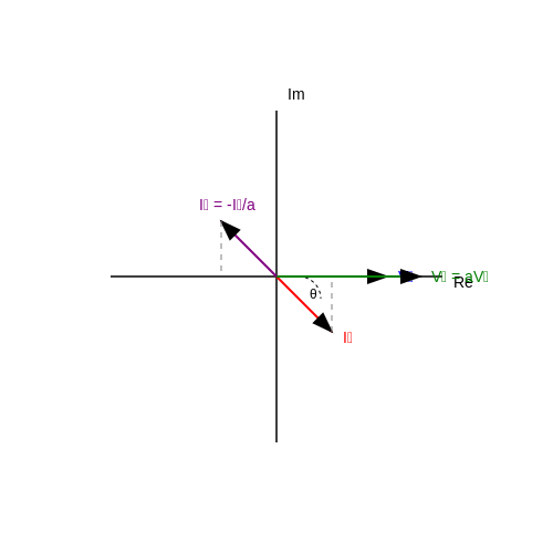
Phasor diagrams provide a graphical representation of sinusoidal voltages and currents in AC circuits, simplifying the analysis of ideal transformers under steady-state conditions. By converting time-domain waveforms into complex phasors, phase relationships between primary and secondary quantities become immediately apparent.
Phasor Representation of Transformer Quantities
For an ideal transformer with turns ratio a = N₁/N₂, the primary and secondary voltages and currents are related as:
where $$\tilde{V}_1$$ and $$\tilde{V}_2$$ are the primary and secondary voltage phasors, and $$\tilde{I}_1$$ and $$\tilde{I}_2$$ are the current phasors. In an ideal transformer, these phasors maintain precise phase alignment:
- The primary and secondary voltages are in phase for the dot convention shown.
- The primary and secondary currents are 180° out of phase due to power conservation.
Constructing the Phasor Diagram
Consider an ideal transformer supplying a load with impedance Z_L = R + jX. The phasor diagram construction proceeds as follows:
- Reference Phasor: Typically, the secondary voltage $$\tilde{V}_2$$ is chosen as the reference (0° phase).
- Load Current: The secondary current $$\tilde{I}_2$$ lags $$\tilde{V}_2$$ by angle θ = tan⁻¹(X/R) for inductive loads.
- Primary Voltage: $$\tilde{V}_1$$ is scaled by a and aligned with $$\tilde{V}_2$$.
- Primary Current: $$\tilde{I}_1$$ is scaled by 1/a and inverted (180° phase shift) relative to $$\tilde{I}_2$$.
Power Factor Considerations
The phasor diagram clearly shows that the power factor angle θ is identical on both primary and secondary sides:
where P is the real power and |S| is the apparent power. For an ideal transformer, the complex power is conserved:
Practical Applications
Phasor diagrams are indispensable for:
- Analyzing voltage regulation in transformer systems
- Determining phase shifts in polyphase transformer connections
- Troubleshooting power factor correction circuits
- Visualizing the effects of harmonic distortions
4. Non-Ideal Effects in Real-World Transformers
4.1 Non-Ideal Effects in Real-World Transformers
Core Non-Ideal Phenomena
Real-world transformers deviate from ideal behavior due to several physical limitations. The primary non-ideal effects include:
- Winding resistance - Copper losses in primary and secondary windings (I²R dissipation)
- Leakage flux - Magnetic flux that doesn't couple both windings
- Core losses - Hysteresis and eddy current losses in the magnetic material
- Finite magnetizing current - Current required to establish core flux
- Parasitic capacitance - Interwinding and layer-to-layer capacitance effects
Mathematical Modeling of Losses
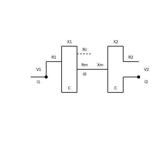
The equivalent circuit of a non-ideal transformer incorporates these effects through additional circuit elements:
Where:
- R₁, R₂ represent winding resistances
- X₁, X₂ model leakage reactances
- I₀ is the magnetizing current
- Prime notation (') denotes quantities referred to the primary
Frequency-Dependent Effects
Transformer behavior changes significantly with frequency due to:
The skin depth (δ) phenomenon causes current crowding at high frequencies, increasing effective resistance. Core losses follow Steinmetz's equation:
Practical Design Considerations
Transformer designers must balance competing requirements:
- Core selection - Laminations vs. ferrite for target frequency range
- Window utilization factor - Typically 0.3-0.6 for power transformers
- Temperature rise - Dictates maximum flux density and current density
The regulation percentage quantifies voltage drop under load:
High-Frequency Behavior
Above 10kHz, parasitic effects dominate:
- Winding capacitance forms self-resonant points
- Proximity effect increases AC resistance
- Core materials exhibit permeability roll-off
The critical frequency where capacitive reactance equals leakage reactance:
4.2 Core Saturation and Losses
Magnetic Saturation in Transformer Cores
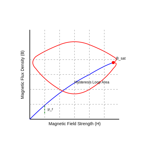
The magnetic flux density B in a transformer core follows the nonlinear B-H curve of the core material. As the magnetizing current increases, the core approaches saturation, where further increases in H yield diminishing returns in B. The saturation flux density Bsat is a material property, typically around 1.5–2.0 T for silicon steel and up to 0.6 T for ferrites.
Beyond Bsat, the relative permeability μr drops sharply, increasing the magnetizing current required to sustain the same flux. This leads to excessive core losses and potential overheating.
Core Losses: Hysteresis and Eddy Currents
Core losses consist of two primary components: hysteresis losses and eddy current losses.
Hysteresis Losses
Hysteresis loss results from the energy dissipated as the magnetic domains in the core material realign with the alternating magnetic field. The area enclosed by the B-H loop represents the energy lost per cycle. For a sinusoidal excitation, hysteresis loss Ph is given by:
where kh is the hysteresis constant, f is the frequency, Bm is the peak flux density, and n (typically 1.6–2.0) depends on the material.
Eddy Current Losses
Eddy currents are induced circulating currents within the core due to time-varying flux. These currents generate resistive heating (I²R losses). The eddy current loss Pe is expressed as:
where ke is the eddy current constant, and t is the lamination thickness. To minimize eddy currents, transformer cores are laminated with thin, insulated layers.
Practical Implications of Core Saturation
In power transformers, operating near saturation increases harmonic distortion, reduces efficiency, and can cause protective relays to trip. Designers must ensure:
- The operating flux density remains below Bsat under worst-case conditions.
- The core material is selected for low hysteresis and eddy current losses.
- The core geometry minimizes flux leakage and hot spots.
Advanced Core Materials
Modern high-frequency transformers often use nanocrystalline alloys or powdered cores, which exhibit lower losses and higher saturation thresholds than traditional silicon steel. These materials enable compact, high-efficiency designs for switched-mode power supplies and renewable energy systems.
4.3 Frequency Response Considerations
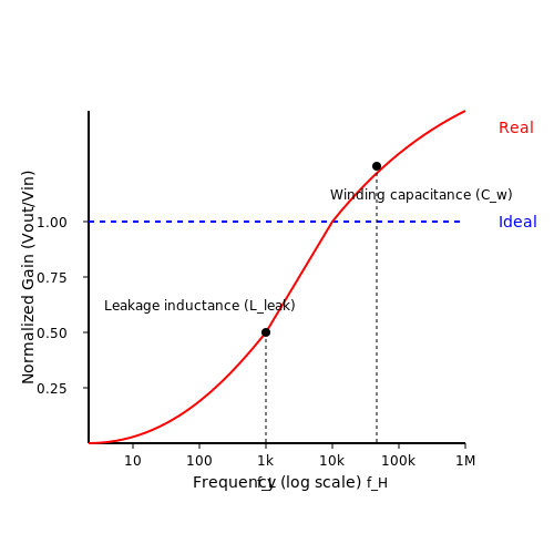
The frequency response of an ideal transformer is inherently flat across all frequencies, as it assumes perfect coupling, zero leakage inductance, and no parasitic capacitance. However, real-world transformers exhibit frequency-dependent behavior due to non-ideal characteristics. The primary factors influencing frequency response include:
- Leakage inductance (Lleak): Causes high-frequency roll-off due to increased reactance (XL = 2πfLleak).
- Winding capacitance (Cw): Introduces a low-pass filter effect, attenuating high frequencies.
- Core losses (Rc): Frequency-dependent hysteresis and eddy current losses reduce efficiency at higher frequencies.
Mathematical Derivation of Frequency Limits
The lower cutoff frequency (fL) is determined by the magnetizing inductance (Lm) and the load resistance (RL):
The upper cutoff frequency (fH) is governed by the leakage inductance and winding capacitance:
For broadband applications, the transformer must operate within the range fL ≪ f ≪ fH to maintain a flat frequency response.
Practical Implications
In power systems, transformers are designed for a specific frequency (e.g., 50/60 Hz), where fL and fH are far from the operating point. However, in audio or RF applications, frequency response deviations introduce signal distortion. For example:
- Audio transformers: Must maintain flat response from 20 Hz to 20 kHz, requiring careful minimization of Lleak and Cw.
- RF transformers: Operate at MHz-GHz ranges, where parasitic effects dominate. Ferrite cores and interleaved windings are used to extend fH.
Case Study: Wideband Transformer Design
A common technique to improve high-frequency response is transmission-line transformer design, where windings are treated as transmission lines. The characteristic impedance (Z0) must match the load to minimize reflections:
This approach is widely used in baluns and impedance-matching networks for antennas.
5. Recommended Textbooks
5.1 Recommended Textbooks
- FUNDAMENTALS OF ELECTRIC POWER ENGINEERING - Wiley Online Library — 5.3.3 Mutual Inductors and the Ideal Transformer, 146 5.3.4 Systems Containing Ideal Transformers: Magnetically Coupled Circuits, 150 5.4 Simple R-L and R-C Transients, 152 5.5 AC Circuit Analysis, 155 5.5.1 Sinusoidal Functions, 155 5.5.2 Steady-State Behaviour of Linear Circuits Using Phasors, 156 5.5.3 AC Circuit Passive Parameters, 163
- TRANSFORMERS AND INDUCTORS FOR POWER ELECTRONICS - Wiley Online Library — SECTION II TRANSFORMERS 93 Chapter 4 Transformers 95 4.1 Ideal Transformer 96 4.1.1 No Load Conditions 97 4.1.2 Load Conditions 98 4.1.3 Dot Convention 99 4.1.4 Reflected Impedance 100 4.1.5 Summary 101 4.2 Practical Transformer 102 4.2.1 Magnetizing Current and Core Loss 102 4.2.2 Winding Resistance 105 4.2.3 Magnetic Leakage 105 4.2.4 ...
- PDF Principles of Power Electronics - Cambridge University Press & Assessment — 1.1 Power Electronic Circuits 1 1.2 Power Semiconductor Switches 2 1.3 Transformers 5 1.4 Nomenclature 7 1.5 Bibliographies 8 1.6 Problems 8 Part I Form and Function 2 Form and Function: An Overview 11 2.1 Functions of a Power Circuit 11 2.2 AC/DC Converters 13 2.3 DC/DC Converters 18 2.4 AC/AC Converters 20 2.5 Inu ence of Switch ...
- PDF Transformers and - 103.203.175.90:81 — 1.2.2 Faraday's Law of Electromagnetic Induction 5 1.3 Ferromagnetic Materials 7 1.4 Losses in Magnetic Components 10 ... 4.1 Ideal Transformer 96 4.1.1 No Load Conditions 97 4.1.2 Load Conditions 98 4.1.3 Dot Convention 99 ... He received a Best Paper Prize for the IEEE Transactions on Power Elec-tronics in 2000. Prof.
- PDF Practical Electronics Handbook — any means electronic, mechanical, photocopying, recording or otherwise without the prior written permission of ... For information on all Newnes publications visit our web site at books.elsevier.com Typeset by Cepha Ltd Printed and bound in Great Britain 0708091011 10987654321. ... Transformers 51. vi Contents Signal-matching transformers 54 ...
- PDF Chapter 5 Applications of Transformers - Springer — In addition to simulating three-phase transformers, this chapter will introduce high frequency transformers used in power electronic applications [10, 11, 40, 41]. This is of great relevance to a power electronics engineer, as a vast number of dc- dc converters contain transformers and provide isolated outputs. We will begin the
- Electrical Engineering: Fundamentals (De Gruyter Textbook) — 2.7.1 Ideal voltage source / real voltage source 32 2.7.2 Ideal current source / real current source 34 2.7.3 Power adjustment 35 2.8 Voltage divider 36 2.9 The complex calculation in electrical engineering 37 2.9.1 Definitions 37 2.9.2 Application of the complex calculation in AC calculation 40 2.10 Review questions 41 2.11 Exercises 41
- PDF ECE 231: Circuits and Systems I Text book 10th Edition — inductance, and ideal transformers. Prerequisites: Phys 121, Math 112 or Math 133. Specific Course Learning Outcomes (CLO): The student will be able to 1. Develop firm understanding of physical principles behind electric circuit theory. 2. Thoroughly understand operation of passive circuit elements and their specific use in electric circuits. 3.
- PDF Basic Electronics for Scientists and Engineers — Ideal for a one-semester course, this concise textbook covers basic ... 2.9 Transformers 61 Exercises 65 Further reading 67 3 Band theory and diode circuits 68 3.1 The band theory of solids 68 ... A professor of mine once opined that the best working experimentalists tended to
- The Best Online Library of Electrical Engineering Textbooks — Electronics textbooks including: Fundamentals of Electrical Engineering, Electromagnetics, Introduction to Electricity, Magnetism, & Circuits and more. ... transformers, generators, and transmission lines. This book employs the "transmission lines first" approach, in which transmission lines are introduced using a lumped-element equivalent ...
5.2 Research Papers and Articles
- Electronic transformer performance evaluation and its impact on PMU — Research Article Electronic transformer performance evaluation and its impact on PMU ISSN 1751-8687 Received on 16th April 2019 Revised 2nd August 2019 Accepted on 9th October 2019 E-First on 7th November 2019 doi: 10.1049/iet-gtd.2019.0174 www.ietdl.org Jue Li1, Hao Liu1, Kenneth E. Martin2, Jinsong Li1, Tianshu Bi1, Qixun Yang1
- Principles and Test Technology of Electronic Transformers — The primary and secondary sides are completely isolated without any electric connection, which depends on the digital output technology of electronic transformers. Electronic transformers, significant parts in process bus of a smart substation, have attracted much more attention from researchers in recent years and been utilized in the field.
- TRANSFORMERS AND INDUCTORS FOR POWER ELECTRONICS - Wiley Online Library — Chapter 4 Transformers 95 4.1 Ideal Transformer 96 4.1.1 No Load Conditions 97 4.1.2 Load Conditions 98 ... His research interests include high frequency magnetics, power quality, and renewable energy systems. He received a Best Paper Prize for the IEEE Transactions on Power Elec-tronics in 2000. Prof. Hurley is a Fellow of the IEEE.
- Toward the Standardization of Limits to Offset and Noise in Electronic ... — Electronic instrument transformers are expected to play a significant protection and control role in the future smart grids. This paper aims at improving the performance and accuracy of electronic ...
- IET Generation, Transmission & Distribution — The final equivalent electrical circuit for five-legged stacked-core transformer is depicted in Fig. 3c by adding winding resistances and ideal transformers. R H and R L represent the winding resistances of the high and low voltage windings, respectively. The six ideal transformers account for the winding turns ratio and interface the dual ...
- (PDF) Transformer models: an introduction and catalog - ResearchGate — Preprints and early-stage research may not have been peer reviewed yet. ... 2. 5. 2 6 G l o b a l C o n t e x t V i T ... The key insight of the Transformers paper was that, as the title implies ...
- Electronic transformer performance evaluation and its impact on PMU — Research on the transformation characteristics of the electronic transformer and its impact on phasor measurements of PMUs are needed to determine if there are problems in this instrumentation combination. A number of studies have been published on the performance of instrument transformers.
- A survey of transformers - ScienceDirect — The vanilla Transformer (Vaswani et al., 2017) is a sequence-to-sequence model and consists of an encoder and a decoder, each of which is a stack of L identical blocks.Each encoder block is mainly composed of a multi-head self-attention module and a position-wise feed-forward network (FFN). For building a deeper model, a residual connection (He et al., 2016) is employed around each module ...
- Power electronic transformer with adaptive PLL technique for voltage ... — The power electronic transformer (PET) has recently emerged as a type of power converter. It features the basic functions of power conversion and isolation as well as additional functions related to power quality control. A novel PET for a distribution grid called a flexible power distribution unit is proposed in this paper, and the energy exchange mechanism between the network and the load is ...
- An online correction system for electronic voltage transformers — The current calibration techniques of this asset class exhibit several issues including complex real time implementation. In contrary with existing calibration techniques, this paper proposes a new correction system for electronic voltage transformers, which can be conducted online without causing any interruption to the electricity grid.
5.3 Online Resources and Tutorials
- FUNDAMENTALS OF ELECTRIC POWER ENGINEERING - Wiley Online Library — 5.3.3 Mutual Inductors and the Ideal Transformer, 146 5.3.4 Systems Containing Ideal Transformers: Magnetically Coupled Circuits, 150 5.4 Simple R-L and R-C Transients, 152 5.5 AC Circuit Analysis, 155 5.5.1 Sinusoidal Functions, 155 5.5.2 Steady-State Behaviour of Linear Circuits Using Phasors, 156 5.5.3 AC Circuit Passive Parameters, 163
- PDF Renewable and Efficient Electric Power Systems - TU Delft OCW — 1.8 Transformers 36 1.8.1 Ideal Transformers 37 1.8.2 Magnetization Losses 40 Problems 44 2 Fundamentals of Electric Power 51 2.1 Effective Values of Voltage and Current 51 2.2 Idealized Components Subjected to Sinusoidal Voltages 55 2.2.1 Ideal Resistors 55 2.2.2 Idealized Capacitors 57 2.2.3 Idealized Inductors 59 2.3 Power Factor 61
- The Best Online Library of Electrical Engineering Textbooks — Ideal Circuit Elements 3.2; Ideal and Real-World Circuit Elements 3.3; Electric Circuits and Interconnection Laws 3.4; Power Dissipation in Resistor Circuits 3.5; Series and Parallel Circuits 3.6; Equivalent Circuits: Resistors and Sources 3.7; Circuits with Capacitors and Inductors 3.8; The Impedance Concept 3.9; Time and Frequency Domains 3.10
- TRANSFORMERS AND INDUCTORS FOR POWER ELECTRONICS - Wiley Online Library — SECTION II TRANSFORMERS 93 Chapter 4 Transformers 95 4.1 Ideal Transformer 96 4.1.1 No Load Conditions 97 4.1.2 Load Conditions 98 4.1.3 Dot Convention 99 4.1.4 Reflected Impedance 100 4.1.5 Summary 101 4.2 Practical Transformer 102 4.2.1 Magnetizing Current and Core Loss 102 4.2.2 Winding Resistance 105 4.2.3 Magnetic Leakage 105 4.2.4 ...
- Transformers and inductors for power electronics: theory, design and ... — Transformers and inductors for power electronics: theory, design and applications [electronic resource] Responsibility ... Chapter 4 Transformers 95 4.1 Ideal Transformer 96 4.1.1 No Load Conditions 97 4.1.2 Load Conditions 98 4.1.3 Dot Convention 99 4.1.4 Reflected Impedance 100 4.1.5 Summary 101 4.2 Practical Transformer 102 4.2.1 Magnetizing ...
- Principles and Test Technology of Electronic Transformers — The primary and secondary sides are completely isolated without any electric connection, which depends on the digital output technology of electronic transformers. Electronic transformers, significant parts in process bus of a smart substation, have attracted much more attention from researchers in recent years and been utilized in the field.
- PDF EEL 3216 Introduction to Power Systems Homework # 3 — 2. A 20-kVA 8000/277-V distribution transformer has the following resistances and reactances: RP = 32 Ω RS = 0.05 Ω XP = 45 Ω XS = 0.06 Ω RC = 250 kΩ XM= 30 kΩ The excitation branch impedances are given referred to the high-voltage side of
- Electric Transformer and Coupled Inductors | SpringerLink — 12.1.5 Ideal Loaded Transformer. 12.1.6 Ideal Transformer Versus Realistic Transformer: Transformer Terminology. Problem 12.7. For the circuit shown in the following figure, establish the relation between currents i 1 (t) and i 2 (t). Assume the ideal magnetic core. Count the number of turns.
- Home [arena3-chapter1-transformer-interp.streamlit.app] — The first two sections are compulsory, and will guide you through the basic ideas of transformers & mechanistic interpretability. [1.1] Transformer from Scratch will guide you through building a transformer from scratch (and show you how things like transformer training & sampling works), and [1.2] Intro to Mech Interp will guide you through the basics of mechanistic interpretability via the ...
- (PDF) transformer Design guide - Academia.edu — This guide serves as a comprehensive resource for understanding transformer technology within electric power engineering. It addresses all levels of readers—from curious individuals to seasoned experts—by covering fundamental theories, various equipment types, and ancillary topics. ... Electrical and Electronic Engineering, 2012. This paper ...