Network Theorems Applications
1. Ohm's Law and Its Applications
Ohm's Law and Its Applications
Fundamental Formulation
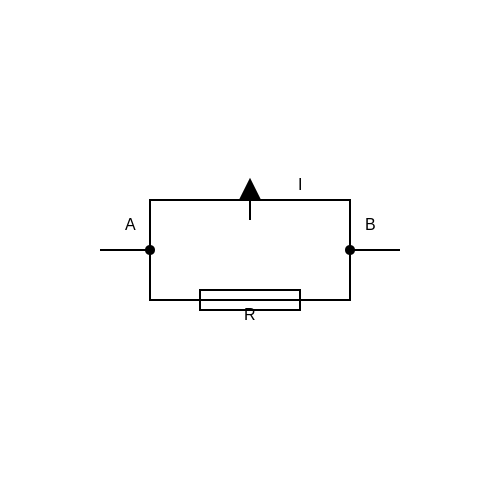
Ohm's Law establishes a linear relationship between voltage V, current I, and resistance R in an electrical circuit. The law is expressed as:
This equation holds under the condition that the conductor's temperature and material properties remain constant. Deviations occur in non-ohmic materials (e.g., semiconductors, diodes) where resistance varies with applied voltage or current.
Derivation from Microscopic Principles
The macroscopic form of Ohm's Law can be derived from the Drude model of electron motion. The current density J relates to the electric field E via:
where σ is conductivity. For a conductor of length L and cross-sectional area A, integrating over the volume yields:
Rearranging gives the familiar form V = IR, with resistance defined as R = L/(σA).
Applications in Circuit Analysis
Ohm's Law serves as the foundation for:
- Nodal and mesh analysis: Enables systematic reduction of complex networks.
- Equivalent resistance calculations: Simplifies series/parallel resistor combinations.
- Power dissipation: Combined with P = VI, predicts heat generation in components.
Case Study: Voltage Divider Design
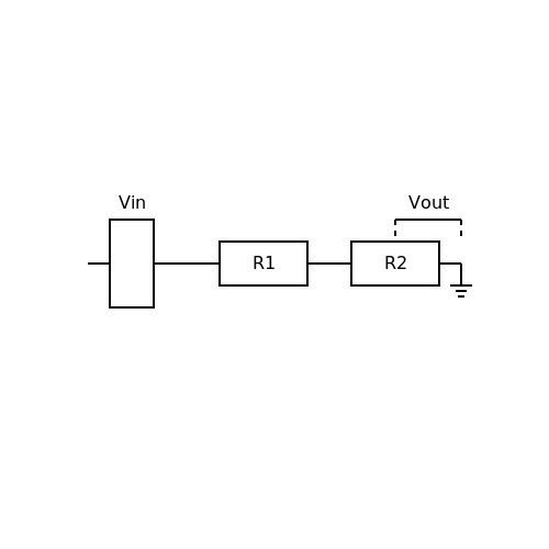
A practical implementation appears in voltage divider circuits:
This relationship assumes negligible load current. For precision applications, the equivalent resistance must account for the Thévenin resistance Rth = R1 || R2.
Non-Ideal Behavior and Limitations
Real-world components exhibit:
- Temperature dependence: Resistance varies as R(T) = R0[1 + α(T - T0)], where α is the temperature coefficient.
- Frequency effects: Skin depth and parasitic reactance dominate at high frequencies.
- Nonlinearity: Observed in thermistors, varistors, and active devices.
Advanced Applications
Modern extensions include:
- Impedance spectroscopy: Generalizes Ohm's Law to complex impedances Z(ω).
- Quantum Hall effect: Provides resistance quantization with RK = h/e2 ≈ 25.812 kΩ.
- Superconductivity: Zero resistance below critical temperature Tc.
Kirchhoff's Laws: Current and Voltage
Fundamental Principles
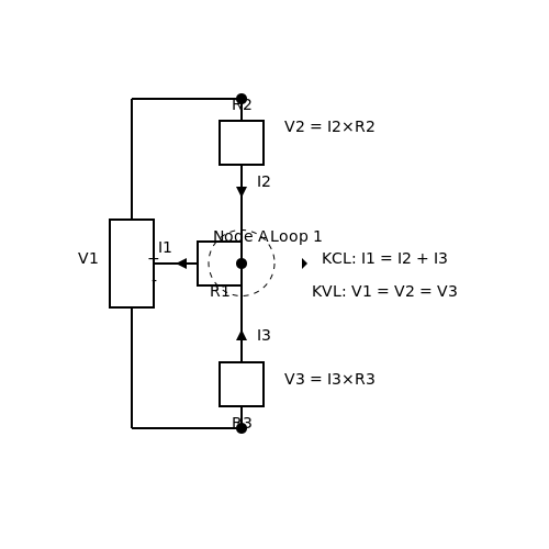
Kirchhoff's Current Law (KCL) and Kirchhoff's Voltage Law (KVL) form the foundation of circuit analysis, providing systematic methods to solve complex networks. These laws are direct consequences of charge conservation and energy conservation, respectively.
Kirchhoff's Current Law (KCL)
KCL states that the algebraic sum of currents entering any node in a circuit must equal zero:
where Ik represents the current flowing into or out of the node. Currents entering the node are conventionally considered positive, while those leaving are negative. This law enforces charge conservation at every junction.
Kirchhoff's Voltage Law (KVL)
KVL asserts that the sum of potential differences around any closed loop in a circuit must equal zero:
where Vk denotes the voltage across each component in the loop. The law reflects energy conservation, as the work done per unit charge around a closed path must balance.
Practical Applications
These laws find extensive use in:
- Circuit analysis - Solving for unknown currents and voltages in complex networks
- Power distribution systems - Balancing loads and ensuring proper current flow
- Electronic design - Verifying circuit behavior before implementation
Advanced Analysis Techniques
For networks with multiple loops and nodes, systematic approaches using Kirchhoff's laws include:
Mesh Current Method
This technique applies KVL to independent loops (meshes) in planar circuits. The procedure involves:
- Assigning clockwise or counterclockwise mesh currents
- Writing KVL equations for each mesh
- Solving the resulting system of equations
Nodal Analysis
This method uses KCL at principal nodes (excluding the reference node). The steps include:
- Selecting a reference node (typically ground)
- Applying KCL at each remaining independent node
- Expressing currents in terms of node voltages
- Solving the resulting matrix equation
Matrix Formulation
For large networks, the system of equations from Kirchhoff's laws can be expressed in matrix form:
where A is the coefficient matrix, x contains the unknown currents or voltages, and b represents the source terms. This formulation enables efficient computational solutions.
Nonlinear and Time-Varying Circuits
While Kirchhoff's laws remain valid for nonlinear components (diodes, transistors) and time-varying circuits, their application requires:
- Linearization techniques for nonlinear elements
- Differential equations for reactive components
- Numerical methods for complex systems
Experimental Verification
Practical validation of Kirchhoff's laws involves:
- Precision current measurements at nodes (KCL verification)
- Accurate voltage measurements around loops (KVL verification)
- Accounting for measurement errors and parasitic effects
Limitations and Considerations
While universally applicable, practical implementations must consider:
- High-frequency effects where lumped element models break down
- Distributed parameter systems (transmission lines)
- Quantum mechanical regimes where classical circuit theory fails
1.3 Superposition Theorem
The Superposition Theorem is a fundamental principle in linear network analysis, enabling the decomposition of complex circuits into simpler, single-source subproblems. It states that the total response (voltage or current) in any linear bilateral network with multiple independent sources is the algebraic sum of the individual responses caused by each source acting alone, while all other independent sources are turned off.
Mathematical Foundation
For a network with N independent sources, the superposition principle can be expressed as:
where Vk or Ik represents the contribution from the k-th source when all other independent sources are deactivated:
- Voltage sources are replaced with short circuits (V = 0).
- Current sources are replaced with open circuits (I = 0).
Step-by-Step Application
- Isolate each independent source sequentially, turning off all others.
- Analyze the circuit for the remaining active source using standard techniques (Ohm’s Law, nodal/mesh analysis).
- Sum the contributions algebraically, accounting for direction (polarity for voltages, flow direction for currents).
Practical Example: Dual-Source Circuit
Consider a resistive network with a voltage source V1 and current source I2:
Step 1: Deactivate I2 (open circuit) and solve for V1's contribution to current IR1:
Step 2: Deactivate V1 (short circuit) and solve for I2's contribution:
Total current: Superimpose the results:
Key Limitations
- Nonlinear systems: Applies only to linear networks (Ohm’s Law must hold).
- Dependent sources: Must remain active during analysis; only independent sources are deactivated.
- Power calculations: Superposition cannot be used directly for power, as it is quadratic in V or I.
Advanced Applications
In small-signal analysis of transistor amplifiers, superposition separates DC bias and AC signal analysis. The theorem also underpins noise analysis, where individual noise sources are evaluated independently and combined via root-mean-square summation.
1.4 Thevenin's Theorem
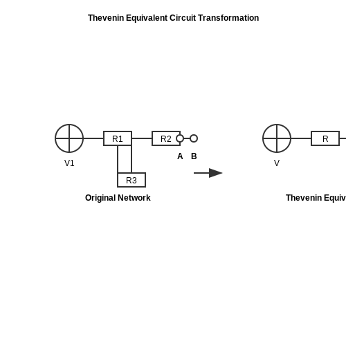
Thevenin's Theorem simplifies the analysis of complex linear networks by reducing them to an equivalent circuit consisting of a single voltage source and a series resistance. This theorem is particularly useful when analyzing the behavior of a network at a specific pair of terminals.
Mathematical Formulation
For any linear two-terminal network with independent and dependent sources, Thevenin's Theorem states that the network can be replaced by an equivalent circuit comprising:
- A voltage source VTh (Thevenin voltage), equal to the open-circuit voltage across the terminals.
- A resistance RTh (Thevenin resistance), equal to the equivalent resistance seen from the terminals with all independent sources deactivated (voltage sources shorted, current sources opened).
where VOC is the open-circuit voltage and ISC is the short-circuit current.
Step-by-Step Derivation
1. Calculating Thevenin Voltage (VTh)
To determine VTh, follow these steps:
- Remove the load resistor (if any) connected across the terminals of interest.
- Compute the open-circuit voltage (VOC) across these terminals using standard circuit analysis techniques (e.g., nodal or mesh analysis).
2. Calculating Thevenin Resistance (RTh)
The Thevenin resistance can be found using one of the following methods:
- Deactivation Method: Deactivate all independent sources (replace voltage sources with short circuits and current sources with open circuits). Compute the equivalent resistance seen from the terminals.
- Test Source Method: Apply a test voltage Vtest across the terminals and measure the resulting current Itest. Then, RTh = Vtest / Itest.
- Short-Circuit Current Method: Short the terminals and compute the short-circuit current ISC. Then, RTh = VOC / ISC.
Practical Example
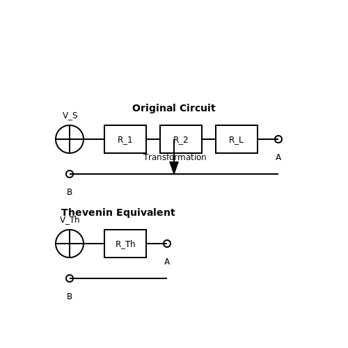
Consider a network with a voltage source VS = 10V, resistors R1 = 4Ω, R2 = 6Ω, and a load resistor RL = 5Ω connected across terminals A and B.
- Find VTh: Disconnect RL and compute VOC across A and B. Using voltage division:
$$ V_{Th} = V_{OC} = V_S \cdot \frac{R_2}{R_1 + R_2} = 10 \cdot \frac{6}{4 + 6} = 6V $$
- Find RTh: Deactivate VS (short circuit) and compute the equivalent resistance:
$$ R_{Th} = R_1 \parallel R_2 = \frac{4 \times 6}{4 + 6} = 2.4Ω $$
The Thevenin equivalent circuit is a 6V source in series with a 2.4Ω resistor. The load current can then be calculated as:
Applications in Real-World Circuits
Thevenin's Theorem is widely used in:
- Power Systems: Simplifying grid analysis for fault current calculations.
- Amplifier Design: Modeling input and output impedances of transistor circuits.
- Sensor Networks: Determining the equivalent source resistance for maximum power transfer.
For dependent sources, the same principles apply, but RTh must be computed using the test source method due to the presence of controlled quantities.
Limitations
Thevenin's Theorem is strictly applicable to linear networks. Nonlinear elements (e.g., diodes, transistors in saturation) require alternative modeling techniques such as small-signal approximation.
1.5 Norton's Theorem
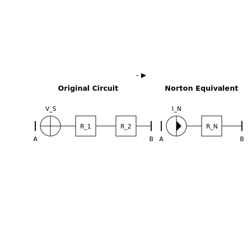
Norton's Theorem states that any linear two-terminal network containing independent and dependent sources can be replaced by an equivalent circuit consisting of a current source IN in parallel with a resistor RN. The theorem is a dual of Thévenin's Theorem, where voltage sources and series resistances are replaced by current sources and parallel conductances.
Mathematical Derivation
To derive Norton's equivalent circuit, follow these steps:
- Find the Norton current (IN): This is the short-circuit current flowing through the terminals of the network when the load is removed.
- Find the Norton resistance (RN): This is the equivalent resistance seen from the terminals when all independent sources are turned off (voltage sources shorted, current sources opened).
- Construct the Norton equivalent circuit: Place IN in parallel with RN.
Practical Applications
Norton's Theorem is particularly useful in:
- Power system analysis, where current sources model fault conditions.
- Transistor amplifier design, simplifying small-signal models.
- Circuit simulation, reducing complex networks for faster computation.
Example Calculation
Consider a network with a voltage source VS = 10V and resistors R1 = 2Ω, R2 = 3Ω:
- Find IN: Short the output terminals and compute the current.
- Find RN: Deactivate the source and compute the equivalent resistance.
The resulting Norton equivalent circuit is a 5A current source in parallel with a 1.2Ω resistor.
Comparison with Thévenin's Theorem
While Thévenin's Theorem uses a voltage source and series resistance, Norton's Theorem employs a current source and parallel resistance. Conversion between the two is straightforward:
Choosing between them depends on whether the circuit analysis favors current or voltage sources.
1.6 Maximum Power Transfer Theorem
The Maximum Power Transfer Theorem (MPTT) states that maximum power is transferred from a source to a load when the load resistance equals the Thévenin equivalent resistance of the source network. This principle is fundamental in designing efficient power delivery systems, particularly in RF circuits, audio amplifiers, and impedance-matching networks.
Mathematical Derivation
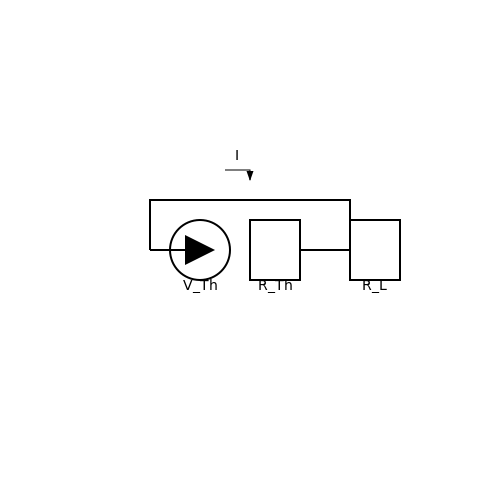
Consider a DC source network represented by its Thévenin equivalent: a voltage source $$V_{Th}$$ in series with a resistance $$R_{Th}$$. The load resistance is $$R_L$$. The power dissipated in the load is:
To find the condition for maximum power transfer, we differentiate $$P_L$$ with respect to $$R_L$$ and set the derivative to zero:
Simplifying, we obtain:
Which reduces to:
Thus, maximum power transfer occurs when the load resistance matches the Thévenin resistance of the source.
Power Efficiency Consideration
While MPTT ensures maximum power transfer, it does not guarantee maximum efficiency. The efficiency $$\eta$$ under maximum power transfer conditions is only 50%, since half the power is dissipated in the source resistance:
This trade-off is critical in applications where energy efficiency is prioritized over power transfer, such as in battery-operated systems.
AC Circuit Generalization
For AC circuits, the theorem extends to complex impedances. Maximum power transfer occurs when the load impedance $$Z_L$$ is the complex conjugate of the Thévenin impedance $$Z_{Th}$$:
This ensures that the reactive components cancel out, leaving only resistive power dissipation.
Practical Applications
- RF and Antenna Design: Impedance matching ensures maximum power transfer from transmitters to antennas.
- Audio Systems: Amplifiers and speakers are designed with matched impedances to optimize power delivery.
- Renewable Energy: Solar panels and wind turbines use MPTT-based algorithms (MPPT) to extract maximum available power.
Limitations and Misconceptions
The theorem is often misapplied in scenarios where efficiency is more critical than power transfer. Additionally, nonlinear loads or time-varying sources require dynamic impedance matching techniques beyond the static MPTT assumption.
2. Circuit Simplification Techniques
2.1 Circuit Simplification Techniques
Series and Parallel Reduction
Resistors, capacitors, and inductors in series or parallel configurations can be simplified using fundamental reduction techniques. For resistors in series, the equivalent resistance Req is the sum of individual resistances:
For parallel resistors, the equivalent conductance is additive:
These principles extend to reactive components, where impedance Z replaces resistance. For inductors in series, inductances add linearly, while parallel inductors follow the reciprocal rule. Capacitors behave inversely—series combinations use reciprocal summation, while parallel capacitances add directly.
Star-Delta (Y-Δ) Transformation
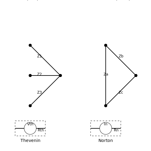
When dealing with three-terminal networks, the Y-Δ transformation allows conversion between star (Y) and delta (Δ) configurations. Given three impedances Za, Zb, Zc in a delta configuration, the equivalent star impedances are:
This transformation is particularly useful in power systems and filter design, where symmetrical networks simplify analysis.
Thevenin and Norton Equivalents
Any linear two-terminal network can be reduced to a Thevenin equivalent (a voltage source Vth in series with a resistance Rth) or a Norton equivalent (a current source In in parallel with Rth). Thevenin voltage is the open-circuit voltage, while Norton current is the short-circuit current:
These equivalents are indispensable in load analysis, maximizing power transfer, and simplifying complex networks for transient analysis.
Superposition Principle
For linear circuits with multiple independent sources, the superposition principle states that the total response is the sum of individual responses due to each source acting alone. To apply:
- Deactivate all sources except one (replace voltage sources with shorts, current sources with opens).
- Solve for the desired voltage or current.
- Repeat for each source and sum the contributions algebraically.
This method is particularly effective in analyzing circuits with mixed AC and DC sources or multiple frequency components.
Source Transformation
A voltage source V in series with a resistance R can be converted to an equivalent current source I = V/R in parallel with R, and vice versa. This technique simplifies nodal or mesh analysis by reducing the number of variables.
Practical applications include simplifying amplifier biasing networks and power supply designs.
Symmetry Exploitation
In symmetrical circuits, identical branches can be analyzed once, with results mirrored across the symmetry axis. For example, a Wheatstone bridge in balance satisfies:
When balanced, the central branch carries no current, allowing its removal or short-circuiting for simplification. Symmetry is frequently leveraged in differential amplifiers and transmission line analysis.
Dimensional Reduction via Matrix Methods
For large-scale networks, graph theory and matrix algebra provide systematic simplification. The incidence matrix A relates nodes to branches, while the loop matrix B defines independent meshes. Kirchhoff’s laws translate to:
Combined with Ohm’s law, these yield compact representations solvable via Gaussian elimination or sparse matrix techniques, essential in computational circuit analysis tools like SPICE.
2.2 Analyzing Complex Networks
Nodal Analysis with Supernodes
When analyzing circuits with voltage sources between non-reference nodes, standard nodal analysis requires modification. A supernode forms when a voltage source connects two non-reference nodes, creating a constrained system. The key steps are:
- Enclose the voltage source and its two nodes within a single supernode boundary.
- Write a KCL equation for the entire supernode, treating currents entering/leaving the boundary.
- Add the voltage source's constraint equation relating the two nodal voltages.
For a circuit with supernode between nodes V1 and V2 with source voltage Vs:
Mesh Analysis with Current Sources
Current sources in parallel with components create supermeshes - regions where standard mesh analysis fails. The solution involves:
- Removing the current source from the circuit temporarily
- Defining a larger mesh that encompasses both original meshes adjacent to the current source
- Writing KVL for the supermesh
- Adding the current source's constraint equation
For two meshes i1 and i2 sharing current source Is:
Network Reduction Techniques
For large networks, systematic reduction methods improve computational efficiency:
| Method | Application | Complexity Reduction |
|---|---|---|
| Y-Δ Transformation | 3-terminal networks | O(n2) → O(n) |
| Source Transformation | Mixed source networks | Eliminates equations |
| Equivalent Resistance | Series/parallel sections | Node elimination |
Y-Δ Transformation Equations
Conversion between wye (Y) and delta (Δ) configurations:
Computer-Aided Network Analysis
Modern circuit simulation tools use modified nodal analysis (MNA) which systematically handles:
- Nonlinear components through Newton-Raphson iteration
- Frequency-domain analysis via complex impedance matrices
- Time-domain simulation using numerical integration methods
The MNA matrix formulation for a linear network:
Where G contains conductances, B/C describe source connections, and D represents source constraints.
2.3 Designing Efficient Power Systems
Power Transfer Efficiency and Maximum Power Transfer Theorem
The Maximum Power Transfer Theorem (MPTT) states that maximum power is delivered to a load when its impedance equals the complex conjugate of the source impedance. For a DC system with source resistance RS and load resistance RL, this reduces to RL = RS. The power delivered to the load is:
Differentiating PL with respect to RL and setting the derivative to zero confirms the maximum power condition. However, this theorem assumes 50% efficiency at maximum power transfer, which is often impractical in high-efficiency power systems. Instead, engineers optimize for a balance between power delivery and efficiency by selecting RL ≫ RS.
Superposition Theorem in Multi-Source Networks
In power systems with multiple sources (e.g., grid-tied inverters, hybrid generators), the Superposition Theorem simplifies analysis by evaluating each source independently. For a network with N voltage sources, the total current through a branch is:
where Ik is the current contribution from the k-th source when all other sources are deactivated (voltage sources short-circuited, current sources open-circuited). This method is critical for fault analysis and load sharing in microgrids.
Thévenin Equivalent for Grid Stability
Reducing complex power networks to a Thévenin equivalent (voltage source VTh in series with impedance ZTh) enables rapid stability assessment. For a transmission line modeled as a π-network, the equivalent impedance is:
where Z11, Z12, and Z22 are the line’s impedance matrix elements. This simplification aids in calculating fault currents and designing protective relaying schemes.
Norton’s Theorem for Parallel Source Integration
Distributed energy resources (DERs) like solar arrays often behave as current sources. The Norton equivalent (current source IN in parallel with admittance YN) simplifies parallel source integration. The combined Norton current for M parallel DERs is:
while the equivalent admittance is the sum of individual admittances. This approach is foundational for inverter-dominated grids.
Reciprocity Theorem for Sensor Placement
The Reciprocity Theorem validates that power transfer between two nodes is unchanged if source and measurement locations are swapped. For a grid with impedance matrix Z, the theorem ensures:
This principle optimizes phasor measurement unit (PMU) placement for observability in smart grids.
Practical Case Study: Microgrid Design
A 10 kW microgrid with diesel generators (ZTh = 0.2 + j0.5 Ω) and battery storage (YN = 0.1 – j0.3 S) demonstrates these theorems. Using Thévenin-Norton conversions, the system’s peak efficiency (94%) occurs at Zload = 0.22 – j0.48 Ω, derived via:
2.4 Troubleshooting Electrical Circuits
Diagnosing Faults Using Network Theorems
When an electrical circuit malfunctions, systematic troubleshooting requires applying network theorems to isolate faulty components. Thevenin’s and Norton’s theorems simplify complex networks into equivalent circuits, making it easier to measure deviations from expected behavior. For instance, if a resistive branch draws abnormal current, replacing the rest of the circuit with its Thevenin equivalent allows direct computation of the expected current:
If the measured current differs significantly, the fault likely lies in either Rload or the upstream network. Superposition theorem further aids in isolating AC/DC faults by analyzing the circuit’s response to individual sources.
Practical Techniques for Open and Short Circuits
Common failures include open circuits (infinite resistance) and short circuits (near-zero resistance). To locate these:
- Voltage measurements: An open component shows full supply voltage across its terminals, while a short exhibits near-zero voltage.
- Current measurements: Use Norton’s equivalent to predict branch currents; discrepancies indicate faults.
- Resistance checks: Power off the circuit and measure resistance across suspected components.
Case Study: Thevenin’s Theorem in Fault Isolation
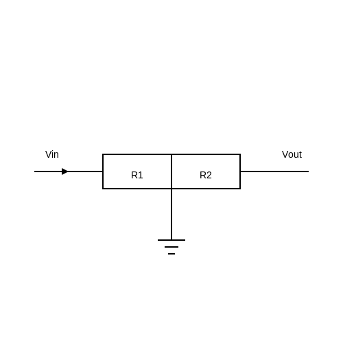
Consider a voltage divider circuit where the output voltage drops unexpectedly. By deriving the Thevenin equivalent (VTh = open-circuit voltage, RTh = equivalent resistance), the expected output under load is:
A deviation suggests either Rload is faulty or the Thevenin parameters (indicating upstream resistor degradation).
Advanced Tools: Nodal and Mesh Analysis
For circuits with multiple unknowns, nodal analysis (Kirchhoff’s Current Law) or mesh analysis (Kirchhoff’s Voltage Law) provides a systematic approach. For example, nodal analysis for a circuit with n nodes yields:
where Gjk is the conductance matrix and Iext,j is the external current injection. Discrepancies between calculated and measured node voltages reveal faulty components.
Real-World Considerations
In practice, parasitic capacitances, inductances, and non-ideal instrument resistances (e.g., multimeter loading) affect measurements. Always:
- Account for meter impedance when measuring high-resistance circuits.
- Use frequency-domain analysis (phasors) for AC circuits with reactive components.
- Validate assumptions (e.g., linearity) when applying superposition.
The above diagram illustrates a voltage divider where R2’s failure would directly impact Vout.
3. Network Theorems in AC Circuits
Network Theorems in AC Circuits
Superposition Theorem in AC Circuits
The superposition theorem remains valid in AC circuits, provided the system is linear. For a circuit with multiple AC sources, the total response is the phasor sum of individual responses caused by each source acting alone. Consider a circuit with two voltage sources V1(ω) and V2(ω). The current through any element is:
where I1 is the current due to V1 alone (with V2 replaced by its internal impedance), and I2 is the current due to V2 alone. This principle is particularly useful in analyzing circuits with multiple frequencies, where each frequency component can be treated separately.
Thevenin's and Norton's Theorems for AC Networks
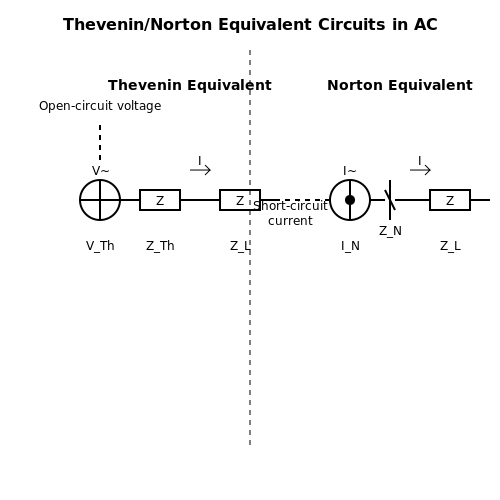
In AC circuits, Thevenin's theorem states that any linear two-terminal network can be replaced by an equivalent circuit consisting of a voltage source VTh in series with an impedance ZTh. Thevenin voltage is the open-circuit voltage across the terminals, while Thevenin impedance is the equivalent impedance seen from the terminals with all independent sources deactivated (voltage sources shorted, current sources opened).
Norton's equivalent replaces the network with a current source IN in parallel with an impedance ZN, where IN is the short-circuit current and ZN = ZTh. These theorems are invaluable in simplifying complex AC networks for power transfer analysis.
Maximum Power Transfer Theorem in AC Circuits
For maximum power transfer in an AC circuit, the load impedance ZL must be the complex conjugate of the Thevenin impedance ZTh of the source network:
This condition ensures that the reactive components cancel out, and the resistive part of the load matches the source resistance. The maximum power delivered is then:
This principle is critical in RF and audio amplifier design, where impedance matching optimizes power efficiency.
Reciprocity Theorem in AC Systems
The reciprocity theorem holds for linear, bilateral AC networks. It states that the ratio of the voltage (or current) response in one branch to the current (or voltage) source in another branch remains unchanged if the positions of the source and response are interchanged. Mathematically, for a voltage source V and current response I:
This theorem is particularly useful in antenna theory and filter design, where symmetry in network response is exploited.
Millman's Theorem for AC Voltage Sources
Millman's theorem extends to AC circuits with multiple parallel voltage sources. The equivalent voltage Veq is given by the phasor sum of individual source voltages weighted by their admittances:
where Yk = 1/Zk is the admittance of each branch. This simplifies the analysis of unbalanced polyphase systems and parallel-connected AC generators.
Compensation Theorem for AC Networks
The compensation theorem allows analyzing the effect of impedance changes in an AC network. If an impedance Z in a branch changes by ΔZ, the resulting change in current ΔI can be modeled by introducing a compensating voltage source Vc = I · ΔZ in series with the modified branch, where I is the original current. This is useful in sensitivity analysis and fault tolerance studies.
Non-linear Circuit Analysis
Fundamentals of Non-linear Elements
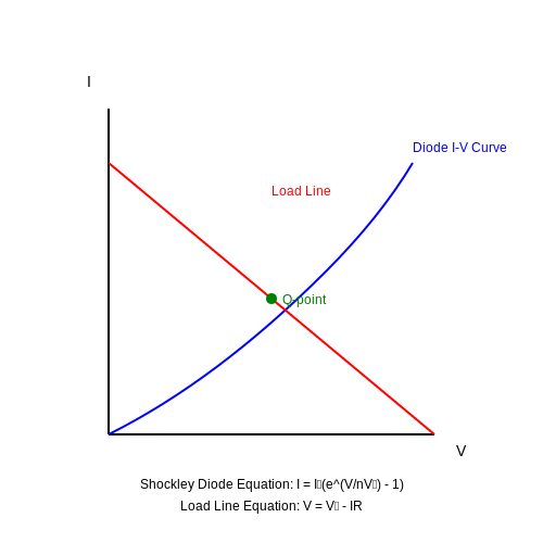
Non-linear circuit elements, such as diodes, transistors, and varistors, exhibit a voltage-current relationship that does not follow Ohm's Law. Unlike linear resistors, where V = IR holds, non-linear devices obey more complex governing equations. For instance, the Shockley diode equation describes the current I through a diode as:
where IS is the reverse saturation current, V is the voltage across the diode, n is the ideality factor, and VT is the thermal voltage (≈25.85 mV at 300 K). This exponential relationship complicates analytical solutions, necessitating numerical or graphical methods.
Graphical Analysis: Load Line Method
For simple non-linear circuits, the load line technique provides an intuitive graphical solution. Consider a diode-resistor circuit powered by a voltage source VS:
Plotting the diode's I-V curve alongside the linear load line (derived from the equation above) yields the operating point at their intersection. This method is particularly useful for power electronics design, where biasing conditions must be precisely determined.
Small-Signal Approximation
When non-linear devices operate with a small AC signal superimposed on a DC bias, linearization around the operating point simplifies analysis. The Taylor series expansion truncates to first-order terms, yielding equivalent small-signal parameters:
where rd is the dynamic resistance of the diode. This approach is foundational in amplifier design, where transistors are biased in their active region and small variations are analyzed using hybrid-π models.
Iterative Numerical Methods
For complex non-linear networks, Newton-Raphson iteration provides a computationally efficient solution. The algorithm linearizes the system at each step using the Jacobian matrix J of partial derivatives:
SPICE simulators employ this method with adaptive step-sizing to solve nodal equations. Convergence criteria typically require residual currents below 1 nA or voltage mismatches under 1 μV for precision circuits.
Piecewise Linear Modeling
Non-linear characteristics are often approximated by connected linear segments. A diode, for example, can be modeled as:
- An open circuit for V < Vγ (cut-in voltage)
- A fixed voltage source Vγ in series with resistance rd for V ≥ Vγ
This simplification enables rapid hand calculations in power supply design and clipping circuit analysis while maintaining reasonable accuracy.
Harmonic Balance for RF Circuits
High-frequency non-linear systems, such as mixers and oscillators, require harmonic balance analysis. The method solves for steady-state conditions by balancing frequency-domain currents:
Commercial tools like Keysight ADS use this technique to predict intermodulation distortion and spectral regrowth in communication systems, where non-linearities generate unwanted harmonics.
3.3 Real-world Engineering Problems
Power Distribution Networks
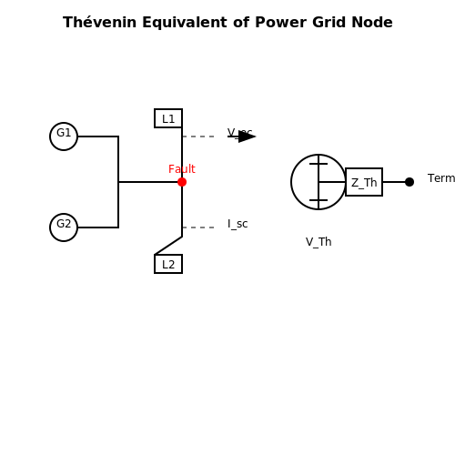
In large-scale power grids, Thévenin’s theorem simplifies complex transmission networks into equivalent circuits for fault analysis. Consider a grid with distributed generators and loads. The Thévenin equivalent voltage VTh and impedance ZTh at a node are derived by:
This model predicts voltage sags during faults, enabling protective relay coordination. For example, a 10 kV distribution line with ZTh = 0.5 + j1.2 Ω and a fault current of 2 kA implies:
Active Filter Design
Superposition theorem aids in analyzing harmonic mitigation circuits. In a three-phase active power filter, each harmonic component (e.g., 5th, 7th) is treated as an independent source. The total compensating current Ic is the sum of individual harmonic contributions:
Practical implementations use Fast Fourier Transform (FFT) to decompose load currents, with Norton equivalents representing each harmonic’s current source and parallel impedance.
Wireless Communication Systems
Maximum Power Transfer theorem optimizes antenna matching networks. For a receiver with input impedance Zin = R + jX, the conjugate matching condition (ZL = Zin*) ensures maximum power transfer. The power delivered to the load is:
In 5G systems, this principle minimizes reflections at mmWave frequencies, where a 1 dB mismatch can degrade SNR by 20%.
Integrated Circuit Testing
Norton’s theorem models defective IC pins as current sources. A short-circuited pin injects a fault current IN, while the Norton resistance RN represents the defect’s impedance. Automated test equipment (ATE) measures these parameters to localize defects:
For a CMOS inverter with a bridging fault, RN typically ranges from 10 Ω (metal short) to 1 kΩ (gate oxide leakage).
Renewable Energy Integration
Millman’s theorem aggregates distributed renewable sources into a single equivalent voltage. For n solar inverters with outputs V1...Vn and internal resistances R1...Rn, the equivalent grid-tie voltage is:
This simplifies stability analysis for microgrids with 30+ inverters, reducing computational overhead by 75% compared to full nodal analysis.
Case Study: DC Railway Electrification
Reciprocity theorem validates voltage drop calculations in 750 V DC traction systems. By interchanging the positions of a train load (say, 500 A at 1 km) and a monitoring probe, the theorem confirms consistency:
Field measurements in the London Underground showed < 2% deviation from theoretical predictions, validating the model’s accuracy for infrastructure upgrades.
4. Recommended Textbooks
4.1 Recommended Textbooks
- Chapter 4 Network Theorems | PDF | Electrical Network | Electronic ... — The document discusses various network theorems including superposition, source transformation, Thevenin's theorem, Norton's theorem, and maximum power transfer. It provides examples and solutions for applying each theorem to example circuits. Tutorial questions at the end provide additional practice problems applying the network theorems.
- Electrical Network Theorems and Their Applications — Network theorems are tools to convert complicated electric networks into simpler equivalents. Important network theorems, their proof and applications in different situations are discussed in this chapter.
- PDF "Modular Electronics Learning (ModEL) project" — Similarly, network theorems are proven tools useful for quickly and easily analyzing complex electrical networks without being limited to fundamental rules such as Ohm's Law and Kirchhoff's Laws. Th ́evenin's and Norton's Theorems are two such network theorems, and they find frequent application in electronic circuit analysis.
- PDF Kirchhoff's laws and their applications in solving electrical network ... — 2.1 Ohm's law, resistances in series and parallel 2.2 Kirchhoff's laws and their applications in solving electrical network problems 2.3 Network theorems such as Thevenin's theorem, superposition theorem Maximum power and transfer theorem and Norton's theorem
- PDF Network Theorems - Springer — These cumbersome mathematical analyses can be simplified by using advanced techniques known as network or circuit theorems. These include linearity property, superposition theorem, Thevenin's theorem, Norton's theorem and maximum power transfer theorem. Here, most of these theorems will be discussed with independent and dependent sources.
- PDF 1 Elementary electrical circuit analysis - Elsevier — The fundamental tools for electrical circuit analysis Kirchhoff's laws are discussed in section 1.4. Then, three very important electrical network the-orems; Th ́evenin's theorem, Norton's theorem and the superposition theorem are presented. The unit system used in this book is the International System of Units (SI) [1].
- Electrical Circuit Analysis & Network Theory Textbook — Textbook covering electrical circuit analysis, network theorems, Laplace transforms, Fourier analysis, and two-port networks for EE students.
- Electrical and Electronic Technology Textbook — Comprehensive textbook on electrical and electronic technology for engineering students. Covers electrical principles, electronics, power, and measurements.
- PDF DC Electrical Circuit Analysis - dissidents — nt, energy, power and voltage. Subsequent chapters introduce resistance, series circuits, parallel circuit and series-parallel circuits. The text continues with chapters covering network theorems, more advanced techniques such as nodal and mesh analysis, and finally finishes with introductions to capacitors, i
4.2 Research Papers and Articles
- Chapter 4 Network Theorems | PDF | Electrical Network | Electronic ... — 4 NETWORK THEOREMS. 4.1 Superposition 4.2 Source Transformation 4.3 Thevenin's Theorem 4.4 Norton's Theorem 4.5 Maximum Power Transfer. 4.1 SUPERPOSITION. The superposition theorem states that the voltage across (or current through) an element in a circuit is the algebraic sum of the voltages across (or currents through) that elements due to each independent source acting alone.
- (PDF) DC NETWORK THEOREMS - Academia.edu — Academia.edu is a platform for academics to share research papers. DC NETWORK THEOREMS ... The equivalent resitance of the two parallel paths across point a is 3 || (4 +2) =2Q Now, applying KVL to the closed loop, we get 24 —-v —2v -2i = 0. ... Norton's theorem replaces the network by an equivalent constant-current source and a parallel ...
- PDF Kirchhoff's laws and their applications in solving electrical network ... — 2.2 Kirchhoff's laws and their applications in solving electrical network problems 2.3 Network theorems such as Thevenin's theorem, superposition theorem Maximum power and transfer theorem and Norton's theorem 3. Batteries (15 Periods) 3.1 Basic idea about primary and secondary cells
- Electric Network Analysis - an overview | ScienceDirect Topics — 4 Detailed review and analysis. Network analysis is an emerging trend in the current era due to its large variety of applications in different fields (Galaskiewicz and Wasserman, 1993).This analysis can be done in various networks like; social networks, road networks, biological networks, information networks, etc. (Wasserman, 1994, Scott, 1988, Borgatti et al., 2009).
- Electrical Network Theorems and Their Applications — Network theorems are tools to convert complicated electric networks into simpler equivalents. Important network theorems, their proof and applications in different situations are discussed in this chapter. ... A planner circuit is a circuit that may be drawn on a piece of paper, i.e. circuit elements are all arranged in only two dimensions ...
- PDF Chapter 4 Network Theorems - Springer — Network Theorems 4.1 Introduction Fundamental electrical laws and the associated methods of analysis, which have been discussed in the previous chapters, need tedious mathematical manipulation. These cumbersome mathematical analyses can be simplified by using advanced techniques known as network or circuit theorems. These include linearity ...
- Network Theorems - SpringerLink — These cumbersome mathematical analyses can be simplified by using advanced techniques known as network or circuit theorems. These include linearity property, superposition theorem, Thevenin's theorem, Norton's theorem and maximum power transfer theorem. ... {1.5}{1.5 + 4} = 2.73\,{\text{A}}$$ (4.39) Finally, the current in the \(4\,{\Omega ...
- (PDF) Hand Book of Electronics - ResearchGate — PDF | On Jan 1, 2010, D.K. Kaushik published Hand Book of Electronics | Find, read and cite all the research you need on ResearchGate
- PDF NETWORK ANALYSIS & SYNTHESIS - Veer Surendra Sai University of Technology — IMPEDANCE FUNCTIONS AND NETWORK THEOREMS: The Concept of Complex Frequency, Transform Impedance and Transform Circuit, Series and parallel Combination of ... TESTING DRIVING-POINT FUNCTIONS: An application of the Maximum Modulus Theorem, Properties of Hurwitz Polynomials, The Computation of Residues, Even and Odd functions, Sturm's Theorem ...
- PDF Network Theory [SD] - Netaji Subhash Engineering College — Basics of Circuit Theory & Network Theorems 1.1.5: Unilateral Element Conduction of current in one direction is termed as unilateral (example: Diode, Transistor) element. Fig. 1.2 Unilateral element 1.1.6: Meaning of Response An application of input signal to the system will produce an output signal, the behavior of output
4.3 Online Resources and Tutorials
- NETWORK THEOREMS - Chapter four Network Theorems - 1Library — Now that the network has been reduced to a simple series circuit the total effective resistance is R=R1+R2+Re=8 +6 +5.33 =19.33Ω I V R. = = 87 = 19 33 4.5 A R R R R R e= + = × + = . 3 4 3 4 16 8 16 8 5 33Ω V I 1 1 22 2 = =11Ω Fig. 4.3 Circuit diagram for Example 4.3 CHAPTER 4 NETWORK THEOREMS 65
- Chapter 4 Network Theorems | PDF | Electrical Network | Electronic ... — 4 NETWORK THEOREMS. 4.1 Superposition 4.2 Source Transformation 4.3 Thevenin's Theorem 4.4 Norton's Theorem 4.5 Maximum Power Transfer. 4.1 SUPERPOSITION. The superposition theorem states that the voltage across (or current through) an element in a circuit is the algebraic sum of the voltages across (or currents through) that elements due to each independent source acting alone.
- Electrical Network Theorems and Their Applications — Electrical/electronic network, branch, node, loop and mesh. ... Fundamental network theorems and their applications will be discussed in the following. 1.4.1 Superposition Theorem. The superposition theorem is the most fundamental theorem that is applicable to both DC and AC networks. The theorem applies to those networks which have many ...
- Network analysis 3rd sem - Kiran Kumar V UNIT 4 : NETWORK THEOREMS II ... — The statement of this theorem is slightly different for D. circuits and A circuits. 4.3. Statement For D. Circuits: Maximum power will be transferred to the load by the. network when the load resistance is equal to the internal resistance (=R TH) of the. network. Consider the Thevinin's equivalent circuit of a given network as in figure 4(a ...
- PDF Chapter 4 Network Theorems - Springer — Network Theorems 4.1 Introduction Fundamental electrical laws and the associated methods of analysis, which have been discussed in the previous chapters, need tedious mathematical manipulation. These cumbersome mathematical analyses can be simplified by using advanced techniques known as network or circuit theorems. These include linearity ...
- Industrial Electronics N4 Lecturer Guide Extract - Calaméo — 1 Module Network theorems Module outline 5 Unit 1.1 Kirchhoff's laws Unit 1.2 Superposition theorem d Unit 1.3 Thevenin's theorem an Unit 1.4 Norton's theorem Unit 1.5 Maximum power transfer theorem using Nodal analysis and Thevenin's equivalent circuits. 2 1, Resources s es When teaching this module you can use the following teaching ...
- EE Lecture 4 - Superposition - Thevenan - Norton — The document introduces four network theorems: the superposition theorem, Thévenin's theorem, Norton's theorem, and the maximum power transfer theorem. It provides detailed explanations and examples of applying the superposition theorem, Thévenin's theorem, and Norton's theorem to determine unknown currents and voltages in circuits by reducing networks to their equivalent representations ...
- (PDF) EEEB113 - Chapter 4 - Academia.edu — 4 5/25/2011 4.3 superposition theorem (4) $ # 1. Turn off all independent sources except one source. Find the output (voltage or current) due to that active source using " or ! analysis.
- PPT Topic 4 Network Theorem - repository.unikom.ac.id — CIRCUIT THEORY TUTORIAL 2 - Topic 4: Network Theorem Wei Wen Shyang EBEC3103 Circuit Theory Jan 2005
- PDF School of Electrical and Electronics Department of Electrical and ... — across their terminals. This theorem is valid only for linear systems. This theorem can be better understood with a numerical example. Consider the circuit which contains two sources as shown in Fig. 1. Now let us find the current passing through the 3 V resistors in the circuit. According to the superposition theorem, the current I 2