Definition and Components of an RC Circuit

An RC circuit consists of two fundamental passive components: a resistor (R) and a capacitor (C), connected either in series or parallel. The behavior of the circuit is governed by the interaction between these components, characterized by the time constant τ = RC, which determines the rate of charging or discharging.

Resistor (R)

The resistor imposes a linear voltage-current relationship defined by Ohm’s Law:

where V_R(t) is the instantaneous voltage across the resistor, and I(t) is the current through it. In an RC circuit, the resistor controls the rate of energy dissipation and the transient response.

Capacitor (C)

The capacitor stores energy in an electric field, with its voltage-current relationship governed by:

where V_C(t) is the voltage across the capacitor. Unlike a resistor, a capacitor’s current depends on the rate of change of voltage, leading to exponential charging/discharging behavior in RC circuits.

Time Constant (τ)

The time constant τ = RC quantifies how quickly the circuit responds to changes:

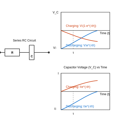
• For charging: V_C(t) = V_0 (1 - e^{-t/τ})
• For discharging: V_C(t) = V_0 e^{-t/τ}

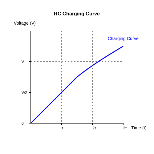
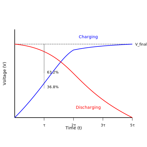
At t = τ, the capacitor reaches ~63% of its final voltage during charging or decays to ~37% during discharging.

Practical Applications

RC circuits are foundational in:

• Signal filtering: High-pass and low-pass filters exploit frequency-dependent impedance.
• Timing circuits: Used in oscillators and pulse generators due to predictable transient responses.
• Noise suppression: Bypass capacitors stabilize power supplies by shunting high-frequency noise to ground.

1.2 Time Constant (τ) and Its Significance

The time constant, denoted by τ, is a fundamental parameter in RC circuits that quantifies the rate at which the circuit responds to changes in voltage or current. It is defined as the product of the resistance R and the capacitance C:

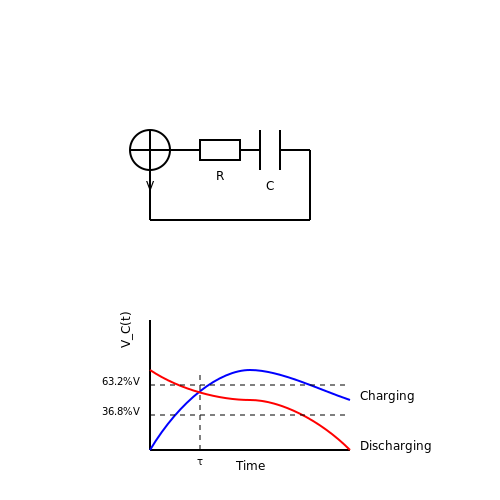
Physically, τ represents the time required for the voltage across the capacitor to reach approximately 63.2% of its final value when charging, or to decay to 36.8% of its initial value when discharging. This behavior arises from the exponential nature of the charging and discharging processes in an RC circuit.

Mathematical Derivation of the Time Constant

Consider a simple RC circuit with a voltage source V, resistor R, and capacitor C. The charging process of the capacitor is governed by Kirchhoff's voltage law:

Since current i is the time derivative of charge q, we can rewrite the equation as:

Rearranging and solving this first-order differential equation yields:

The voltage across the capacitor V_C(t) is then:

At t = τ = RC, the voltage reaches:

Significance of the Time Constant

The time constant τ is crucial for several reasons:

• Circuit Response Speed: A smaller τ indicates a faster response, while a larger τ implies slower dynamics.
• Filter Design: In RC filters, τ determines the cutoff frequency f_c:

• Pulse Shaping: In digital circuits, τ affects rise and fall times, influencing signal integrity.
• Energy Storage and Dissipation: The time constant governs how quickly energy is stored in or released from the capacitor.

Practical Applications

The concept of the time constant is applied in various real-world scenarios:

• Oscilloscope Probes: Compensation adjustments rely on matching the probe's τ to the oscilloscope's input capacitance.
• Timing Circuits: RC networks are used in monostable and astable multivibrators to generate precise delays.
• Biological Systems: The membrane time constant in neurons determines how quickly they respond to stimuli.

For a step input, the transient response settles to within 1% of the final value after approximately 5τ, a rule of thumb frequently used in circuit design.

1.3 Charging and Discharging Processes

Transient Response of an RC Circuit

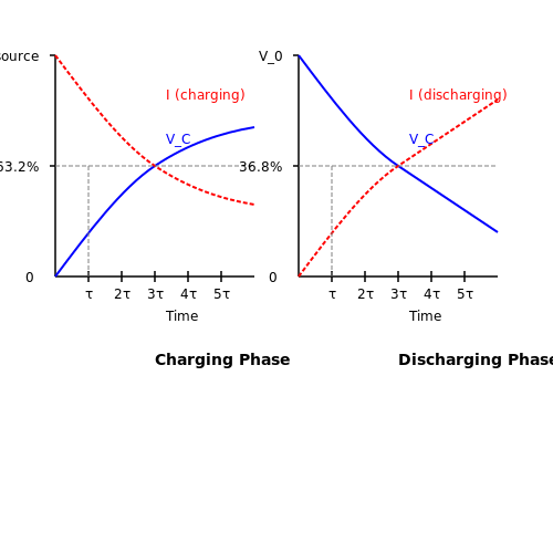
When a DC voltage source is connected to a series RC circuit, the capacitor does not charge instantaneously. Instead, the voltage across the capacitor V_C(t) and the current through the resistor I(t) follow exponential functions governed by the time constant τ = RC. The charging process is described by Kirchhoff’s voltage law:

Since V_R(t) = I(t)R and I(t) = C \frac{dV_C(t)}{dt}, the differential equation for the charging process becomes:

Charing Phase: Derivation of Voltage and Current

Solving this first-order linear differential equation with the initial condition V_C(0) = 0 yields:

The current through the circuit decays exponentially as:

The time constant τ determines how quickly the capacitor charges. At t = τ, the capacitor reaches approximately 63.2% of its final voltage. At t = 5τ, it is considered fully charged (99.3% of V_source).

Discharging Phase

When the voltage source is removed and the capacitor discharges through the resistor, the voltage across the capacitor follows:

where V_0 is the initial voltage on the capacitor. The discharge current is:

The negative sign indicates that the current flows in the opposite direction compared to the charging phase.

Practical Implications

The transient behavior of RC circuits is fundamental in applications such as:

• Timing circuits (e.g., oscillators, delay lines)
• Signal filtering (high-pass and low-pass RC networks)
• Power supply decoupling (smoothing voltage ripples)

In high-speed digital circuits, the RC time constant affects signal rise/fall times and must be minimized to prevent distortion. Conversely, in timing applications, precise control of τ ensures accurate pulse generation.

Energy Considerations

During charging, the energy supplied by the source is split between the capacitor and the resistor. The total energy dissipated in the resistor during charging is equal to the energy stored in the capacitor:

This energy balance holds regardless of the resistance value, illustrating that half the energy is lost as heat during charging.

Step Response of an RC Circuit

Fundamental Behavior

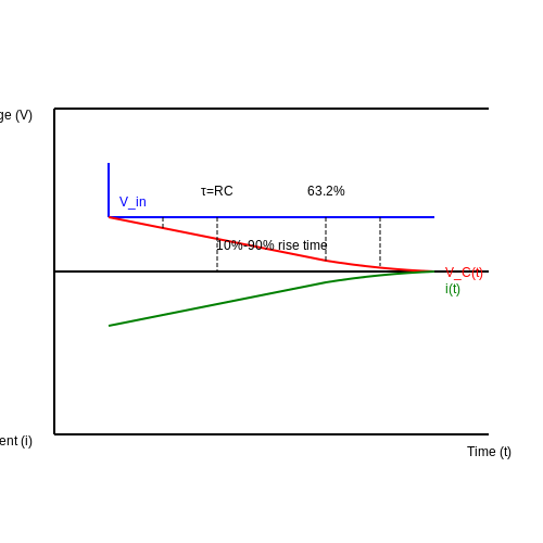
When a voltage step input is applied to a series RC circuit, the capacitor charges through the resistor, exhibiting an exponential voltage rise. The time constant τ = RC governs this transient response, representing the time required for the capacitor voltage to reach approximately 63.2% of its final value.

Mathematical Derivation

Applying Kirchhoff's voltage law to the series RC circuit with step input V_inu(t) yields:

Differentiating both sides and solving the first-order differential equation:

The complete solution consists of homogeneous and particular solutions:

Practical Characteristics

Key parameters of the step response include:

• Rise time (10% to 90%): Approximately 2.2τ
• Settling time (to within 1%): About 5τ
• Peak current: V_in/R at t=0+

Measurement Considerations

When probing RC step response in real circuits:

• Oscilloscope input capacitance (~15pF) affects high-speed measurements
• Probe compensation becomes critical for τ < 100ns
• Ground lead inductance distorts fast edges (>1MHz)

Application Example: Pulse Shaping

RC circuits intentionally modify pulse waveforms in:

• Edge detection circuits (τ << pulse width)
• High-pass filtering of digital signals
• Timing circuits where τ sets delay intervals

Non-Ideal Effects

Practical deviations from ideal behavior occur due to:

• Capacitor equivalent series resistance (ESR)
• Dielectric absorption in capacitors
• Parasitic inductance in circuit layout
• Non-zero source impedance

2.2 Natural and Forced Response

Natural Response of an RC Circuit

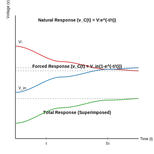
The natural response of an RC circuit describes the behavior of the circuit when it is allowed to discharge freely without any external forcing function. Consider a simple RC circuit with an initially charged capacitor C and resistor R. The voltage across the capacitor v_C(t) decays exponentially according to:

where V₀ is the initial voltage, and τ = RC is the time constant. The current i(t) through the resistor follows a similar decay:

This response is governed solely by the circuit's inherent properties (R and C) and initial conditions. The time constant τ determines how quickly the system reaches equilibrium—typically, the transient is considered negligible after 5τ.

Forced Response of an RC Circuit

The forced response arises when an external voltage or current source drives the circuit. For a DC input V_in, the capacitor charges according to:

For sinusoidal inputs, the forced response is a steady-state solution that depends on the frequency of the driving signal. The impedance of the capacitor Z_C = 1/(jωC) introduces a phase shift between voltage and current, leading to frequency-dependent behavior.

Superposition of Natural and Forced Responses

The total response of an RC circuit to a sudden change (e.g., a step input) is the sum of the natural and forced responses:

This superposition principle is fundamental to analyzing transient and steady-state behavior in linear circuits. In practical applications, such as signal filtering or power supply design, understanding this interplay ensures proper damping and stability.

Practical Implications

Time Constant Selection: In pulse shaping circuits, τ is chosen to either preserve (large τ) or differentiate (small τ) input signals. For example, an RC integrator requires τ ≫ T (signal period), while a differentiator needs τ ≪ T.

Frequency Response: For AC analysis, the cutoff frequency f_c = 1/(2πRC) defines the transition between passband and attenuation. This is critical in low-pass and high-pass filter design.

Mathematical Derivation of the Total Response

To derive the total response, solve the first-order differential equation for an RC circuit with a step input:

The homogeneous solution (natural response) is v_C,h(t) = Ae^{-t/τ}, while the particular solution (forced response) is v_C,p(t) = V_in. Applying initial conditions yields the complete solution:

This aligns with the superposition principle, where the transient (natural) component vanishes over time, leaving only the steady-state (forced) response.

2.3 Transient and Steady-State Analysis

The response of an RC circuit to a sudden change in input (step voltage or current) consists of two distinct phases: the transient response, where the system evolves dynamically, and the steady-state response, where the system settles into equilibrium. Understanding these regimes is critical for applications like filter design, signal processing, and timing circuits.

Transient Response of an RC Circuit

When a DC voltage source V₀ is suddenly applied to a series RC circuit, the capacitor charges through the resistor. The transient voltage v_C(t) across the capacitor follows an exponential rise:

where τ = RC is the time constant of the circuit. The current i(t) through the circuit decays exponentially:

The transient phase typically lasts for about 5τ, after which the circuit reaches 99.3% of its final value. For a discharging capacitor, the voltage follows:

Steady-State Analysis

In the steady state, the capacitor behaves as an open circuit for DC inputs, meaning no current flows (i = 0), and the voltage across the capacitor equals the source voltage. For AC inputs, the steady-state response is analyzed using phasor notation, where the impedance of the capacitor is:

leading to frequency-dependent behavior in filters and AC coupling circuits.

Mathematical Derivation of Transient Response

The differential equation governing the RC circuit is derived from Kirchhoff’s voltage law:

Differentiating and rearranging gives:

Solving this first-order linear differential equation yields the exponential solution for v_C(t).

Practical Implications

• Time Constant Selection: In pulse shaping circuits, τ determines the rise/fall time.
• Filter Cutoff Frequency: For AC signals, the corner frequency f_c = 1/(2πRC) defines the transition between passband and stopband.
• Energy Dissipation: The resistor dissipates the energy stored in the capacitor during discharge.

Visualizing the Response

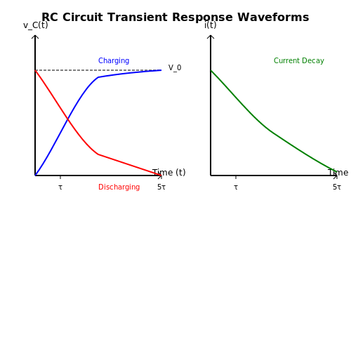
The transient response is often plotted as voltage vs. time, showing the exponential approach to steady state. For AC analysis, Bode plots illustrate the frequency-dependent gain and phase shift.

3.1 RC Circuits in Filter Design

RC circuits are fundamental building blocks in analog filter design, leveraging the frequency-dependent impedance of capacitors to shape signal responses. The simplest first-order RC filter can be configured as either a low-pass or high-pass filter, depending on the placement of the capacitor relative to the resistor.

Transfer Function of a First-Order RC Filter

For a low-pass RC filter, the output is taken across the capacitor. The transfer function H(ω) in the frequency domain is derived from the voltage divider principle:

This can be rewritten in terms of magnitude and phase:

The cutoff frequency f_c, where the output power drops to half (-3 dB), is given by:

High-Pass RC Filter

For a high-pass configuration, the output is taken across the resistor. The transfer function becomes:

Its magnitude and phase responses are:

Practical Considerations in Filter Design

While first-order RC filters are simple, they exhibit a shallow roll-off of -20 dB/decade beyond the cutoff frequency. For steeper attenuation, higher-order filters (e.g., Butterworth, Chebyshev) are constructed by cascading multiple RC stages or using active components like op-amps.

Key design trade-offs include:

• Component tolerance: Variations in R and C values shift the cutoff frequency.
• Source and load impedance: Loading effects can alter the filter response.
• Phase distortion: Nonlinear phase response may affect signal integrity in time-critical applications.

Applications in Signal Processing

RC filters are ubiquitous in:

• Anti-aliasing: Low-pass filters prevent high-frequency noise from distorting sampled signals.
• DC blocking: High-pass filters remove DC offsets in AC-coupled amplifier stages.
• Noise suppression: Bandwidth-limiting filters reduce electromagnetic interference (EMI) in sensitive circuits.

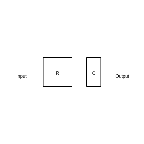
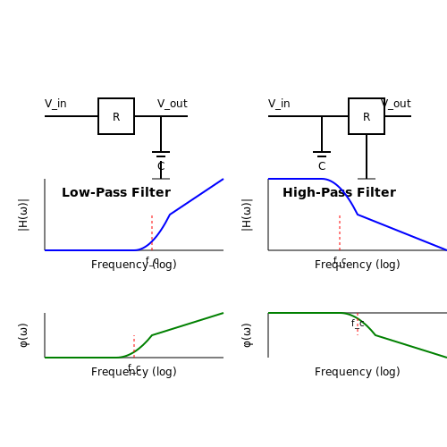
The above diagram illustrates a passive RC low-pass filter. The resistor and capacitor form a voltage divider whose impedance ratio varies with frequency.

3.2 Timing Circuits and Pulse Shaping

Fundamentals of RC Timing Circuits

The time constant (τ) of an RC circuit governs its transient response, defined as:

where R is resistance in ohms and C is capacitance in farads. For a step input, the capacitor voltage V_C(t) follows:

Conversely, during discharge, the voltage decays as:

These equations form the basis for timing applications, where τ determines delays or pulse widths. For instance, in monostable multivibrators, the output pulse duration is directly proportional to τ.

Pulse Shaping with Differentiator and Integrator Circuits

RC networks can shape pulses by exploiting their frequency-dependent behavior:

Differentiator (High-Pass Filter)

When τ ≪ T (input pulse width), the circuit approximates a differentiator. The output voltage across the resistor is:

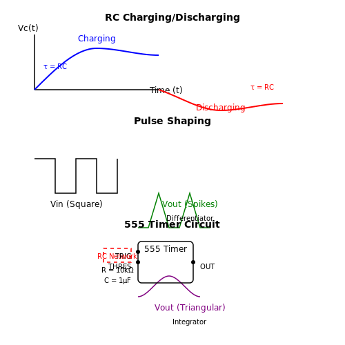
This sharpens edges and converts square waves into narrow spikes, useful in edge detection or clock synchronization.

Integrator (Low-Pass Filter)

When τ ≫ T, the circuit acts as an integrator. The capacitor voltage approximates:

This smoothes rapid transitions, converting square waves into triangular or sawtooth waveforms, often used in analog computing or PWM generation.

Practical Timing Applications

Monostable Multivibrators: A trigger pulse initiates a single output pulse with duration T ≈ 1.1RC. Used in debouncing switches or generating fixed-width pulses.

Astable Multivibrators: Two RC networks create a free-running oscillator. The period depends on charging/discharging times:

Schmitt Triggers: Hysteresis combined with RC feedback produces clean square waves from noisy inputs, critical in signal conditioning.

Non-Ideal Effects and Compensation

Source Impedance: Non-zero output resistance of the driving stage alters effective τ. Compensate by ensuring R_source ≪ R.

Capacitor Leakage: Real capacitors exhibit leakage resistance, modifying discharge characteristics. Use low-leakage types (e.g., ceramic or film) for precision timing.

Propagation Delays: In fast-edge applications, parasitic inductance and capacitance introduce jitter. Minimize loop area and use controlled-impedance layouts.

Case Study: 555 Timer IC

The 555 timer exemplifies RC timing principles. In monostable mode, the output pulse width is:

where R_A is the timing resistor. Astable mode oscillation frequency depends on both resistors and capacitor:

This versatility makes the 555 ubiquitous in pulse generation, LED flashers, and tone generators.

3.3 Integrator and Differentiator Circuits

Basic Operational Principles

An RC integrator produces an output voltage proportional to the integral of the input signal, while a differentiator generates an output proportional to the derivative of the input. These behaviors arise from the time-dependent voltage-current relationship in capacitors, governed by:

For an integrator, the output voltage is taken across the capacitor, leading to:

Conversely, a differentiator measures voltage across the resistor, yielding:

Practical Circuit Implementations

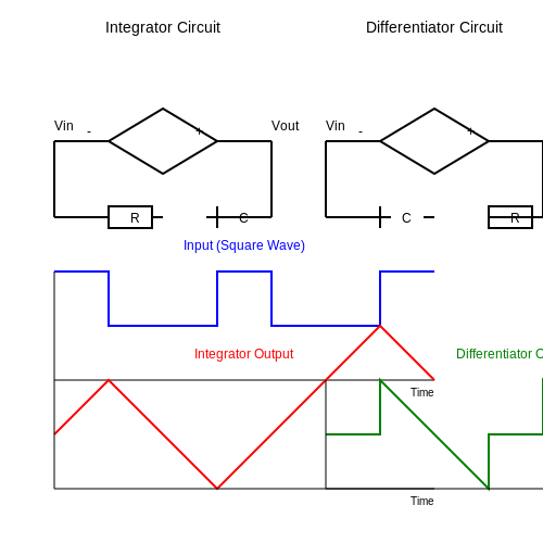
The ideal integrator uses an operational amplifier in an inverting configuration with a capacitor in the feedback path:

The differentiator swaps these components, placing the capacitor at the input. Both circuits require careful consideration of the time constant τ = RC relative to the input signal frequency.

Frequency Response Analysis

The transfer function for an integrator in the frequency domain is:

Exhibiting a -20 dB/decade slope and constant -90° phase shift. The differentiator's transfer function:

Produces a +20 dB/decade gain slope with a constant +90° phase shift. Practical implementations often include a parallel resistor with the feedback capacitor (integrator) or series resistor with the input capacitor (differentiator) to limit high-frequency gain.

Applications and Limitations

Integrators find use in:

• Analog computing (solving differential equations)
• Waveform generation (triangular waves from square waves)
• PID controllers (integral term implementation)

Differentiators are employed in:

• Edge detection in pulse signals
• Frequency modulation circuits
• Rate-of-change measurements

Non-ideal effects include:

• Op-amp bandwidth limitations causing phase errors
• Capacitor leakage currents introducing DC drift
• Stability issues with high-frequency noise amplification

Design Considerations

The cutoff frequency f_c must be carefully selected:

For integrators, f_c should be below the lowest frequency component of interest. Differentiators require f_c above the highest significant frequency to prevent excessive high-frequency noise amplification. Component tolerances critically affect performance - film capacitors and metal-film resistors are preferred for precision applications.

4.1 Differential Equations Governing RC Circuits

The behavior of an RC (resistor-capacitor) circuit is governed by first-order linear differential equations derived from Kirchhoff's laws and the constitutive relations of the circuit elements. These equations describe how voltage and current evolve over time in response to input signals, whether step, sinusoidal, or arbitrary waveforms.

Derivation of the RC Circuit Equation

Consider a simple series RC circuit with a voltage source V(t), resistor R, and capacitor C. Applying Kirchhoff's voltage law (KVL) around the loop gives:

where V_R(t) is the voltage across the resistor and V_C(t) is the voltage across the capacitor. Using Ohm's law and the capacitor's current-voltage relationship, we substitute:

To eliminate the integral, differentiate both sides with respect to time:

This is a first-order linear differential equation in terms of the current i(t). Alternatively, we can express the equation in terms of the capacitor voltage V_C(t) by noting that i(t) = C dV_C(t)/dt:

This standard form highlights the time constant τ = RC, which governs the transient response of the circuit.

Solution to the Differential Equation

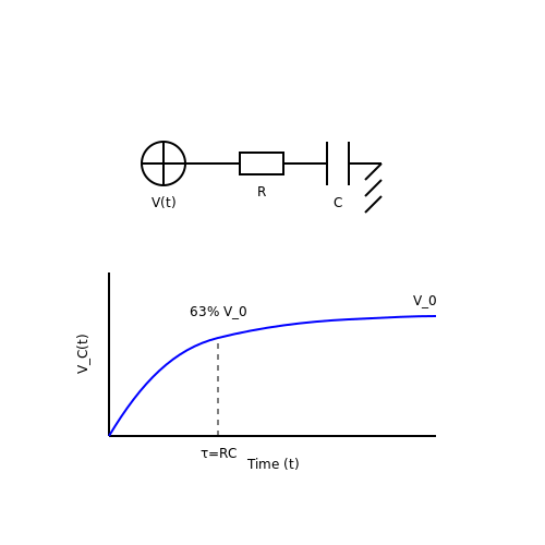
The general solution to the first-order differential equation consists of a homogeneous (transient) solution and a particular (steady-state) solution. For a constant input voltage V(t) = V_0, the homogeneous equation is:

The solution to this equation is an exponential decay:

where A is determined by initial conditions. For a step input at t = 0 with V_C(0) = 0, the complete solution becomes:

This describes the classic exponential charging curve of an RC circuit, reaching approximately 63% of V_0 after one time constant τ = RC.

Time Constant and Practical Implications

The time constant τ = RC is a critical parameter that determines:

• The rise/fall time of pulse responses
• The cutoff frequency in filter applications (f_c = 1/(2πRC))
• The settling time for the circuit to reach steady state

In practical applications, engineers select R and C values to achieve desired timing characteristics. For instance, in timer circuits or noise filtering, specific time constants are chosen to match the required operational bandwidth.

Frequency Domain Analysis

While the time-domain differential equation provides complete information about the circuit's behavior, the frequency domain approach using impedance (Z_R = R, Z_C = 1/jωC) often simplifies analysis for sinusoidal inputs. The transfer function of the RC circuit's output voltage is:

This represents a low-pass filter characteristic with a -3dB cutoff frequency at ω = 1/RC.

The differential equation approach remains fundamental for analyzing circuits with non-sinusoidal or time-varying inputs where frequency domain methods are less straightforward to apply.

4.2 Laplace Transform Analysis

The Laplace transform provides a powerful method for analyzing RC circuits in the frequency domain, simplifying the solution of differential equations into algebraic manipulations. For an RC circuit, the voltage-current relationship in the time domain is governed by:

Applying the Laplace transform converts this integro-differential equation into an algebraic form. The key transforms used are:

• Resistor: V(s) = RI(s)
• Capacitor: V(s) = I(s)/(sC)
• Inductor: V(s) = sLI(s) (for completeness, though not present in pure RC circuits)

Transfer Function Derivation

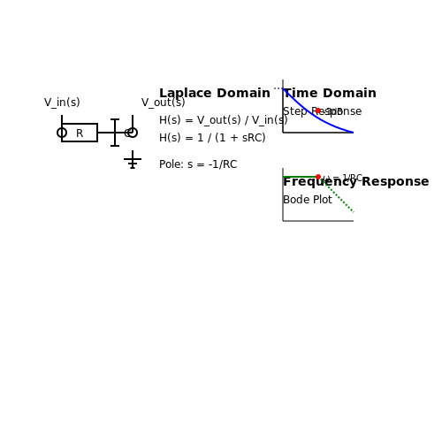
Consider a simple series RC circuit with input voltage V_in(s) and output voltage V_out(s) across the capacitor. The impedance divider gives:

This first-order low-pass filter has a pole at s = -1/RC. The time constant τ = RC appears naturally in the Laplace domain analysis.

Step Response Analysis

For a unit step input V_in(s) = 1/s, the output becomes:

Partial fraction expansion yields:

Taking the inverse Laplace transform gives the familiar exponential charging curve:

Frequency Response

Substituting s = jω in the transfer function reveals the frequency-dependent behavior:

The magnitude and phase responses are:

The -3dB cutoff frequency occurs at ω_c = 1/RC, demonstrating how Laplace analysis seamlessly connects time and frequency domain behavior.

Pole-Zero Interpretation

The single pole at s = -1/RC determines the circuit's transient response. A Bode plot of the system shows:

• 20dB/decade roll-off above the cutoff frequency
• Phase shift from 0° to -90°
• Maximum group delay at the pole frequency

This analysis extends to more complex RC networks by treating them as systems of equations in the s-domain, where series and parallel impedances combine algebraically.

4.3 Frequency Domain Representation

The frequency domain representation of an RC circuit provides critical insights into its behavior under sinusoidal excitation, revealing how amplitude and phase vary with frequency. Unlike time-domain analysis, which examines transient responses, frequency-domain analysis focuses on steady-state behavior using tools like the Fourier transform and Bode plots.

Transfer Function of an RC Circuit

The transfer function H(ω) of a series RC circuit relates the output voltage (across the capacitor) to the input voltage. Starting from the impedance of the capacitor Z_C = 1/(jωC) and resistor Z_R = R, the voltage divider rule yields:

Simplifying this expression:

This is a first-order low-pass filter transfer function, where the cutoff frequency ω_c = 1/(RC) (or f_c = 1/(2πRC)) marks the boundary between the passband and stopband.

Magnitude and Phase Response

The magnitude |H(ω)| and phase φ(ω) of the transfer function are derived by converting H(ω) to polar form:

Key observations:

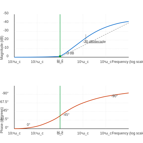
• At low frequencies (ω ≪ ω_c): |H(ω)| ≈ 1 (0 dB) and φ(ω) ≈ 0°, meaning the output closely follows the input.
• At the cutoff frequency (ω = ω_c): |H(ω)| = 1/√2 ≈ 0.707 (−3 dB) and φ(ω) = −45°.
• At high frequencies (ω ≫ ω_c): |H(ω)| ≈ 1/(ωRC) (rolls off at −20 dB/decade) and φ(ω) ≈ −90°.

Bode Plot Analysis

A Bode plot visualizes the magnitude (in decibels) and phase (in degrees) as functions of logarithmic frequency. For an RC low-pass filter:

• Magnitude plot: Flat at 0 dB until ω_c, then decreases linearly at −20 dB/decade.
• Phase plot: Transition from 0° to −90°, with a −45° shift at ω_c.

Applications in Signal Processing

The frequency-domain representation is pivotal in designing filters, impedance matching networks, and noise reduction circuits. For example:

• Anti-aliasing filters: RC circuits precondition signals before analog-to-digital conversion to prevent high-frequency artifacts.
• AC coupling: High-pass RC filters block DC components while transmitting AC signals.

Engineers leverage these principles in audio systems, telecommunications, and control systems, where frequency-selective behavior is critical.

5.1 Recommended Textbooks

• PDF EE 233 Circuit Theory Lab 1: RC Circuits - University of Washington — EE 233 Lab 1: RC Circuits Laboratory Manual Page 2 of 11 3 Prelab Exercises 3.1 The RC Response to a DC Input 3.1.1 Charging RC Circuit The differential equation for out( ) is the most fundamental equation describing the RC circuit, and it can be solved if the input signal in( ) and an initial condition are given. Prelab #1:
• PDF RC Circuits - Michigan State University — 5. RC Circuits VC =V0 1−e−1 ≈0.63V0 (5.4) VR =V0 e−1 ≈0.37V0 (5.5) This means that after t = τ seconds, the capacitor has been charged to63 ...
• PDF Fundamentals of Electronic Circuit Design - University of Cambridge — 1.6 Electronic Circuits as Linear Systems 2 Fundamental Components: Resistors, capacitors, and Inductors 2.1 Resistor 2.2 Capacitors 2.3 Inductors 3 Impedance and s-Domain Circuits 3.1 The Notion of Impedance 3.2 The Impedance of a Capacitor 3.3 Simple RC filters 3.4 The Impedance of an Inductor 3.5 Simple RL Filters 3.6 s-Domain Analysis
• The Best Online Library of Electrical Engineering Textbooks — Electronics textbooks including: Fundamentals of Electrical Engineering, Electromagnetics, Introduction to Electricity, Magnetism, & Circuits and more. ... RC Circuits 6.5; Household Wiring and Electrical Safety 6.6; Chapter 6 ... both this textbook and the Circuits 101 tutorials will provide two different methods of teaching and it is highly ...
• PDF Step Response of RC Circuits - University of Washington — The step response of RC circuits is covered in the textbook. Review the appropriate sections, look at signal waveforms, and review the definition and formula for the time constant. Review the usage of laboratory instruments. 3. Circuits Figure 1 shows a simple circuit of a function generator driving a resistive load. This circuit is used
• PDF Step Response of RC Circuits - UW Faculty Web Server — Figure 2 shows the first-order RC circuit whose step response will be studied in this lab. Figure 3 shows two sections of the first-order RC circuit connected in series to illustrate a simple technique to model computer bus systems (PCI bus, SCSI bus, etc.). Arbitrary waveform Figure 1. Internal resistance of an arbitrary waveform generator.
• Readings | Circuits and Electronics | Electrical Engineering and ... — This section contains the course's reading assignments, which refer to the required textbook: Agarwal, Anant, and Jeffrey H. Lang. Foundations of Analog and Digital Electronic Circuits . San Mateo, CA: Morgan Kaufmann Publishers, Elsevier, July 2005.
• PDF Step Response of RC Circuits - dunham.ece.uw.edu — • Calculate and measure various timing parameters of switching waveforms (time constant, delay time, rise time, and fall time) common in computer systems. • Compare theoretical calculations and experimental data, and explain any discrepancies. 2. Reference The step response of RC circuits is covered in the textbook.
• Chapter 5: Basic Signals and Waveform Synthesis - GlobalSpec — Electrical engineers normally consider a signal to be an electric current or voltage, and these currents and voltages are functions of time. The step, ramp, impulse, exponential, and sinusoidal functions, etc., are the basic signals. These signals may be combined by addition or subtraction to build a variety of general waveforms used in practice.
• PDF LTspice Essentials - content.e-bookshelf.de — degree in electronic engineering, an MSc degree in automatic control engineering, and a PhD degree in digital signal processing. Dogan has worked in many industrial organizations before he returned to academic life. Prof Ibrahim is the author of over 70 technical books and published over 200 technical articles on microcontrollers,

5.2 Online Resources and Tutorials

• NI Circuits (3e) | Interactive Digital Courseware from zyBooks — 5.1 Nonperiodic waveforms 5.2 Capacitors 5.3 Series and parallel capacitors 5.4 Technology brief: Supercapacitors 5.5 Inductors 5.6 Series and parallel Inductors 5.7 RC natural response 5.8 RC forced response 5.9 RC Thévenin equivalents 5.10 Measuring the time constant 5.11 Response of the RL circuit 5.12 Technology brief: Hard disk drives (HDD)
• PDF ECE 2120 Electrical Engineering Laboratory II - Clemson University — Lab 3 - Capacitors and Series RC Circuits 9 Lab 4 - Inductors and Series RL Circuits 18 Lab 5 - Parallel RC and RL Circuits 25 Lab 6 - Circuit Resonance 33 Lab 7 -Filters: High-pass, Low-pass, Bandpass, and Notch 42 Lab 8 - Transformers 52 Lab 9 - Two-Port Network Characterization 61 Lab 10 - Final Exam 70 Appendix A - Safety 72
• PDF EE 233 Circuit Theory Lab 1: RC Circuits - University of Washington — EE 233 Lab 1: RC Circuits Laboratory Manual Page 2 of 11 3 Prelab Exercises 3.1 The RC Response to a DC Input 3.1.1 Charging RC Circuit The differential equation for out( ) is the most fundamental equation describing the RC circuit, and it can be solved if the input signal in( ) and an initial condition are given. Prelab #1:
• 5.2: Activities - Physics LibreTexts — - Open the laptop computer file "RC_Circuits," and click the ON button in the Signal Generator window. Place the scope leads across the Output 1 signal generator outputs of the Pasco box, black to , and red to . Play around with the onscreen Waveform, Frequency and Amplitude settings (in the interest of efficiency, 2 or 3 waveforms should ...
• PDF RC Circuits - Michigan State University — 5. RC Circuits VC =V0 1−e−1 ≈0.63V0 (5.4) VR =V0 e−1 ≈0.37V0 (5.5) This means that after t = τ seconds, the capacitor has been charged to63 ...
• PDF Step Response of RC Circuits - University of Washington — - 4 - amplitude on the front panel reflects this assumption. The output voltage Vout might be very different to V s depending on the resistive load R 1. 5.2 Step response and timing parameters The step response of a simple RC circuit, illustrated in Figure 4, is an exponential signal with time
• PDF Step Response of RC Circuits - dunham.ece.uw.edu — The step response of a simple RC circuit, illustrated in Figure 4, is an exponential signal with time constant τ = RC. Besides this timing parameter, four other timing parameters are important in describing how fast or how slow an RC circuit responds to a step input. These timing parameters are marked in Figure 4, at three voltage levels: a.
• PDF Step Response of RC Circuits - UW Faculty Web Server — Figure 2 shows the first-order RC circuit whose step response will be studied in this lab. Figure 3 shows two sections of the first-order RC circuit connected in series to illustrate a simple technique to model computer bus systems (PCI bus, SCSI bus, etc.). Arbitrary waveform Figure 1. Internal resistance of an arbitrary waveform generator.
• PDF Laboratory - 5 Waveforms and Signals — produce a sawtooth waveform. The circuit for doing this is shown in Figure 5.10. Figure 5.10 Circuit for producing a sawtooth waveform. The period of the sawtooth wave can be adjusted using either E, C or R. The amplitude is fixed at the value of the relay pick-up voltage, V operate. One can obtain a larger amplitude for the sawtooth
• LAB 6: RC CIRCUITS; PASSIVE FILTERS - New Jersey Institute of Technology — Check if the time constants on the rising and the falling parts of the waveform are the same. Make sure that you apply a square wave of low enough frequency so that the output waveform becomes flat before the input waveform changes polarity. HINT: To measure the time constant t, use the cursors on the digital scope screen. The scope may also ...

5.3 Research Papers and Advanced Readings

• PDF BEE 233 Circuits Fall 2015 Lab 2: RC circuits - University of Washington — Lab 2: RC circuits 1 Objectives 1. Measure the output waveform of simple RC circuits excited by step functions. 2. Calculate and measure various timing parameters, including the time constant, rise and fall times and the propagation delays. 3. Compare expected and experimentally measured values. 2 First and second order RC circuits
• PDF ECE 2120 Electrical Engineering Laboratory II - Clemson University — Lab 3 - Capacitors and Series RC Circuits 9 Lab 4 - Inductors and Series RL Circuits 18 Lab 5 - Parallel RC and RL Circuits 25 Lab 6 - Circuit Resonance 33 Lab 7 -Filters: High-pass, Low-pass, Bandpass, and Notch 42 Lab 8 - Transformers 52 Lab 9 - Two-Port Network Characterization 61 Lab 10 - Final Exam 70 Appendix A - Safety 72
• Millman Pulse and Digital Circuits - Academia.edu — The RC Coupled Amplifier Stage 3-2. Steady-state Analysis of an Amplifier 3-3. Amplitude and Time-delay Response of an RC Coupled Amplifier S~ge 3-4. Unit Step Response of an Amplifier. 3-5. Transient Response of an RC Coupled Amplifier Stage 3-6.
• Sinusoidal Oscillators and Waveform Generators Using Modern Electronic ... — Sinusoidal Oscillators and Waveform Generators Using Modern Electronic Circuit Building Blocks ( PDFDrive ) - Free ebook download as PDF File (.pdf), Text File (.txt) or read book online for free. ... popular topic of research in the Circuits and Systems literature. Consequently, well over 1500 research papers have so far been published on ...
• CIS 6930.3753X Spr.'02: Part V Readings - cise.ufl.edu — The following papers describe a resonant clock-waveform generation technique. Although these papers focus on square wave generation, the same technique can also be used to approximate any desired periodic waveform, including the trapezoidal waveforms required for driving adiabatic circuits. ... Additional readings: The paper that introduces the ...
• PDF ELECTRICAL CIRCUIT ANALYSIS Lecture Notes - MRCET — (t)/dt + (1/RC). v C (t) = V/RC The inverse coefficient of v C (t) is known as the time constant of the circuit τand is given by τ = RC and it's units are seconds. The above equation is a first order differential equation and can be solved by using the same method of separation of variablesas we adopted for the LC circuit.
• PDF Step Response of RC Circuits - University of Washington — The step response of a simple RC circuit, illustrated in Figure 4, is an exponential signal with time constant τ = RC. Besides this timing parameter, four other timing parameters are important in describing how fast or how slow an RC circuit responds to a step input. These timing parameters are marked in Figure 4, at three voltage levels: a.
• Siam J. 2, - Jstor — TRANSMISSION CONDITIONS IN WR FOR RC CIRCUITS 1077 X\ R\ X2 Rn—Ί %n—l R-n—l η-vWV X\ R\ X2 Rn—2 Xn—\ Rn—1 Xfl VWV—r— \A/W-WW Rn-1> -TVn-!Rn> jCn 4=0 %.Ri Fig. 1. Ourmodel RC circuit. paper, we present atheoretical foundation for the determinationofthe optimization parameter for the important classofdiffusive RC circuits. Circuit equations are often specified in terms of the ...
• PDF Step Response of RC Circuits - dunham.ece.uw.edu — The step response of a simple RC circuit, illustrated in Figure 4, is an exponential signal with time constant τ = RC. Besides this timing parameter, four other timing parameters are important in describing how fast or how slow an RC circuit responds to a step input. These timing parameters are marked in Figure 4, at three voltage levels: a.
• Sinusoidal Oscillators and Waveform Generators using Modern Electronic ... — Printed on acid-free paper Springer International Publishing AG Switzerland is part of Springer ScienceþBusiness Media (www.springer.com) Preface Sinusoidal oscillators and waveform generators have numerous applications in electronics, instrumentation, measurement, communications, control systems, and signal processing, due to which they have ...