Negative Feedback Systems
1. Definition and Basic Concept of Negative Feedback
1.1 Definition and Basic Concept of Negative Feedback
Negative feedback is a control mechanism where a portion of the output signal is fed back into the system's input with an inverted phase, reducing deviations from the desired operating point. This principle stabilizes the system by counteracting perturbations, improving linearity, bandwidth, and distortion characteristics.
Mathematical Formulation
Consider an open-loop amplifier with gain A. When negative feedback is applied, the feedback factor β determines the fraction of output returned to the input. The closed-loop gain Af becomes:
For large loop gain (Aβ ≫ 1), the system approximates:
This demonstrates how negative feedback makes the system behavior dependent primarily on the passive feedback network rather than the active components.
Key Properties
- Stability Enhancement: Reduces sensitivity to parameter variations in active components
- Bandwidth Extension: The gain-bandwidth product remains constant, so reduced gain increases bandwidth
- Noise Reduction: Suppresses noise originating within the forward path
- Linearity Improvement: Decreases harmonic distortion through error correction
Practical Implementation
In operational amplifier circuits, negative feedback manifests through configurations like:
- Inverting amplifier: Feedback through impedance network
- Non-inverting amplifier: Voltage divider feedback
- Transimpedance amplifier: Current-to-voltage conversion
The phase relationship proves critical - true negative feedback requires 180° phase shift around the loop at the operating frequency. Systems violating this condition may oscillate, transforming into positive feedback configurations.
Historical Context
Harold S. Black's 1927 patent established the modern concept while developing stable telephone amplifiers. The discovery enabled long-distance communication by solving distortion problems in vacuum tube amplifiers. Later refined by Bode's work on stability criteria, negative feedback became fundamental across control systems and analog electronics.

Key Components of a Negative Feedback System
Error Detector (Comparator)
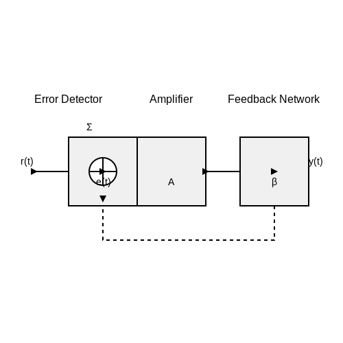
A negative feedback system fundamentally relies on an error detector, which compares the system's output with the reference input. The difference between these signals, known as the error signal, drives the system toward equilibrium. In operational amplifier (op-amp) circuits, this is often implemented using a differential amplifier. The error signal e(t) is given by:
where r(t) is the reference input and y(t) is the feedback signal. High-precision comparators, such as those in instrumentation amplifiers, minimize offset errors to ensure accurate feedback control.
Amplifier (Forward Path Gain)
The forward path amplifier processes the error signal to produce the system output. Its gain A determines the open-loop response. In electronic systems, this is typically an op-amp or transistor-based amplifier. The output y(t) is:
Nonlinearities in the amplifier, such as saturation or crossover distortion, can degrade performance, necessitating careful design to maintain linear operation within the desired range.
Feedback Network
The feedback network samples the output and feeds a portion back to the input. This network, often a resistive divider in analog circuits, defines the feedback factor β. For a voltage divider:
In control systems, β may include dynamic elements (e.g., capacitors or inductors) for frequency-dependent behavior. Stability analysis requires evaluating the loop gain Aβ across all frequencies.
Summing Junction (Mixing Point)
The summing junction combines the reference input and feedback signal. In analog circuits, this is often a virtual ground node in op-amp configurations. Kirchhoff's current law governs the mixing process:
Digital implementations use arithmetic logic units (ALUs) for discrete-time signal processing. Phase matching at this junction is critical to avoid instability in high-frequency systems.
Compensation Networks
To mitigate instability, compensation networks shape the system's frequency response. Techniques include:
- Dominant pole compensation: Introduces a low-frequency pole to roll off gain before phase shift reaches 180°.
- Lead-lag compensation: Combines lead (phase boost) and lag (gain reduction) networks for optimized transient response.
The compensated loop gain T(s) must satisfy the Nyquist stability criterion:
Practical Considerations
Real-world implementations must account for:
- Non-ideal components: Finite input impedance, output resistance, and parasitic capacitances alter expected behavior.
- Noise susceptibility: Feedback can amplify high-frequency noise if not properly filtered.
- Thermal drift: Resistor temperature coefficients affect β in precision applications.
For example, in a precision voltage regulator, 0.1% tolerance resistors and low-drift op-amps maintain β stability over temperature variations.
1.3 Mathematical Representation of Feedback Loops
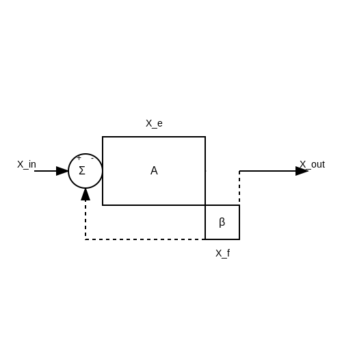
The mathematical modeling of negative feedback systems provides a rigorous framework for analyzing stability, gain, and distortion. The fundamental structure consists of an open-loop amplifier with gain A and a feedback network with transfer function β.
Closed-Loop Gain Derivation
Consider a basic feedback system where the input signal Xin is compared with the feedback signal Xf to produce an error signal Xe:
The forward path amplifies this error:
While the feedback path scales the output:
Substituting these relationships yields the classic closed-loop gain equation:
Loop Gain and Stability Criteria
The term Aβ, called the loop gain, determines system behavior:
- For |1 + Aβ| > 1, the system exhibits negative feedback
- When Aβ = -1, the denominator becomes zero causing oscillation (Barkhausen criterion)
- The phase margin is determined by the frequency where |Aβ| = 1
Frequency Domain Analysis
For practical systems, we express the transfer function in the Laplace domain:
Where A(s) typically includes poles from amplifier bandwidth limitations:
Sensitivity and Distortion Reduction
Negative feedback reduces sensitivity to parameter variations in the forward path. The sensitivity function S quantifies this:
Harmonic distortion components are similarly attenuated by the loop gain factor.
Practical Design Considerations
In operational amplifier circuits, the feedback network often consists of resistors establishing:
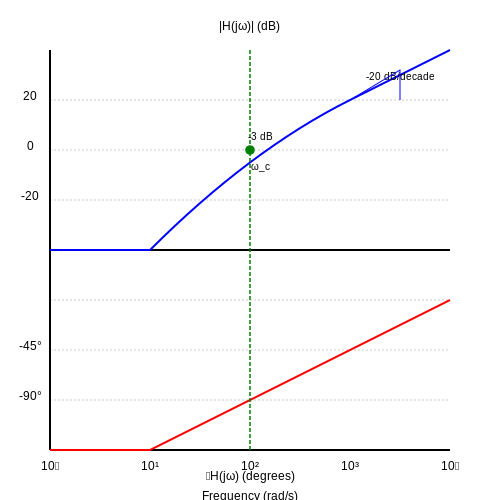
Stability analysis requires examining the Bode plot of A(jω)β(jω), ensuring adequate phase margin (typically >45°) at the unity-gain frequency.
2. Stabilization of System Performance
2.1 Stabilization of System Performance
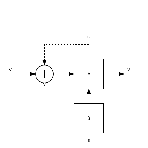
Negative feedback inherently stabilizes system performance by reducing sensitivity to parameter variations, noise, and nonlinearities. Consider a forward-path gain A and feedback factor β. The closed-loop gain G is given by:
For large loop gain (Aβ ≫ 1), the system becomes primarily dependent on β, which is typically a stable, passive component. This reduces the impact of forward-path uncertainties. To quantify stabilization, analyze the sensitivity function S, defined as the fractional change in closed-loop gain relative to fractional changes in A:
Reduction of Nonlinear Distortion
Nonlinearities in amplifiers (e.g., transistor saturation) introduce harmonic distortion. Negative feedback linearizes the response by attenuating distortion components. If the open-loop system produces distortion D, the closed-loop distortion DCL becomes:
Bandwidth Extension
Feedback trades gain for bandwidth. A single-pole amplifier with open-loop bandwidth f0 and DC gain A0 exhibits a closed-loop bandwidth fCL:
This arises because the gain-bandwidth product remains constant: A0f0 = GfCL.
Noise Suppression
Feedback minimizes the impact of additive noise in the forward path. For noise N injected at the amplifier input, the output noise Nout is:
Practical implementations, such as operational amplifiers, leverage these principles to achieve stable gain across temperature variations and manufacturing tolerances.
Case Study: Op-Amp Frequency Compensation
Dominant-pole compensation ensures stability by enforcing a 20 dB/decade rolloff before the phase margin drops critically. The compensated open-loop transfer function A(s) is:
where ωp is the dominant pole and ω2 is a secondary pole. Feedback forces the closed-loop response to track 1/β until the loop gain crosses 0 dB.
2.2 Reduction of Nonlinear Distortion
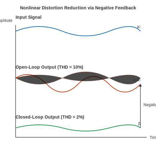
Nonlinear distortion arises when an amplifier's transfer characteristic deviates from ideal linearity, generating harmonic and intermodulation products. In open-loop configurations, this manifests as gain variations with input amplitude, producing unwanted spectral components. Negative feedback dramatically reduces such distortion by enforcing a linear relationship between input and output.
Mathematical Analysis of Distortion Reduction
Consider an amplifier with an open-loop nonlinear transfer characteristic:
where a1 represents the linear gain and a2, a3 characterize second and third-order nonlinearities. When negative feedback with factor β is applied, the closed-loop output becomes:
The key observation is that nonlinear terms are suppressed by higher powers of the feedback factor (1 + a1β). For substantial loop gain (a1β ≫ 1), harmonic distortion components decrease as:
Practical Implications
In audio power amplifiers, negative feedback reduces total harmonic distortion (THD) from several percent to 0.01% or lower. The technique proves particularly effective against:
- Crossover distortion in Class B output stages
- Transconductance nonlinearity in differential pairs
- Early effect in bipolar transistors
However, the distortion reduction is ultimately limited by the loop gain's frequency response. As phase margin decreases at higher frequencies, the feedback becomes less effective at suppressing distortion in wideband signals.
Intermodulation Distortion Considerations
For multi-tone signals, negative feedback similarly reduces intermodulation products. Two-tone analysis shows third-order intercept point (IP3) improvement by:
This relationship explains why feedback amplifiers maintain better linearity in RF systems where spectral regrowth must be minimized.
Limitations and Tradeoffs
While negative feedback effectively reduces memoryless nonlinearities, it cannot compensate for:
- Time-varying distortions (e.g., power supply modulation)
- Nonlinear capacitances in high-frequency designs
- Thermal effects with long time constants
Excessive feedback can also induce conditional stability, where the system becomes susceptible to oscillation near the unity-gain frequency. Careful compensation is required to balance distortion reduction with stability margins.
2.3 Improvement in Bandwidth and Frequency Response
Negative feedback significantly enhances the bandwidth and frequency response of amplifiers by reducing the gain-bandwidth trade-off inherent in open-loop systems. The mechanism stems from the relationship between loop gain and the system's dominant pole frequency. Consider an amplifier with an open-loop transfer function:
where A0 is the DC gain and ωp is the dominant pole frequency. When negative feedback with factor β is applied, the closed-loop gain becomes:
This shows two critical effects:
- The DC gain reduces by the feedback factor (1 + βA0)
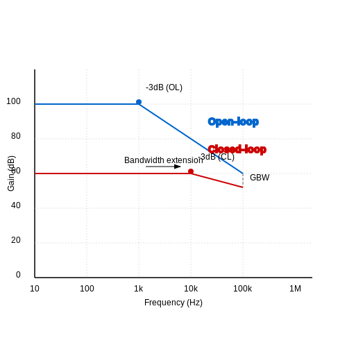
- The bandwidth increases by the same factor, pushing the -3dB point to ωp(1 + βA0)
Gain-Bandwidth Product Conservation
The gain-bandwidth product (GBW) remains constant in a single-pole system:
where Af0 is the closed-loop gain and ωf is the closed-loop bandwidth. This principle enables designers to trade excess gain for extended frequency response - a key advantage in wideband amplifiers and precision measurement systems.
Multi-Pole Systems and Stability
For systems with multiple poles, negative feedback alters the frequency response more complexly. The loop gain βA(s) modifies the pole locations, potentially causing peaking or instability if phase margin is insufficient. The stability criterion requires:
Compensation techniques (e.g., dominant pole placement, Miller compensation) are often employed with feedback to ensure stable operation across the extended bandwidth.
Practical Implications
In operational amplifiers, negative feedback enables:
- Wideband instrumentation amplifiers with flat response up to MHz ranges
- High-speed data converters requiring uniform gain across signal bandwidths
- RF amplification stages where consistent gain over broad frequency ranges is critical
The figure below shows a typical frequency response comparison between open-loop and closed-loop configurations:
3. Voltage-Series Feedback
3.1 Voltage-Series Feedback
Voltage-series feedback, also known as series-shunt feedback, is a configuration where the feedback network samples the output voltage and returns a proportional voltage in series with the input. This topology is widely used in amplifiers to stabilize gain, reduce distortion, and improve input/output impedance characteristics.
Basic Configuration
The feedback network consists of a voltage divider (R1 and R2) connected between the output and the input. The feedback factor (β) is given by:
where Vf is the feedback voltage and Vo is the output voltage. The closed-loop gain (Af) of the amplifier with feedback is derived from the open-loop gain (Av) as:
For large loop gain (βAv ≫ 1), the closed-loop gain simplifies to 1/β, making the system highly stable against variations in transistor parameters or supply voltage.
Input and Output Impedance Effects
Voltage-series feedback increases the input impedance and decreases the output impedance, making the amplifier more suitable for voltage amplification. The modified impedances are:
where Zin and Zout are the open-loop input and output impedances, respectively.
Practical Applications
This configuration is commonly found in:
- Operational amplifiers (non-inverting mode)
- Audio power amplifiers (for distortion reduction)
- Voltage regulators (to maintain stable output)
Stability Considerations
While voltage-series feedback improves linearity, it can introduce phase shifts at high frequencies, risking instability. Compensation techniques, such as dominant-pole compensation or Miller compensation, are often employed to ensure stability across the operating bandwidth.
where φm is the phase margin, critical for avoiding oscillations.

3.2 Voltage-Shunt Feedback
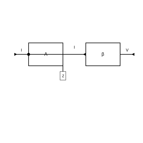
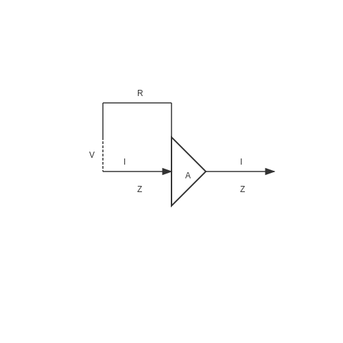
Voltage-shunt feedback, also known as shunt-shunt feedback, is a configuration where the feedback network samples the output voltage and returns a current proportional to it, summing it in shunt at the input. This topology is widely used in transimpedance amplifiers and high-frequency circuits due to its stability and bandwidth enhancement properties.
Basic Configuration
The system consists of an amplifier with open-loop gain A and a feedback network with transimpedance β (units in ohms). The feedback current If is given by:
where Vout is the output voltage. The input current Iin is the sum of the signal current and the feedback current:
Closed-Loop Gain Derivation
The open-loop transimpedance gain Zm relates output voltage to input current:
Substituting the feedback current:
Rearranging terms, the closed-loop transimpedance gain Zm,cl becomes:
For large loop gain (Zmβ ≫ 1), this simplifies to:
Stability and Bandwidth
Voltage-shunt feedback reduces the input and output impedances, improving bandwidth but requiring careful stability analysis. The input impedance Zin,cl and output impedance Zout,cl are given by:
where Zin and Zout are the open-loop impedances. The reduction in impedance enhances high-frequency response but may introduce phase margin concerns.
Practical Applications
- Transimpedance Amplifiers: Used in photodiode circuits to convert current to voltage with low noise.
- High-Frequency Amplifiers: Enhances bandwidth in RF and microwave circuits by reducing impedance.
- Current Feedback Amplifiers (CFAs): Leverages shunt feedback for wideband operation.
Design Considerations
Key trade-offs include:
- Noise Performance: Feedback resistors contribute thermal noise.
- Phase Margin: Requires compensation if loop gain approaches instability.
- Linearity: Feedback improves distortion but depends on β accuracy.
3.3 Current-Series Feedback
Current-series feedback, also known as series-shunt feedback, is a configuration where the feedback network senses the output current and returns a voltage signal in series with the input. This topology is widely used in transconductance amplifiers and current-mode circuits where precise current control is essential.
Basic Operation
The feedback network samples the output current (Io) through a small series resistor (Rf), converting it into a feedback voltage (Vf) proportional to Io. This voltage is then subtracted from the input voltage (Vin), forming a closed-loop system that stabilizes the output current.
The open-loop gain (AOL) of the amplifier is a transconductance (gm), while the feedback factor (β) is determined by the sensing resistor:
Closed-Loop Gain Derivation
The closed-loop transconductance gain (GCL) is derived from the feedback equation:
For large loop gain (gmRf ≫ 1), the closed-loop gain simplifies to:
This result highlights the key advantage of current-series feedback: the transconductance becomes nearly independent of the amplifier's intrinsic parameters, relying instead on the precision of Rf.
Impedance Effects
Current-series feedback increases both the input and output impedances of the amplifier. The modified impedances are given by:
where Zin,OL and Zout,OL are the open-loop input and output impedances, respectively.
Practical Applications
This configuration is commonly found in:
- Current sources: Stabilizes output current against load variations.
- Transconductance amplifiers: Provides precise voltage-to-current conversion.
- RF amplifiers: Enhances linearity and bandwidth.
A classic implementation is the common-emitter amplifier with an emitter degeneration resistor, where Rf corresponds to the emitter resistor (RE).
Stability Considerations
The phase margin of a current-series feedback system depends on the pole locations introduced by the amplifier and feedback network. A dominant pole compensation technique is often employed to ensure stability:
where Ccomp is the compensation capacitor.
3.4 Current-Shunt Feedback
Current-shunt feedback, also known as shunt-series feedback, is a configuration where the feedback network samples the output current and returns a voltage signal in shunt with the input. This topology is widely used in amplifiers to stabilize gain, reduce distortion, and improve bandwidth by controlling the current flow through the feedback loop.
Basic Configuration
The feedback network consists of a shunt resistor (Rf) connected between the output and input nodes. The output current (Iout) develops a voltage across Rf, which is fed back in parallel with the input voltage. The key characteristic is that the feedback signal is proportional to the output current, making it effective for current-mode amplification.
Derivation of Closed-Loop Gain
Let the open-loop current gain of the amplifier be Ai, and the feedback factor β be the ratio of feedback voltage to output current. The closed-loop current gain (Aif) is derived as follows:
Rearranging terms:
Thus, the closed-loop gain becomes:
For large loop gain (Aiβ ≫ 1), the expression simplifies to:
Impedance Effects
Current-shunt feedback reduces the input impedance and increases the output impedance. The modified impedances are calculated as:
This makes the amplifier behave more like an ideal current source at the output while presenting a low impedance at the input.
Practical Applications
Current-shunt feedback is commonly used in:
- Transimpedance amplifiers (e.g., photodiode preamps), where a current input is converted to a voltage output.
- Current-feedback operational amplifiers (CFB Op-Amps), which leverage this topology for wide bandwidth and high slew rate.
- Stabilizing current mirrors in integrated circuits to minimize variations due to process and temperature.
Stability Considerations
Like all feedback systems, current-shunt feedback can introduce instability if the loop gain phase margin is insufficient. Compensation techniques such as dominant-pole placement or Miller compensation are often employed to ensure stability across the operating frequency range.
where fc is the crossover frequency where |Aiβ| = 1.
4. Closed-Loop Gain Calculation
4.1 Closed-Loop Gain Calculation
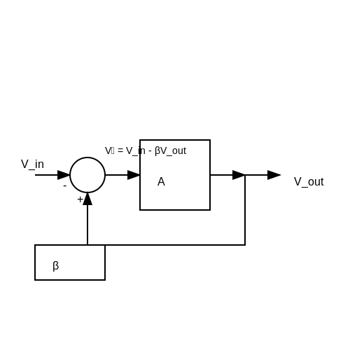
The closed-loop gain ACL of a negative feedback system is a fundamental parameter that determines the amplifier's overall behavior. Unlike open-loop gain, which is highly sensitive to component variations, closed-loop gain remains stable due to feedback.
Derivation of Closed-Loop Gain
Consider a basic feedback system with forward gain A and feedback factor β. The input signal Vin is compared with the feedback signal βVout, producing an error signal Ve = Vin - βVout. The output is then:
Rearranging terms to solve for Vout/Vin yields the closed-loop gain:
Key Observations
- When Aβ ≫ 1, the closed-loop gain simplifies to ACL ≈ 1/β, making the system dependent only on the feedback network.
- The term 1 + Aβ is called the desensitivity factor, quantifying how much variations in A are suppressed.
- Negative feedback trades gain for stability, bandwidth, and linearity.
Practical Example: Non-Inverting Op-Amp
For a non-inverting op-amp with resistors R1 and R2, the feedback factor is β = R1/(R1 + R2). Assuming high open-loop gain (A → ∞), the closed-loop gain becomes:
This result is widely used in precision amplifier designs where predictable gain is critical.
Effect of Finite Open-Loop Gain
For cases where A is not infinitely large, the exact closed-loop gain must account for the finite open-loop gain. For example, if A = 105 and β = 0.01, the closed-loop gain is:
This demonstrates how even with large A, the closed-loop gain slightly deviates from the ideal 1/β = 100.
4.2 Input and Output Impedance Effects
Negative feedback significantly alters the input and output impedance of an amplifier, a critical consideration in circuit design. The feedback topology (series or shunt) determines whether impedances increase or decrease, directly influencing signal transfer efficiency and stability.
Input Impedance Modifications
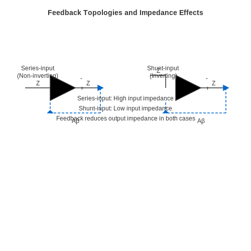
In series-input feedback topologies (e.g., non-inverting op-amp configuration), negative feedback increases the input impedance. The feedback voltage opposes the input signal, reducing the effective voltage across the amplifier's intrinsic input impedance. For an amplifier with open-loop input impedance Zin and loop gain Aβ, the closed-loop input impedance becomes:
Conversely, shunt-input feedback (e.g., inverting op-amp configuration) decreases input impedance. Here, feedback current opposes the input current, effectively lowering the impedance seen by the source:
Output Impedance Modifications
Negative feedback universally reduces output impedance, enhancing an amplifier's ability to drive loads. For an amplifier with open-loop output impedance Zout, the closed-loop output impedance is given by:
This reduction occurs because feedback corrects output voltage variations under load, making the amplifier appear closer to an ideal voltage source. The effect is particularly pronounced in voltage-output topologies.
Practical Implications
Impedance modifications have direct consequences:
- Impedance matching: Series feedback helps interface high-impedance sources to low-impedance loads without signal attenuation.
- Stability: Reduced output impedance minimizes phase shifts caused by capacitive loads, improving stability margins.
- Frequency response: The impedance changes are frequency-dependent due to Aβ's roll-off, affecting bandwidth.
In RF applications, these effects must be carefully modeled using S-parameters, as impedance mismatches can cause reflections and power losses. Modern network analyzers directly measure these closed-loop impedance changes.
Case Study: Op-amp Buffer
A unity-gain buffer (β=1) demonstrates extreme impedance transformation. A typical op-amp with Zin=2 MΩ and Zout=75 Ω at DC, when configured as a buffer with A=105, exhibits:
These values explain why op-amp buffers effectively isolate stages while maintaining signal fidelity. The ultra-low output impedance enables driving transmission lines or multiple parallel loads without signal degradation.
4.3 Stability Analysis and Phase Margin
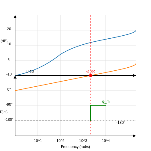
The stability of a negative feedback system is determined by its loop gain characteristics, particularly the phase margin, which quantifies the system's robustness against oscillations. A system is stable if the loop gain magnitude falls below unity before the phase shift reaches -180°.
Nyquist Criterion and Bode Analysis
The Nyquist stability criterion provides a rigorous method for assessing stability by examining the encirclements of the -1 point in the complex plane. However, for practical design, Bode plots offer a more intuitive approach. The phase margin (φm) is defined as:
where T(jωgc) is the loop gain at the gain crossover frequency ωgc (where |T(jωgc)| = 1). A phase margin greater than 45° is typically required for stable operation, with 60° being a common design target for good transient response.
Derivation of Phase Margin Conditions
Consider a second-order system with loop gain:
The phase shift at frequency ω is:
At the gain crossover frequency ωgc, the magnitude condition gives:
Solving for ωgc and substituting into the phase equation yields the phase margin. For dominant pole compensation (ω2 ≫ ω1), this simplifies to:
Practical Implications and Design Trade-offs
In operational amplifier circuits, phase margin directly impacts:
- Overshoot: Lower phase margins increase peaking in the step response.
- Settling time: Margins below 45° cause prolonged ringing.
- Noise rejection: Higher stability improves PSRR and CMRR at high frequencies.
Compensation techniques like pole splitting or Miller compensation are employed to shape the loop gain's frequency response. For example, adding a compensation capacitor Cc introduces a dominant pole at:
while pushing the non-dominant pole to higher frequencies.
Measurement and Simulation Methods
Modern tools enable stability analysis through:
- SPICE AC analysis: Directly plots loop gain magnitude and phase.
- Network analyzers: Inject perturbation signals to measure open-loop response.
- Vector network analyzers (VNAs): Provide precise phase margin measurements up to GHz frequencies.
The following diagram conceptually shows the relationship between phase margin and stability in a Bode plot:
5. Operational Amplifiers and Negative Feedback
Operational Amplifiers and Negative Feedback
Basic Configuration of an Op-Amp with Negative Feedback
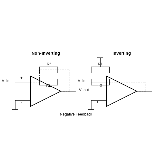
An operational amplifier (op-amp) in a negative feedback configuration stabilizes its output by feeding a portion of the output signal back to the inverting input. The most common configurations include the non-inverting amplifier and the inverting amplifier. For an ideal op-amp with infinite open-loop gain (AOL), the closed-loop gain (ACL) is determined solely by the feedback network.
Derivation of Closed-Loop Gain
For a non-inverting amplifier, the output voltage (Vout) is fed back to the inverting input through a voltage divider formed by R1 and Rf. Applying Kirchhoff's voltage law and the virtual short condition (where V+ ≈ V- due to high open-loop gain), we derive:
Since V- ≈ V+ = Vin, rearranging yields the non-inverting amplifier gain formula.
Impact of Negative Feedback on Performance
Negative feedback improves several key op-amp characteristics:
- Bandwidth Extension: The gain-bandwidth product (GBW) remains constant, but feedback reduces the closed-loop gain, thereby increasing bandwidth.
- Reduced Distortion: Nonlinearities in the op-amp's open-loop response are suppressed.
- Lower Output Impedance: The effective output impedance decreases by a factor of (1 + A_{OL}β), where β is the feedback factor.
- Increased Input Impedance: In non-inverting configurations, input impedance rises significantly due to the virtual short condition.
Stability and Phase Margin
Negative feedback systems must be designed to avoid instability, which occurs when the loop gain (A_{OL}β) introduces a phase shift of 180° at a frequency where the magnitude is unity. The phase margin quantifies stability:
where φ(ωunity) is the phase shift at the frequency where |A_{OL}β| = 1. A phase margin > 45° is typically required for stable operation.
Practical Considerations
Real-world op-amps exhibit limitations such as:
- Slew Rate: The maximum rate of output voltage change, limiting high-frequency performance.
- Input Offset Voltage: A small DC voltage that must be nulled in precision circuits.
- Common-Mode Rejection Ratio (CMRR): The ability to reject signals common to both inputs.
Applications of Negative Feedback in Op-Amps
Negative feedback is ubiquitous in analog circuits, including:
- Active Filters: Sallen-Key and Butterworth configurations rely on feedback for precise frequency response.
- Instrumentation Amplifiers: High-precision differential amplifiers use feedback to reject common-mode noise.
- Oscillators: Wien bridge and phase-shift oscillators employ controlled feedback to sustain oscillations.
5.2 Audio Amplifiers and Signal Processing
Negative feedback plays a critical role in audio amplifier design, where linearity, bandwidth, and distortion reduction are paramount. By feeding a portion of the output signal back into the input with inverted phase, the system can correct for nonlinearities introduced by active components such as transistors or vacuum tubes.
Feedback in Audio Amplifier Topologies
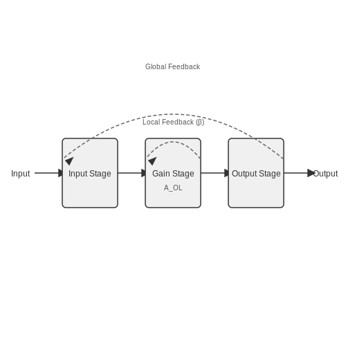
In a typical class-AB audio amplifier, negative feedback is applied globally from the output stage to the differential input pair. The closed-loop gain ACL is determined by the feedback factor β and open-loop gain AOL:
For large AOL, this simplifies to ACL ≈ 1/β, making the system gain primarily dependent on passive components (resistors, capacitors) rather than active device characteristics. This significantly reduces harmonic distortion and output impedance.
Distortion Analysis
Total harmonic distortion (THD) is improved by the feedback factor. If the open-loop distortion is DOL, the closed-loop distortion becomes:
In practical designs, this allows high-end audio amplifiers to achieve THD figures below 0.001% across the audio band (20 Hz - 20 kHz). The feedback network must be carefully compensated to maintain stability, typically using dominant-pole compensation.
Noise Performance
While negative feedback reduces distortion, its effect on noise depends on where the noise enters the system. Input-referred noise is unaffected by feedback, while output-stage noise is attenuated by the feedback factor. The signal-to-noise ratio (SNR) improvement can be expressed as:
This makes feedback particularly valuable in low-noise preamplifier stages where microphone or phono cartridge signals may be in the microvolt range.
Practical Implementation Considerations
Real-world audio amplifiers must balance several competing factors:
- Phase margin: Typically designed for 45-60° to avoid ringing or oscillation
- Slew rate: Feedback cannot correct for slew-induced distortion, requiring careful output stage design
- Thermal tracking: Feedback networks must use temperature-stable components to prevent gain drift
Modern implementations often combine global feedback with local nested feedback loops to optimize both distortion and stability. The following diagram conceptually represents a multi-loop feedback amplifier:
Advanced Compensation Techniques
High-performance audio amplifiers employ sophisticated compensation methods to maintain stability while preserving bandwidth:
where funity is the frequency where the open-loop gain crosses 0 dB. Miller compensation is commonly used, with the compensation capacitor placed across a high-gain stage to create the dominant pole.
Negative Feedback Systems
Fundamental Principles
Negative feedback occurs when a portion of the output signal is fed back to the input with a phase inversion, reducing the overall gain but improving stability, linearity, and bandwidth. The general structure consists of an amplifier with gain A and a feedback network with gain β. The closed-loop gain Af is derived as:
When Aβ ≫ 1, the system approximates Af ≈ 1/β, making the response dependent primarily on the feedback network rather than the open-loop gain. This principle is foundational in operational amplifiers, where high open-loop gain is traded for precision and predictability.
Stability Analysis
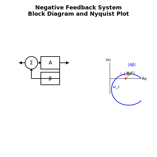
The stability of a negative feedback system is determined by the loop gain Aβ and its phase margin. The Nyquist criterion states that if the plot of Aβ(jω) encircles the point (−1, 0) in the complex plane, the system is unstable. The phase margin, defined as:
where ωc is the crossover frequency, must be positive for stability. Practical systems often require a phase margin > 45° to avoid oscillatory transients.
Real-World Applications
Negative feedback is ubiquitous in control systems, such as:
- Operational Amplifiers: Precision voltage amplification with bandwidth extension.
- Power Supplies: Voltage regulation via feedback loops comparing output to a reference.
- Automotive Cruise Control: Speed adjustments based on feedback from wheel sensors.
Mathematical Derivation of Sensitivity Reduction
The sensitivity of the closed-loop gain Af to variations in open-loop gain A is given by:
This shows that negative feedback reduces sensitivity to component variations by a factor of (1 + Aβ), enhancing robustness in industrial automation systems where component tolerances vary.
Case Study: PID Controllers
Proportional-Integral-Derivative (PID) controllers leverage negative feedback to minimize error e(t) between a desired setpoint and measured output. The control law:
is implemented with feedback to adjust system dynamics dynamically. Tuning Kp, Ki, and Kd optimizes response time and overshoot, critical in robotics and process control.
6. Key Textbooks on Feedback Systems
6.1 Key Textbooks on Feedback Systems
- Feedback Systems: An Introduction for Scientists and Engineers, Second ... — Description The essential introduction to the principles and applications of feedback systems―now fully revised and expandedThis textbook covers the mathematics needed to model, analyze, and design feedback systems. Now more user-friendly than ever, this revised and expanded edition of Feedback Systems is a one-volume resource for students and researchers in mathematics and engineering. It ...
- PDF Nonlinear Systems and Control Lecture # 16 Feedback Systems: Passivity ... — Theorem 6.3: Consider the feedback connection of two dynamical systems. When u = 0, the origin of the closed-loop system is asymptotically stable if each feedback component is either
- Design of Feedback Control Systems 4th Ed - Stefani PDF - Scribd — Raymond T. Stefani, 4th ed., Oxford series in electrical and computer engineering. No part of this publication may be reproduced without the prior permission of Oxford University Press. The feedback concept 1.2. Modeling System Dynamics Electrical Components 1.3. Mesh Analysis 1.3. State Variables 1.4. Node Analysis 1.4. Analogies 1.7. Gear Trains and Transformers 1.8.
- PDF Feedback Systems — The book is designed for use in a 10- to 15-week course in feedback systems that provides many of the key concepts needed in a variety of disciplines. For a 10-week course, Chapters 1-2, 4-6 and 8-11 can each be covered in a week's time, with the omission of some topics from the final chapters.
- PDF Feedback Systems: An Introduction for Scientists and Engineers — Preface This book provides an introduction to the basic principles and tools for design and analysis of feedback systems. It is intended to serve a diverse audience of scientists and engineers who are interested in understanding and utilizing feedback in physical, biological, information, and economic systems.
- Feedback Systems | Princeton University Press — This textbook covers the mathematics needed to model, analyze, and design feedback systems. Now more user-friendly than ever, this revised and expanded edition of Feedback Systems is a one-volume resource for students and researchers in mathematics and engineering.
- PDF ECE 380: Control Systems - Purdue University — Acknowledgments Parts of these course notes are loosely based on lecture notes by Professors Daniel Liberzon, Sean Meyn, and Mark Spong (University of Illinois), on notes by Professors Daniel Davison and Daniel Miller (University of Waterloo), and on parts of the textbook Feedback Control of Dynamic Systems (5th edition) by Franklin, Powell and Emami-Naeini. I claim credit for all typos and ...
- Feedback Systems Textbook: Control Theory for Engineers — Textbook on feedback systems, control theory, and engineering for scientists and engineers. Includes models, analysis, and design techniques.
- Feedback Systems: An Introduction for Scientists and Engineers — This book provides an introduction to the mathematics needed to model, analyze, and design feedback systems. It is an ideal textbook for undergraduate and graduate students, and is indispensable ...
6.2 Research Papers and Articles
- The Sunny Side of Negative Feedback: Negative Feedback Enhances One's ... — Fourth, recent research suggests that there may be individual difference in handling negative feedback and one's feedback control system would impact the coping style following negative feedback (Franklin and Frank, 2015). It is a promising issue to explore the individual factors that may modulate the intertemporal effect of negative feedback ...
- Cyclic Negative Feedback Systems: What is the Chance of ... - Springer — Many biological oscillators have a cyclic structure consisting of negative feedback loops. In this paper, we analyze the impact that the addition of a positive or a negative self-feedback loop has on the oscillatory behavior of the three negative feedback oscillators proposed by Tsai et al. (Science 231:126-129, 2008) where, in contrast with numerous oscillator models, the interactions ...
- The future of feedback: Motivating performance improvement through ... — However, when the feedback was negative, recipients judged the failures as due principally to causes beyond their control, such as task demands and bad luck. They did not accept the negative feedback received, judging it as less accurate (t(192) = 7.50, p < .001) and judging the feedback provider less qualified to give it t(192) = 5.25, p ...
- 29 Negative feedback - Oxford Academic — Negative feedback is an essential constituent of any control system. It is illustrated for the case of an electronic voltage amplifier. ... In the context of an electronic amplifier, negative feedback is applied with two aims in mind: ... A block diagram of a generic negative-feedback system is shown in Fig. 29.1.
- PDF Cyclic negative feedback systems: what is the chance of ... - Inria — In this paper, we study the cyclic inhibitory feedback systems considered by Tsai et al. (2008) where the symmetry of the cycle can be broken by an addi-tional negative or positive self-feedback loop. In Sect. 2 we present the models. In Sect. 3.1 we discuss the nature of the interactions and in Sect. 3.2 we ex-
- Negative Feedback System as Optimizer for Machine Learning Systems — the inverse of a linear or non-linear function that is in the feedback path. This property of negative feedback systems has been widely used in analog electronic circuits to construct precise closed-loop functions. This paper describes how the function-inverting process of a negative feedback system serves as a physical
- Negative Feedback System - an overview | ScienceDirect Topics — Alternatively, to implement negative feedback on the transcriptional or translational level, a recent study used a de novo-designed protein pair to realize post-translational negative feedback [37]. Negative feedback circuits have also been used to address issues that arise from competition for limited and shared cellular resources.
- A feedback control principle common to several biological and ... — The behaviour of discrete-event feedback systems is determined by how a control variable changes upon receipt of positive or negative feedback. The most common first-order response to feedback can be described as additive, in which a constant is added or subtracted to the variable, or multiplicative, where the variable is multiplied or divided ...
- PDF Feedback Systems - Caltech Computing — 6-2 CHAPTER 6. LINEAR SYSTEMS For other systems, nonlinearities cannot be ignored, espec ially if one cares about the global behavior of the system. The predator-prey problem is one exam-ple of this: to capture the oscillatory behavior of the interdependent populations we must include the nonlinear coupling terms. Other examplesincludeswitch-
- PDF NEGATIVE FEEDBACK - Springer — Negative feedback has best accuracy, because an accurately reduced copy of the output signal is compared with the original input signal. Any deviation ... A better model for describing electronic feedback systems is the asymptotic-gain model. The starting point to come to the asymptotic-gain model is the superposition model, shown in figure 3.1 ...
6.3 Online Resources and Tutorials
- PDF Nonlinear Systems and Control Lecture # 16 Feedback Systems: Passivity ... — Theorem 6.1: The feedback connection of two passive systems is passive Theorem 6.3: Consider the feedback connection of two dynamical systems. When u= 0, the origin of the closed-loop system is asymptotically stable if each feedback component is either strictly passive, or output strictly passive and zero-state observable
- Readings | Analysis and Design of Feedback Control Systems | Mechanical ... — [JKR] Chapter 2: Properties and Modeling of Feedback Systems. 2.3.2 Effect of Feedback on Nonlinearities (PDF - 1.6MB) Lec 15-16 [JKR] Chapter 3: Linear System Response. 3.5 Relationships Between Transient Response and Frequency Response (PDF - 1.8MB) Lec 17-18 [FPE] Chapter 7: State-Space Design. 7.1 Advantages of State-Space
- 6.4 Negative Feedback Amplifier - Applied Electrical ... - UMass — 6.4 Negative Feedback Amplifier Op amp circuits can achieve controlled voltage gain while avoiding saturation by employing negative feedback.The basic idea is to provide a path between the op amp output node, which has voltage V o, and the inverting terminal input node, which has voltage V -.In the example circuit shown in figure 6.22, this is accomplished via the feedback resistor R f.
- PDF Electronic Feedback Systems: Lecture 17 - opencw.aprende.org — 17-4 Electronic Feedback Systems Viewgraph 17.3 950 Hz, a = 24 390 H_ a = 2.7 Viewgraph 17.4 Bode Plot for a = 80 Magnitude S1 ... crossover frequency to a region of negative phase margin. Describing-function analysis indicates the potential for this type of behavior, predicts oscillation parameters in systems where ...
- PDF Feedback Systems - Caltech Computing — to nonlinear systems, frequency domain analysis applies primarily to linear systems. The notions of gain and phase can, however, be generalized to nonlinear systems and, in particular, propagation of sinusoidal signals through a nonlinear system can approximately be captured by an analog of the frequency response called the describing function.
- Resources | Signals and Systems - MIT OpenCourseWare — Learning Resource Types. theaters Lecture Videos. assignment_turned_in Problem Sets with Solutions. ... Continuous-time feedback and control, part 1 Lecture 13: Continuous-Time (CT) Feedback and Control, Part 2 ... MIT OpenCourseWare is an online publication of materials from over 2,500 MIT courses, freely sharing knowledge with learners and ...
- PDF 7.5 Frequency-dependent Feedback - University of Oregon — the inverting and the non-inverting configurations. In this section we will discuss negative feedback in a very general way, followed by some examples illustrating how negative feedback can be used to improve performance. 7.6.1 Gain Consider the rather abstract schematic of a negative feedback amplifier system shown in Fig. 44.
- PDF Feedback Systems - Caltech Computing — In many cases, we create systems with a linear input/output response through the use of feedback. Indeed, it was the desire for linear behavior that led Harold S. Black to the invention of the negative feedback amplifier. Almost all modern signal processing systems, whether analog or digital, use feedback to produce lin-
- Feedback Systems: An Introduction for Scientists and Engineers — Feedback Systems is a complete one-volume resource for students and researchers in mathematics, engineering, and the sciences. Discover the world's research 25+ million members
- PDF 16.30 Topic 3: Frequency response methods - MIT OpenCourseWare — • Phase Margin: angle by which the system phase differs from 180 when the loop gain is 1. • Let ω c be the frequency at which |L(jω c)| = 1, and φ = L(jω c) (typically less than zero), then PM = 180 + φ • Typical stable system needs both GM > 0 and PM > 0 Fig. 5: Gain and Phase Margin for stable system in a polar plot