Definition and Role of Passive Components

Passive components—resistors, capacitors, and inductors—are fundamental elements in AC circuits, characterized by their inability to introduce energy amplification. Unlike active components (e.g., transistors or op-amps), they do not require an external power source to function. Instead, they modify voltage and current through energy storage (capacitors, inductors) or dissipation (resistors). Their behavior in AC circuits is governed by frequency-dependent impedance rather than simple resistance.

Impedance and Frequency Response

The impedance Z of a passive component in an AC circuit is a complex quantity, combining resistance R and reactance X:

For resistors, X = 0, making impedance purely real. Capacitors and inductors introduce reactance:

• Capacitive reactance (X_C): Decreases with frequency, given by X_C = 1/(ωC), where ω = 2πf.
• Inductive reactance (X_L): Increases with frequency, expressed as X_L = ωL.

Phase Relationships

Passive components introduce phase shifts between voltage and current:

• Resistors: Voltage and current remain in phase (θ = 0°).
• Capacitors: Current leads voltage by 90° (θ = -90°).
• Inductors: Voltage leads current by 90° (θ = +90°).

These phase relationships are critical in power factor correction, filter design, and impedance matching.

Energy Dynamics

Capacitors and inductors store energy in electric and magnetic fields, respectively, leading to transient responses in AC circuits. The energy stored in a capacitor (E_C) and inductor (E_L) is:

Resistors dissipate energy as heat, with power loss given by P = I²R.

Practical Applications

Passive components are ubiquitous in:

• Filters: High-pass, low-pass, and band-pass configurations rely on LC or RC networks.
• Resonant circuits: Tank circuits (parallel LC) exploit reactance cancellation at resonant frequency.
• Power systems: Capacitors compensate for inductive loads to improve power factor.

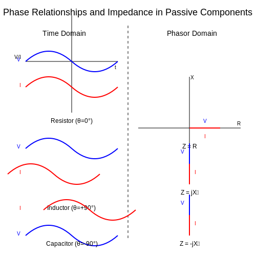
Key Characteristics in AC vs DC Circuits

Impedance vs Resistance

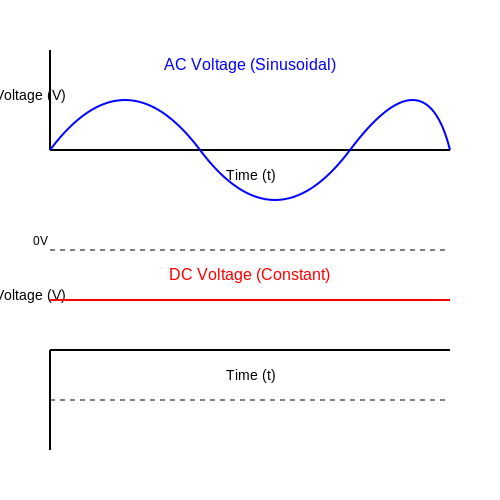
In DC circuits, passive components exhibit purely resistive behavior, where opposition to current flow is described by resistance R. However, in AC circuits, the concept of impedance (Z) becomes critical, encompassing both resistance and reactance (X). The impedance of a component is frequency-dependent and is given by:

For inductors, reactance is X_L = ωL = 2πfL, while for capacitors, it is X_C = 1/(ωC) = 1/(2πfC). Unlike DC, where components behave statically, AC circuits introduce phase shifts between voltage and current due to reactance.

Phase Relationships

In purely resistive AC circuits, voltage and current remain in phase. However, inductors cause current to lag voltage by 90° (π/2 radians), while capacitors cause current to lead voltage by 90°. This phase difference is represented in the complex plane, where impedance is a vector combining resistive (real) and reactive (imaginary) components.

Power Dissipation

In DC circuits, power dissipation is straightforward: P = VI = I²R = V²/R. In AC circuits, power becomes complex due to phase differences. The real power (P) dissipated in resistors is:

where cos(θ) is the power factor. Inductors and capacitors store and release energy, contributing to reactive power (Q = VI sin(θ)), which does no net work but affects system efficiency.

Frequency Dependence

DC analysis assumes zero frequency, rendering reactive components (inductors as short circuits, capacitors as open circuits at steady state). In AC, frequency (f) dictates component behavior:

• Inductors block high frequencies (X_L ∝ f).
• Capacitors block low frequencies (X_C ∝ 1/f).

This property is exploited in filters, where passive components shape frequency response. For example, a low-pass RC filter attenuates signals above its cutoff frequency:

Transient vs Steady-State Response

DC circuits reach steady-state instantaneously (ignoring parasitic effects). AC circuits exhibit transient behavior during startup or switching, where energy storage in inductors and capacitors causes oscillations or damped responses. The time constant τ = L/R or τ = RC governs this transient phase.

Practical Implications

In power distribution, AC’s ability to transform voltages via transformers (relying on inductive coupling) makes it preferable over DC for long-distance transmission. However, DC is dominant in electronic devices where stable voltage rails are required. Understanding these differences is crucial for designing circuits like:

• AC-DC converters (rectifiers with smoothing capacitors).
• Resonant circuits (tank circuits using LC combinations).
• Impedance matching networks (maximizing power transfer).

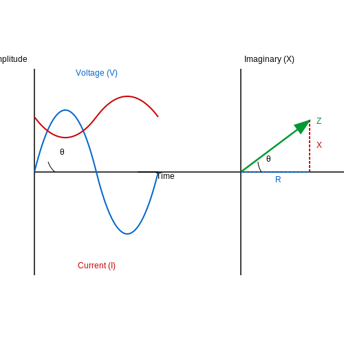
1.3 Phasor Representation and Impedance

In AC circuit analysis, phasors provide a powerful mathematical tool to simplify the treatment of sinusoidal signals. A phasor is a complex number representing the amplitude and phase of a sinusoid, typically expressed in exponential form:

where V_m is the peak voltage magnitude and φ is the phase angle. This representation allows us to convert differential equations describing AC circuits into algebraic equations in the complex domain.

Phasor Transformation of Circuit Elements

The behavior of passive components in the phasor domain is characterized by their impedance Z, defined as the ratio of voltage phasor to current phasor:

For the three fundamental passive components:

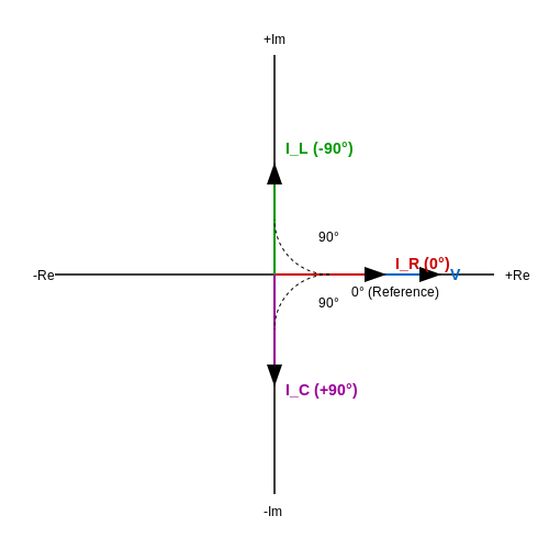
• Resistor (R): Pure real impedance Z_R = R, with voltage and current in phase.
• Inductor (L): Purely imaginary impedance Z_L = jωL, where current lags voltage by 90°.
• Capacitor (C): Purely imaginary impedance Z_C = 1/(jωC), where current leads voltage by 90°.

Complex Impedance and Admittance

The generalized impedance Z can be expressed in rectangular or polar form:

where R is resistance, X is reactance, and θ = tan^-1(X/R). The reciprocal of impedance is admittance Y:

with conductance G and susceptance B.

Kirchhoff's Laws in Phasor Form

All DC circuit analysis techniques extend to AC circuits using phasors:

• KVL: The sum of voltage phasors around any closed loop equals zero.
• KCL: The sum of current phasors entering any node equals zero.

This allows application of nodal analysis, mesh analysis, and network theorems to AC circuits by replacing resistances with complex impedances.

Power in Phasor Domain

Complex power S combines real (active) power P and reactive power Q:

where I* is the complex conjugate of current. The power factor is given by:

Practical Applications

Phasor analysis is essential for:

• Power system load flow studies
• Filter design and frequency response analysis
• Impedance matching in RF circuits
• Three-phase power calculations

The following diagram illustrates the phase relationships between voltage and current for R, L, and C components:

Behavior Under Alternating Current

Impedance and Phase Relationships

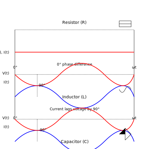
In AC circuits, passive components exhibit frequency-dependent behavior due to their inherent reactance. The total opposition to current flow, known as impedance (Z), combines resistance (R) and reactance (X). For a sinusoidal voltage V(t) = V₀sin(ωt), the current response depends on the component type:

where j represents the imaginary unit (√-1). The phase difference (θ) between voltage and current arises from reactive effects:

Resistors in AC Circuits

Resistors maintain a linear voltage-current relationship regardless of frequency. For V(t) = V₀sin(ωt), Ohm's law gives:

The instantaneous power dissipation oscillates at twice the source frequency:

Inductors in AC Circuits

Inductors oppose current changes via back-EMF, introducing a 90° phase lag. The inductive reactance (X_L) scales linearly with frequency:

Current lags voltage by π/2 radians:

Capacitors in AC Circuits

Capacitors exhibit frequency-dependent conductive behavior, with current leading voltage by 90°. The capacitive reactance (X_C) varies inversely with frequency:

The current response becomes:

Power Dissipation and Quality Factor

Reactive elements store and release energy, causing apparent power (S = VI) to exceed real power (P = VIcosθ). The quality factor (Q) quantifies energy storage efficiency:

For series RLC circuits, this reduces to:

2.2 Power Dissipation and RMS Values

In AC circuits, power dissipation differs fundamentally from DC due to the time-varying nature of voltage and current. For a sinusoidal voltage v(t) = V_psin(ωt) and current i(t) = I_psin(ωt + θ), the instantaneous power is:

Using the trigonometric identity for product of sines, this expands to:

The first term represents the real power (average power dissipated), while the second term oscillates at twice the frequency, contributing no net energy over a full cycle. Integrating over one period T = 2π/ω yields the average power:

Root-Mean-Square (RMS) Values

RMS values provide an equivalent DC measure for AC quantities. For a periodic function f(t) with period T, the RMS value is defined as:

For a sinusoidal current i(t) = I_psin(ωt), the RMS value becomes:

Similarly, the RMS voltage is V_RMS = V_p/√2. Power dissipation in resistive elements can then be expressed in familiar DC-like forms:

Power Factor and Reactive Components

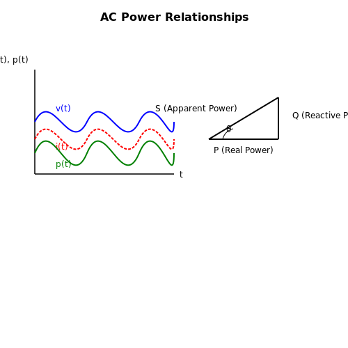
The cos(θ) term in the power equation is the power factor, representing the phase shift between voltage and current. In purely resistive loads, θ = 0 and all power is dissipated as heat. With reactive components (inductors/capacitors):

• Real power (P): V_RMSI_RMScos(θ) (measured in watts)
• Reactive power (Q): V_RMSI_RMSsin(θ) (measured in VAR)
• Apparent power (S): V_RMSI_RMS (measured in VA)

These relationships form the power triangle, where S² = P² + Q². In industrial systems, low power factors due to inductive loads (e.g., motors) necessitate corrective capacitors to minimize reactive power and reduce line losses.

2.3 Practical Applications and Limitations

Resistors in AC Circuits

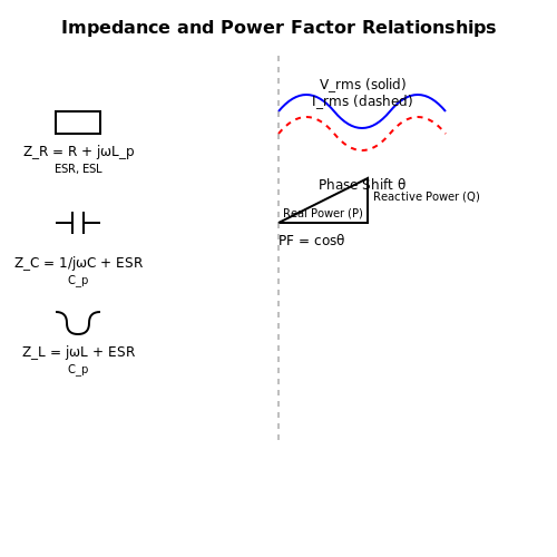
Resistors exhibit minimal frequency-dependent behavior in AC circuits, making them ideal for current-limiting and voltage-divider applications. However, parasitic inductance (L_p) and capacitance (C_p) become significant at high frequencies (f > 10 MHz). The impedance of a non-ideal resistor is given by:

In precision measurement circuits, thermal noise (Johnson-Nyquist noise) becomes a limiting factor:

Capacitors in AC Applications

Capacitors are widely used for filtering, coupling, and energy storage. The effective impedance includes equivalent series resistance (ESR) and inductance (ESL):

Key limitations include:

• Dielectric absorption: Causes voltage retention after discharge, critical in sample-and-hold circuits.
• Temperature dependence: Ceramic capacitors exhibit strong capacitance shifts with temperature (e.g., X7R, Y5V dielectrics).
• Voltage coefficient: Capacitance decreases with applied DC bias in multilayer ceramics.

Inductors in AC Systems

Inductors are essential in power supplies (DC-DC converters) and RF matching networks. Practical limitations include:

Where R_AC accounts for skin and proximity effects. Core losses (P_core) in magnetic materials follow Steinmetz's equation:

Passive Component Selection Criteria

For high-frequency designs (>100 MHz), component packaging dominates performance:

• Resistors: Thin-film outperforms thick-film due to lower parasitics.
• Capacitors: NP0/C0G dielectrics provide stable capacitance, while tantalum capacitors exhibit low ESL.
• Inductors: Air-core or powdered-iron cores minimize hysteresis losses.

Case Study: Power Factor Correction

In AC-DC converters, passive components correct phase differences between voltage and current. The power factor (PF) is given by:

Where θ is the phase angle. A practical PFC circuit combines:

• Boost inductor (100 μH–1 mH) to shape input current
• DC-link capacitor (100–470 μF) to smooth output voltage
• Snubber networks (RC) to suppress switching transients

Inductive Reactance and Frequency Dependence

Fundamentals of Inductive Reactance

In an AC circuit, an inductor opposes changes in current by inducing a back-EMF proportional to the rate of current change. This opposition is quantified as inductive reactance (X_L), which depends on both the inductance (L) and the angular frequency (ω) of the AC signal. Unlike resistance, reactance does not dissipate energy but stores it temporarily in the magnetic field.

The relationship between voltage and current in an ideal inductor is given by Faraday’s law:

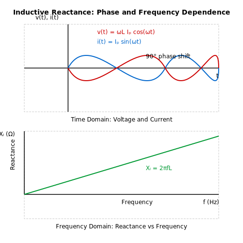
For a sinusoidal current i(t) = I_p sin(ωt), the voltage leads the current by 90°:

Derivation of Inductive Reactance

Using phasor analysis, the impedance of an inductor is purely reactive:

where j is the imaginary unit. The magnitude of this impedance defines the inductive reactance:

Here, f is the frequency in hertz. This linear dependence on frequency implies that inductors behave as short circuits at DC (f = 0) and increasingly oppose current as frequency rises.

Frequency Response and Practical Implications

The frequency dependence of X_L has critical applications:

• Filters: Inductors are used in low-pass and band-pass filters to block high-frequency signals.
• Impedance Matching: In RF circuits, inductive reactance compensates for capacitive effects to maximize power transfer.
• Resonant Circuits: Combined with capacitors, inductors form LC tanks where X_L = X_C at resonance.

For example, a 10 mH inductor exhibits X_L ≈ 6.28 Ω at 100 Hz but 6.28 kΩ at 100 kHz. This property is exploited in noise suppression and signal tuning.

Non-Ideal Behavior and Parasitic Effects

Real inductors exhibit:

• Resistive Losses: Winding resistance (R_DC) causes power dissipation, modeled as a series resistor.
• Capacitance: Inter-winding capacitance creates a self-resonant frequency beyond which the inductor behaves as a capacitor.
• Core Losses: Magnetic hysteresis and eddy currents in ferromagnetic cores reduce efficiency at high frequencies.

The quality factor (Q) quantifies these losses:

where R_s is the equivalent series resistance. High-Q inductors are essential in oscillators and tuned amplifiers.

Historical Context

Inductive reactance was first systematically analyzed by Oliver Heaviside in the 1880s as part of his work on AC transmission lines. His reformulation of Maxwell’s equations into modern impedance concepts laid the groundwork for RF engineering.

Phase Relationships in Inductive Circuits

In an AC circuit containing purely inductive elements, the phase relationship between voltage and current is fundamentally different from resistive circuits. The voltage across an inductor leads the current through it by 90° (π/2 radians). This phase shift arises due to Faraday's law of induction, where the induced electromotive force (EMF) opposes the change in current.

Mathematical Derivation of Phase Shift

Consider an ideal inductor with inductance L connected to an AC voltage source v(t) = V_msin(ωt). The relationship between voltage and current in an inductor is given by:

Solving for the current i(t):

This clearly shows the current lags the voltage by 90°. The quantity ωL represents the inductive reactance X_L, with units of ohms.

Phasor Representation

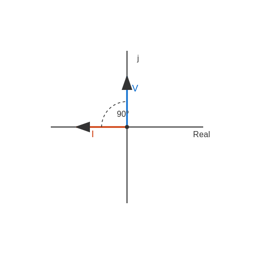
The phase relationship is best visualized using phasor diagrams. In the complex plane:

• The voltage phasor points along the positive imaginary axis
• The current phasor points along the negative real axis
• The angle between them is always 90° with voltage leading

Power Considerations

The instantaneous power in an inductive circuit is:

Using trigonometric identities, this becomes:

This shows that:

• The average power over a cycle is zero - inductors don't dissipate energy
• Power oscillates between the source and magnetic field at twice the source frequency

Practical Implications

In real-world applications, this phase shift has significant consequences:

• Power factor correction: Industrial loads with inductive components require capacitors to offset lagging currents
• Transformer operation: Magnetizing current lards voltage by nearly 90° in unloaded transformers
• Motor starting currents: Induction motors draw lagging currents that can be 5-6 times the running current

Non-Ideal Inductors

Real inductors have resistive components, modifying the phase relationship. The impedance becomes:

The phase angle θ between voltage and current is then:

This results in:

• Current still lags voltage, but by less than 90°
• Power dissipation occurs in the resistive component
• The quality factor Q = ωL/R determines how close the inductor is to ideal

3.3 Energy Storage and Magnetic Fields

In AC circuits, inductors and capacitors store energy in magnetic and electric fields, respectively. The dynamics of energy storage and release govern the transient and steady-state behavior of these circuits, particularly in resonant systems and power applications.

Energy Stored in an Inductor

The energy W_L stored in the magnetic field of an inductor with inductance L carrying a current i(t) is given by:

For a sinusoidal current i(t) = I_p sin(ωt), the instantaneous energy oscillates between zero and a maximum value:

The average energy stored over one cycle is:

where I_rms is the root-mean-square current. This expression highlights the dependence of stored energy on both inductance and the square of the current.

Magnetic Field Energy Density

The energy stored in a magnetic field can also be expressed in terms of the magnetic flux density B and the magnetic field intensity H. For a linear, isotropic medium, the energy density u_m is:

where μ is the permeability of the medium. Integrating this over the volume of the magnetic field yields the total stored energy:

Practical Implications in AC Circuits

In power systems, the energy storage capability of inductors affects:

• Reactive power management: Inductive loads require reactive power to sustain magnetic fields, leading to phase shifts between voltage and current.
• Transient response: The time constant τ = L/R governs how quickly an inductive circuit reaches steady state after a disturbance.
• Resonance phenomena: In LC circuits, energy oscillates between the inductor’s magnetic field and the capacitor’s electric field at the resonant frequency f_r = 1/(2π√LC).

Core Losses and Hysteresis

In real inductors with ferromagnetic cores, energy losses occur due to:

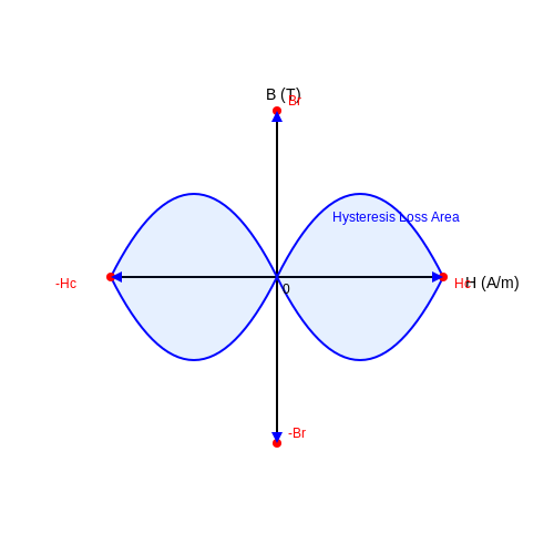
• Hysteresis losses: Energy dissipated as the magnetic domains realign with the alternating field, proportional to the area of the B-H loop.
• Eddy currents: Circulating currents induced in the core material, minimized by laminating the core or using powdered iron.

The total power loss P_core in a magnetic core is empirically modeled by the Steinmetz equation:

where k_h and k_e are hysteresis and eddy current coefficients, and α (typically 1.6–2.0) depends on the material.

Mutual Inductance and Coupled Energy

When two inductors are magnetically coupled, their mutual inductance M influences the total stored energy. For two coils with currents i₁ and i₂:

The sign of the mutual term depends on the relative winding directions. This principle underpins transformers, where energy transfers between primary and secondary windings via the shared magnetic flux.

4.1 Capacitive Reactance and Frequency Response

In an AC circuit, a capacitor does not behave like a simple resistor. Instead, its opposition to current flow is frequency-dependent and characterized by capacitive reactance (X_C). Unlike resistance, reactance does not dissipate energy but temporarily stores it in the electric field between the capacitor plates.

Derivation of Capacitive Reactance

The current through a capacitor is proportional to the rate of change of voltage across it:

For a sinusoidal voltage source v(t) = V_msin(ωt), the current becomes:

The amplitude of the current is I_m = ωCV_m, so the ratio of voltage amplitude to current amplitude defines the reactance:

This shows that capacitive reactance is inversely proportional to both frequency (f) and capacitance (C).

Frequency Response of a Capacitor

The impedance of a capacitor in the complex plane is purely imaginary:

At low frequencies, X_C becomes very large, effectively blocking DC signals. At high frequencies, X_C approaches zero, allowing AC signals to pass with minimal opposition. This property makes capacitors essential in:

• Coupling circuits (blocking DC while passing AC)
• Filter design (low-pass, high-pass, and band-pass configurations)
• Noise suppression (bypassing high-frequency interference to ground)

Phase Relationship in Capacitive Circuits

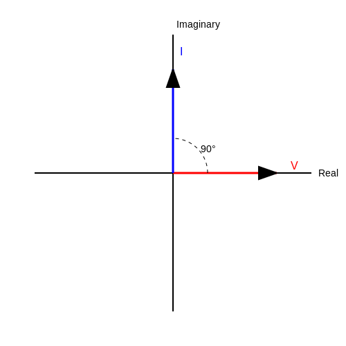
In a purely capacitive circuit, the current leads the voltage by 90°. This phase shift arises because the current depends on the rate of change of voltage rather than its instantaneous value. The phasor representation illustrates this relationship:

Practical Implications

In real-world applications, parasitic effects such as equivalent series resistance (ESR) and inductance (ESL) modify the ideal behavior of capacitors. For instance, at very high frequencies, ESL dominates, causing the impedance to rise again. This non-ideal response is critical in:

• Power supply decoupling (selecting capacitors with low ESR for effective filtering)
• RF circuit design (minimizing ESL to maintain low impedance at GHz frequencies)
• Signal integrity analysis (modeling capacitors as RLC networks in high-speed PCBs)

4.2 Phase Shift in Capacitive Circuits

Fundamental Behavior of Capacitors in AC Circuits

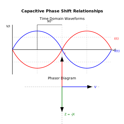
In an AC circuit, a capacitor opposes changes in voltage by drawing or supplying current proportional to the rate of voltage change. Unlike resistors, capacitors introduce a phase shift between voltage and current. The current leads the voltage by 90° (π/2 radians) in an ideal capacitor, a consequence of the derivative relationship between voltage and current:

For a sinusoidal voltage \( V(t) = V_0 \sin(\omega t) \), the current becomes:

This results in a current waveform \( I(t) = I_0 \cos(\omega t) \), where \( I_0 = \omega C V_0 \), confirming the 90° lead.

Impedance and Phase Angle

The capacitive reactance (\( X_C \)) quantifies the opposition to AC current and is frequency-dependent:

In phasor notation, the impedance of a capacitor is purely imaginary:

The negative imaginary component reflects the 90° phase shift. When combined with resistive elements, the total impedance (\( Z \)) determines the circuit's phase angle (\( \theta \)):

Practical Implications

Phase shifts in capacitive circuits are critical in:

• Power factor correction: Capacitors counteract inductive lag in AC power systems.
• Filter design: High-pass and low-pass filters exploit phase shifts to attenuate specific frequencies.
• Oscillators and timing circuits: RC networks generate controlled phase delays for signal processing.

Visualizing Phase Relationships

A phasor diagram illustrates the 90° lead of current over voltage. The voltage phasor (\( V \)) lags behind the current phasor (\( I \)), while the impedance phasor (\( Z \)) points downward in the complex plane due to the negative reactance.

Real-World Non-Ideal Effects

Practical capacitors exhibit parasitic resistance (equivalent series resistance, ESR) and inductance (ESL), modifying the phase shift. At high frequencies, ESL dominates, causing the phase angle to deviate from -90° and even become positive (inductive behavior).

4.3 Energy Storage and Electric Fields

Electric Field Energy in Capacitors

In AC circuits, capacitors store energy in the form of an electric field established between their plates. The instantaneous energy E_C stored in a capacitor with capacitance C and voltage v(t) is given by:

For a sinusoidal voltage v(t) = V_p sin(ωt), the energy oscillates between zero and a maximum value E_max = ½ C V_p². The energy transfer rate, or reactive power Q, quantifies the cyclic storage and release of energy without net dissipation.

Derivation of Reactive Power in Capacitors

The current through a capacitor leads the voltage by 90° (i(t) = ωC V_p cos(ωt)). The instantaneous power p(t) = v(t) i(t) becomes:

This oscillates at twice the source frequency, with an amplitude equal to the reactive power Q = ωC V_rms², where V_rms = V_p/√2.

Practical Implications

In power systems, capacitor banks are deployed for reactive power compensation to improve grid efficiency. For example, industrial loads with inductive characteristics (e.g., motors) cause lagging power factors; capacitors supply leading reactive power to offset this, reducing apparent power demands.

Energy Density in Dielectric Materials

The energy storage capacity of a capacitor is influenced by the dielectric material’s permittivity ε = ε₀ε_r. The volumetric energy density u_E within the electric field E is:

High-permittivity ceramics (e.g., barium titanate) enable compact high-energy capacitors, critical for pulsed-power applications.

Frequency Dependence and Losses

At high frequencies, dielectric losses manifest as a complex permittivity ε = ε′ − jε″, where ε″ represents energy dissipation. The loss tangent tan δ = ε″/ε′ determines the capacitor’s quality factor Q = 1/tan δ.

For instance, polypropylene capacitors exhibit tan δ ≈ 0.0002 at 1 kHz, making them suitable for precision AC applications, while electrolytics (tan δ ≈ 0.1) are restricted to low-frequency filtering.

Series and Parallel RLC Circuits

Impedance in Series RLC Circuits

In a series RLC circuit, the total impedance Z is the phasor sum of resistance R, inductive reactance X_L, and capacitive reactance X_C. The general form is:

The magnitude of impedance follows from the Pythagorean theorem:

At resonance (X_L = X_C), the circuit becomes purely resistive, with minimum impedance and maximum current. The resonant frequency f₀ is:

Admittance in Parallel RLC Circuits

For parallel configurations, admittance Y (inverse of impedance) is the sum of conductances and susceptances:

The magnitude of admittance is:

At resonance, the imaginary component cancels out, leaving only the conductive term. The resonant frequency remains identical to the series case.

Quality Factor and Bandwidth

The quality factor Q quantifies frequency selectivity. For series RLC:

For parallel RLC:

The bandwidth BW (difference between upper and lower -3dB frequencies) relates to Q as:

Practical Applications

• RF Filters: Series/parallel RLC networks form bandpass/bandstop filters in communication systems.
• Impedance Matching: Used in antenna systems to maximize power transfer.
• Oscillators: LC tank circuits generate stable frequencies in clock circuits.

Transient Response Analysis

The step response of an RLC circuit is governed by a second-order differential equation:

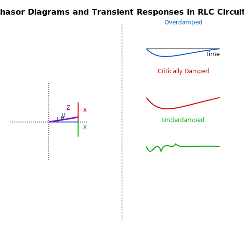
where α is the damping coefficient (α = R/2L for series, α = 1/2RC for parallel). Solutions fall into three regimes:

• Overdamped (α > ω₀): Non-oscillatory decay
• Critically damped (α = ω₀): Fastest settling without oscillation
• Underdamped (α < ω₀): Damped sinusoidal response

Resonance Phenomena and Bandwidth

Series and Parallel Resonance

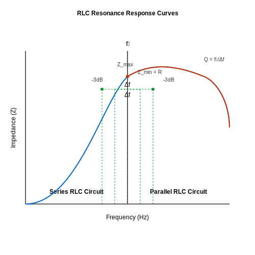
In AC circuits containing inductors and capacitors, resonance occurs when the reactive components cancel each other out, resulting in a purely resistive impedance. For a series RLC circuit, the resonant frequency f_r is given by:

At resonance, the impedance Z is minimized (Z = R), and the current reaches its peak. In parallel RLC circuits, resonance also occurs at the same frequency, but the impedance is maximized instead.

Quality Factor (Q) and Bandwidth

The sharpness of the resonance peak is quantified by the quality factor Q, defined as the ratio of resonant frequency to bandwidth:

where Δf is the bandwidth—the frequency range between the two half-power (-3 dB) points. For a series RLC circuit, Q can also be expressed in terms of circuit parameters:

Practical Implications of Resonance

Resonance is exploited in applications such as:

• Tuned circuits in radio receivers, where selectivity is determined by Q.
• Impedance matching networks to maximize power transfer.
• Filter design, where high-Q circuits provide steeper roll-offs.

Mathematical Derivation of Bandwidth

The bandwidth Δf is derived from the frequencies where the power dissipated in the resistor is half of its maximum value. For a series RLC circuit:

where f₁ and f₂ are the lower and upper cutoff frequencies, respectively. This relationship shows that higher Q (lower R or higher L/C) results in a narrower bandwidth.

Effect of Damping on Resonance

Damping, introduced by resistance, affects the resonance peak. Underdamped circuits (Q > 0.5) exhibit a pronounced peak, while critically damped (Q = 0.5) and overdamped (Q < 0.5) circuits show a flattened response. The damping ratio ζ is related to Q by:

Real-World Considerations

In practical circuits, component non-idealities (e.g., inductor resistance, capacitor ESR) affect resonance. For instance, the effective Q of an inductor is given by:

where R_coil is the winding resistance. High-frequency effects like skin depth and parasitic capacitance further influence performance.

5.3 Filter Applications and Design Considerations

Frequency Response and Transfer Functions

The behavior of passive filters in AC circuits is governed by their frequency response, which describes how the output amplitude and phase vary with input frequency. For a generic RLC network, the transfer function H(ω) is derived from the impedance divider rule:

where Z₁ and Z₂ are complex impedances. For a first-order RC low-pass filter, this reduces to:

The cutoff frequency (ω_c) occurs when the magnitude falls to 1/√2 of its maximum value:

Filter Topologies and Their Trade-offs

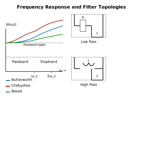
Passive filters are categorized by their response characteristics:

• Butterworth: Maximally flat passband, but slower roll-off.
• Chebyshev: Steeper roll-off at the expense of passband ripple.
• Bessel: Linear phase response, ideal for preserving signal shape.

The choice of topology depends on the application. For instance, audio systems prioritize phase linearity (Bessel), while RF applications may favor sharp transitions (Chebyshev).

Quality Factor (Q) and Bandwidth

For resonant circuits (e.g., bandpass filters), the quality factor Q determines selectivity:

where ω₀ is the resonant frequency and Δω is the bandwidth. High-Q circuits exhibit narrow bandwidths, critical in applications like tuners or interference rejection.

Component Non-Idealities

Real-world components introduce deviations from theoretical models:

• Parasitic capacitance/inductance: Alters high-frequency response.
• Resistor tolerance: Affects cutoff frequency accuracy.
• Temperature drift: Impacts stability in precision filters.

For example, a ceramic capacitor’s effective capacitance may drop at high frequencies due to parasitic inductance.

Design Methodology

A systematic approach to filter design involves:

1. Specification: Define passband ripple, stopband attenuation, and transition width.
2. Prototype selection: Choose a normalized low-pass filter (e.g., 1 rad/s cutoff).
3. Scaling: Transform component values to desired frequency and impedance levels.
4. Implementation: Select practical components accounting for parasitics.

For a Butterworth filter of order n, the normalized component values are derived from polynomial coefficients. For example, a 3rd-order filter uses:

Practical Case: Power Supply Decoupling

A common application is suppressing high-frequency noise in DC power rails. An LC low-pass filter with:

must balance low cutoff frequency (for effective noise rejection) with minimal voltage drop (to avoid disrupting the load). Ferrite beads are often added in series to dampen resonances.

Advanced Considerations

For multi-stage filters, impedance matching between stages is critical to prevent loading effects. A buffer (e.g., an op-amp) may be inserted if the source impedance is high relative to the filter’s input impedance. Additionally, Monte Carlo analysis helps quantify performance variability due to component tolerances.

6.1 Essential Textbooks and Guides

• PDF Basic electronics engineering - gcekjr.ac.in — The electronic components which are not capable of amplifying or processing an electrical signal are called passive components such as resistors, capacitors & inductors. However, in electronic circuits, these components are important as active components because without the aid of these components, the active devices cannot process the ...
• Fundamentals of Electronics 1 - Wiley Online Library — and field effect transistors, the electrical characteristics of these components can be deduced and expressed as electric models. We then consider the static or instantaneous voltages and currents present in these nonlinear or linear electric models to obtain the properties of active circuits made using these components and passive elements.
• PDF Chapter 6 - AC Theory and Reactive Components - amobbs.com — AC Theory and Reactive Components 6.3 Alternating Current, Frequency and Wavelength AC IN CIRCUITS A circuit is a complete conductive route for electrons to follow from a source, through a load and back to the source. If the source permits the electrons to flow in only one direction, the current is dc or direct current.
• PDF Fundamentals of Electronic Circuit Design - University of Cambridge — In an electronic circuit, the electromagnetic problem of voltages at arbitrary points in space is typically simplified to voltages between nodes of circuit components such as resistors, capacitors, and transistors. Figure 1.1: Voltage V1 is the electrical potential gained by moving charge Q1 in an electric field.
• AC Electrical Circuit Analysis: A Practical Approach + Lab Manual — About the book An essential and practical text for both students and teachers of AC electrical circuit analysis, this text picks up where the companion DC electric circuit analysis text leaves off. Beginning with basic sinusoidal functions, ten chapters cover topics including series, parallel, and series-parallel RLC circuits. Numerous theorems […]
• PDF Basic Electronics for Scientists and Engineers — students into the subject, the textbook then covers a wide range of topics, from passive circuits through to semiconductor-based analog circuits and basic digital circuits. Using a balance of thorough analysis and insight, readers are shown how to work with electronic circuits and apply the techniques they have learnt.
• PDF Chapter 6 AC Theory - Springer — Chapter 6 AC Theory 6.1 Introduction Most of the interest in electronics lies in the response of circuits to AC signals. This is not to say that a DC analysis is unimportant, for it is essential to establish the
• PDF Electronic Devices And Circuit Theory 11th Edition (book) — Devices and Circuit Theory Robert L. Boylestad,Louis Nashelsky,2005-04 Electronic Devices & Circuits Inc John Wiley &. Sons,2013 Introductory Circuit Analysis, Global Edition Robert L. Boylestad,2015-07-02 For courses in DC AC circuits
• PDF AC Electrical Circuit Analysis - JimFiore — introduced along with phasor diagrams. Chapters on series, parallel and series-parallel RLC circuits commence. Following these, network theorems along with nodal and mesh analysis are discussed for the AC case. The text completes with chapters on AC power, resonance, and introductions to polyphase systems and magnetic circuits.
• PDF Sixth Edition, last update November 06, 2021 - The Public's Library and ... — Lessons In Electric Circuits, Volume II - AC By Tony R. Kuphaldt Sixth Edition, last update November 06, 2021

6.2 Online Resources and Tutorials

• PDF Practical Electronics Handbook — All components, active or passive, require to be connected to a circuit, and the two main forms of connection, mechanical and electrical, used in modern electronic circuits are the traditional wire leads, threaded through holes in a printed circuit board (see Chapter 18) and the more modern surface mounting devices (SMDs) that are soldered ...
• PDF Chapter 6 - AC Theory and Reactive Components - amobbs.com — With each circuit is a graph of the current, constant for the dc circuit, but periodically chang-ing direction in the ac circuit. Fig 6.2 — A pulsating dc current (A) and its resolution into an ac component (B) and a dc compo-nent (C).
• Passive Band Pass Filter - Basic Electronics Tutorials and Revision — A Passive Band Pass Filter is classed as a second-order type filter because it has two reactive components within its design, the capacitors. It is made up from two single RC filter circuits that are each first-order filters themselves.
• PDF "Lessons In Electric Circuits, Volume II AC" — Over the course of the next few chapters, you will learn that AC circuit measurements and cal-culations can get very complicated due to the complex nature of alternating current in circuits with inductance and capacitance.
• PDF AC Electrical Circuit Analysis AC Electrical - MVCC — en educational resource (OER). The goal of this text is to introduce the theory and practical application of analysis of AC electrical circuits. It assumes familiarity with DC circuit analysis. If you have not studied DC circuit analysis, it is strongly recommended that you read the companion OER text, DC Electrical Circuit Analysis before continuing. Both texts are offered free of charge ...
• PDF Basic Electronics Tutorials - STTAL — The resistor is the simplest passive element used in Electrical and Electronic circuits that is they contain no source of power or amplification but only attenuate or reduce the voltage or current signal passing through them.
• Passive Circuit Elements - Physics Bootcamp — Resistors, capacitors, and inductors are called passive elements of a circuit while EMF source is called the active element. In the absence of external magnetic field through the surface of a circuit, Faraday's law simplifies to a rule similar to Kirchhoff's voltage rule, which we might call pseudo-Kirchhoff's voltage law, as long as we take care of back-emf voltage drop due to ...
• PDF Introduction to Electrical Computer Science and Engineering — Below is a resistor representation using passive sign convention (recommended for circuit analysis). Note that current always flows from the + to - terminal through the resistor (passive component):
• Passive Low Pass Filter - Passive RC Filter Tutorial — Electronics Tutorial about Passive Low Pass Filter Circuit including its first-order frequency response, bode plot and circuit construction
• PDF Chapter2.ppt - 國立清華大學開放式課程OpenCourseWare(NTHU, OCW) — = set of k with Vk being a voltage drop in this loop J = set of j with Vj being a voltage rise in this loop

6.3 Advanced Topics for Further Study

• PDF Basic Electronics for Scientists and Engineers — Further reading 26 2 AC circuits 27 2.1 Introduction 27 2.2 Capacitors 27 2.3 Inductors 29 ... For many science students, formal study of electronics is limited to ... and passive components (resistors, capacitors, and inductors) in introductory physics. A dedicated course in electronics, if it exists, is usually limited to one semester.
• Fundamentals of Electric Circuits - StudyElectrical.Com — Chapter 8 Second-Order Circuits 311 8.1 Introduction 312 8.2 Finding Initial and Final Values 313 8.3 The Source-Free Series RLC Circuit 317 8.4 The Source-Free Parallel RLC Circuit 324 8.5 Step Response of a Series RLC Circuit 329 8.6 Step Response of a Parallel RLC Circuit 334 8.7 General Second-Order Circuits 337 8.8 Second-Order Op Amp ...
• PDF 4 Active and passive components - Springer — Institution (BS 3939: Electronic Circuit Symbols). 4.1. Types of Component Electronic components may be divided into two types: active components and passive components. Active components include electronic valves, transistors, diodes and other devices, most of which are capable of amplifying electronic signals.
• Practical Troubleshooting of Electronic Circuits for Engineers and ... — 4.1 Testing of Passive Components. Passive components include resistors, capacitors and inductors. Passive components can not amplify or oscillate a signal. Let us now go through the testing procedure of these one by one. Testing of Resistors. Resistance is the opposition to the flow of current offered by a conductor, device or circuit.
• AC Circuits - Open Textbook Library — This eBook was written as the sequel to the eBook titled DC Circuits, which was written in 2016 by Chad Davis. This eBook covers Alternating Current (AC) circuit theory as well as a brief introduction of electronics. It is broken up into seven modules. Module 1 covers the basic theory of AC signals. Since only DC sources are used in the first eBook, details of AC signals such as sinusoidal ...
• PDF Fundamental Examination of Multiple Potential Passive Component ... — Passive Component Technologies for Future Power Electronics Phyo Aung Kyaw, Student Member, IEEE, Aaron L.F. Stein, and Charles R. Sullivan, Fellow, IEEE Abstract—Efficient and compact high-power high-frequency passive energy storage components are required for miniatur-ization of power converters, and remain a challenging obstacle
• PDF Horowitz The Art Of Electronics - hmis.intrahealth — detail instead it tells you and shows you what basic and advanced electronics parts and components do and how they work chock full of illustrations practical electronics for ... digital ac and dc integrated circuits ics semiconductors stepper motors and servos lcd ... wide range of topics from passive circuits through to semiconductor based ...
• (PDF) Advanced Practical Electronics - Circuits & Systems - ResearchGate — Advanced Practical Electronics - Circuits & Systems. August 2021; August 2021; ... 6.3.4.4 Air Muscle ... The circuit for converting an AC supply to a DC supply involves three .
• PDF Electronic Devices And Circuit Theory 11th Edition (book) — Devices and Circuit Theory Robert L. Boylestad,Louis Nashelsky,2005-04 Electronic Devices & Circuits Inc John Wiley &. Sons,2013 Introductory Circuit Analysis, Global Edition Robert L. Boylestad,2015-07-02 For courses in DC AC circuits
• (Pdf) 1 What Is Electronics ? 1. 2 History of Electronics 1.3 ... — Electronic circuits are used to control the operations of automatic door openers, lighting systems, power systems, safety devices, etc. Use of computer has made the ticket reservations in railways and airways simple and convenient. Even the power stations, which generate thousands of megawatts of electricity, are controlled by electronic circuits.