Potentiometers
1. Definition and Basic Principle
1.1 Definition and Basic Principle
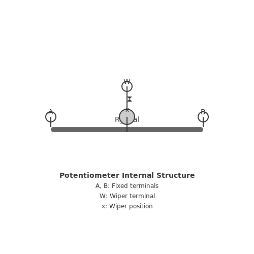
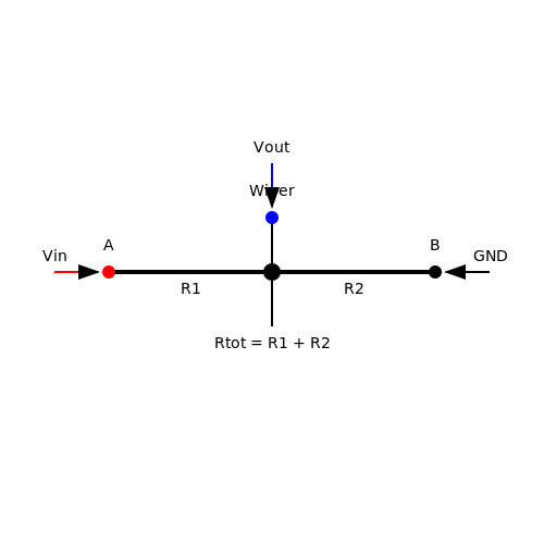
A potentiometer is a three-terminal resistive component used to provide an adjustable voltage division by mechanically varying the position of a sliding contact along a resistive element. Its operation is rooted in the fundamental principle of the voltage divider, where the output voltage Vout is a fraction of the input voltage Vin, determined by the ratio of resistances between the wiper and the terminals.
Mathematical Derivation
Consider a potentiometer with total resistance Rtot and a wiper that divides this resistance into two segments: R1 (between terminal A and the wiper) and R2 (between the wiper and terminal B). The output voltage Vout is derived from the voltage divider principle:
Since Rtot = R1 + R2, the equation simplifies to:
This linear relationship holds true for an ideal potentiometer with a uniform resistive track. However, real-world potentiometers may exhibit non-linearities due to material imperfections or manufacturing tolerances.
Construction and Types
Potentiometers are constructed using resistive materials such as carbon film, cermet, or conductive plastic. The resistive element can be linear (uniform resistance per unit length) or logarithmic (tapered resistance for audio applications). The mechanical interface—whether rotary or linear—determines the physical form factor and application suitability.
- Rotary potentiometers: Common in volume controls and angular position sensing.
- Linear potentiometers: Used in displacement measurement and fader controls.
- Digital potentiometers: IC-based variants with electronically controlled resistance values.
Practical Considerations
The resolution of a potentiometer is determined by the granularity of the wiper movement, while the power rating depends on the resistive material's ability to dissipate heat. Load effects must also be considered; connecting a low-impedance load to the wiper can introduce errors due to current draw, altering the expected voltage division.
In precision applications, multi-turn potentiometers or trimpots are employed to achieve finer adjustments. Environmental factors such as temperature and humidity can affect the resistive element's performance, necessitating derating or material-specific selection.
1.2 Construction and Internal Components
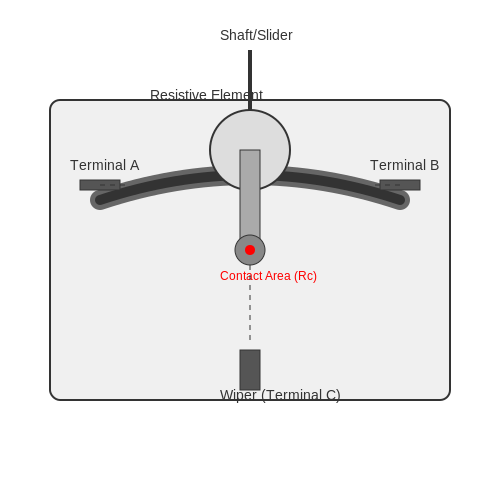
A potentiometer consists of three primary components: a resistive element, a sliding contact (wiper), and terminals. The resistive element is typically made from materials such as carbon composition, cermet, conductive plastic, or wirewound alloys, each offering distinct electrical and mechanical properties.
Resistive Element Materials
The choice of resistive material determines the potentiometer's performance characteristics, including resolution, noise, and power handling:
- Carbon Composition: A mixture of carbon particles and binder, offering moderate noise and reasonable lifespan. Commonly used in low-cost applications.
- Cermet: A ceramic-metal composite providing high stability and low temperature coefficient, ideal for precision applications.
- Conductive Plastic: Offers smooth operation and low noise, often used in high-resolution applications like audio equipment.
- Wirewound: Uses a resistive wire (e.g., nichrome) wound around a core, providing high power handling but limited resolution due to discrete winding steps.
Wiper Mechanism
The wiper is a movable contact that slides along the resistive track, typically made from a conductive alloy or precious metal to minimize contact resistance and wear. The mechanical interface between the wiper and resistive element introduces a contact resistance Rc, which can be modeled as:
where ρ is the resistivity of the contact material, A is the effective contact area, and FN is the normal force exerted by the wiper.
Terminal Configuration
Most potentiometers have three terminals: two fixed ends connected to the resistive element and a third connected to the wiper. In precision applications, a fourth terminal may be added to form a Kelvin connection, eliminating lead resistance errors.
Mechanical Construction
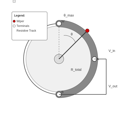
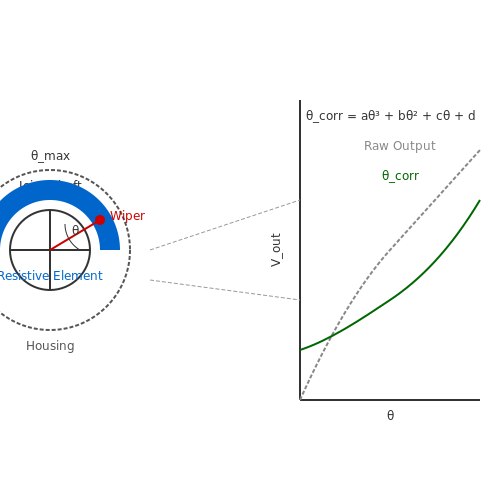
The resistive element is mounted on a substrate (often phenolic or ceramic) and enclosed in a housing that protects against environmental factors. Rotary potentiometers include a shaft and bearing assembly, while linear types use a slider mechanism. The mechanical angle θ of a rotary potentiometer relates to the output voltage Vout as:
where θmax is the maximum rotational angle (typically 270° to 300°).
1.3 Types of Potentiometers Based on Material
The resistive element of a potentiometer is a critical determinant of its performance, durability, and application suitability. The choice of material affects parameters such as temperature coefficient, noise, wear resistance, and power handling. Three primary materials dominate potentiometer construction: carbon composition, cermet, and wirewound, each with distinct advantages and limitations.
Carbon Composition Potentiometers
Carbon composition potentiometers employ a resistive track made from a mixture of carbon particles and a binder, typically phenolic resin. The resistivity ρ of the track is governed by the volumetric ratio of carbon to binder:
where ρ0 is the baseline resistivity at reference temperature T0, and α is the temperature coefficient (typically −200 to −500 ppm/°C). These potentiometers exhibit moderate noise levels (≈10–50 µV/V) due to granularity effects in the carbon matrix. Their primary advantage is low cost, but they suffer from limited resolution (≈5–10% of full scale) and wear-induced resistance drift after ≈50,000 cycles.
Cermet Potentiometers
Cermet (ceramic-metal) tracks consist of metal alloy particles (typically RuO2 or AgPd) sintered in a glass or ceramic matrix. The conduction mechanism follows percolation theory, with resistivity given by:
where ρm is the metal resistivity, ϕ is the volume fraction of metal, and t is the critical exponent (≈1.5–2.0). Cermet potentiometers offer superior temperature stability (α ≈ ±50 ppm/°C), low noise (<5 µV/V), and extended lifespan (>100,000 cycles). Their power rating reaches 2 W at 70°C, making them suitable for precision instrumentation and automotive applications.
Wirewound Potentiometers
Wirewound variants use a resistive wire (usually Nichrome or Karma alloy) wound around an insulating core. The resistance per unit length is:
where ρw is the wire resistivity and d is the diameter. These exhibit minimal noise (<1 µV/V) and handle high power (up to 100 W), but suffer from limited resolution due to discrete winding steps. The inductance L of the winding may become significant at frequencies above:
where R is the total resistance. Wirewound potentiometers are preferred in high-current applications like motor speed controls and industrial power systems.
Emerging Materials
Conductive polymer potentiometers (e.g., polyimide-carbon composites) provide ultra-smooth tracking with resolution <0.1% and cycle life exceeding 1 million operations. Their resistance follows a tunneling conduction model:
where d is inter-particle spacing, h is Planck's constant, m is electron mass, and ϕ is the barrier potential. These are increasingly used in medical devices and aerospace controls where micro-vibration resistance is critical.
2. Linear Potentiometers
2.1 Linear Potentiometers
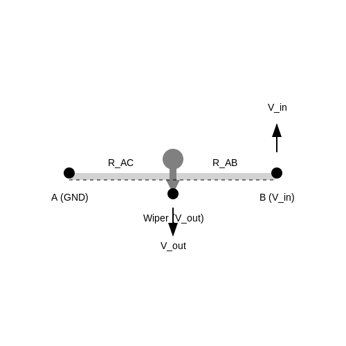
Linear potentiometers are three-terminal resistive devices where the output voltage varies linearly with the position of a sliding contact along a resistive element. The resistive track is typically made of conductive plastic, cermet, or wirewound materials, each offering distinct trade-offs in resolution, durability, and temperature stability. The voltage division principle governs their operation:
where RAC is the resistance between the wiper (terminal C) and ground (terminal A), and RAB is the total resistance across terminals A and B. For an ideal linear potentiometer, the output voltage scales proportionally with displacement x:
where L is the total travel length of the wiper. Non-linearity arises from imperfections in the resistive element, wiper contact resistance, or mechanical misalignment, often quantified as a percentage deviation from the ideal linear response.
Construction and Materials
Wirewound potentiometers use a helical resistive wire, offering high power handling (up to 100W) but limited resolution due to discrete turns. Conductive plastic variants provide near-infinite resolution (<0.1% nonlinearity) but lower maximum current (typically <1A). Cermet (ceramic-metal composite) tracks balance temperature stability (±100 ppm/°C) with moderate wear resistance.
Error Sources and Compensation
Load-induced nonlinearity occurs when an external load RL draws current from the wiper. The output voltage becomes:
For RL ≫ RAB, this effect diminishes. Temperature gradients along the resistive element introduce additional nonlinearity, particularly in wirewound designs where the temperature coefficient of resistance (TCR) can reach ±50 ppm/°C. Differential measurements or ratiometric configurations mitigate these errors.
Applications in Precision Systems
High-precision linear potentiometers (e.g., Beckman Helipot series) achieve ±0.05% linearity in aerospace and medical equipment. In servo feedback systems, their low phase lag (<1μs) makes them preferable to optical encoders for real-time position control. Multi-turn variants with spiral tracks extend measurement range while maintaining sub-millimeter resolution.
2.2 Rotary Potentiometers
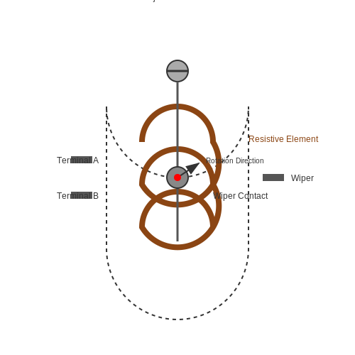
Rotary potentiometers are electromechanical devices that convert angular displacement into a variable resistance. Their operation relies on a resistive element, typically a carbon or conductive plastic track, and a sliding contact (wiper) that moves along the track as the shaft rotates. The resistance between the wiper and either end terminal varies linearly or logarithmically with the rotation angle.
Construction and Working Principle
A rotary potentiometer consists of three terminals: two fixed end terminals (A and B) connected to the resistive track and a third terminal (W) attached to the wiper. The total resistance Rtotal between terminals A and B remains constant, while the resistance between the wiper and either terminal varies with shaft position. For a linear taper potentiometer, the output voltage Vout follows:
where θ is the rotation angle and θmax is the maximum rotational range (typically 270° to 300°). Logarithmic taper potentiometers follow an exponential relationship, making them suitable for audio applications where human hearing responds logarithmically to sound intensity.
Mathematical Derivation of Linearity
Assuming a uniform resistive track with resistivity ρ and cross-sectional area A, the resistance per unit angle is constant. For a rotation angle θ, the resistance R1 between terminal A and the wiper is:
The output voltage divider relationship is then:
Types of Rotary Potentiometers
- Single-Turn: Limited to one full rotation (≈300°), commonly used for volume controls and basic voltage division.
- Multi-Turn: Allows multiple rotations (e.g., 5, 10, or 25 turns) for precise adjustments, often found in calibration equipment.
- Servo Mount: Designed for integration with servo motors, featuring a splined shaft for direct coupling.
Nonlinear Tapers
For logarithmic (audio) taper potentiometers, the resistance follows:
where k is a scaling factor. This ensures a logarithmic response to match perceptual loudness curves in audio applications.
Practical Considerations
Key performance parameters include:
- Resolution: Determined by the wiper contact's finite width, limiting the smallest detectable angle change.
- Power Rating: Typically 0.1W to 2W, constrained by resistive track material and heat dissipation.
- Mechanical Life: Carbon track potentiometers endure 10,000–50,000 cycles, while conductive plastic variants exceed 100,000 cycles.
Applications
Rotary potentiometers are ubiquitous in:
- Audio equipment (volume, tone controls)
- Industrial control systems (position feedback, calibration)
- User interface devices (knobs, dials)
2.3 Digital Potentiometers
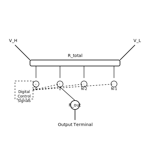
Digital potentiometers (digipots) are solid-state devices that emulate the functionality of mechanical potentiometers but are controlled digitally via serial interfaces such as I²C, SPI, or simple up/down signals. Unlike their analog counterparts, they offer precise, repeatable adjustments without mechanical wear, making them ideal for applications requiring automated calibration, programmable gain amplifiers, or digital volume control.
Architecture and Operation
A digital potentiometer consists of a resistor ladder network with electronically controlled switches (typically MOSFETs or CMOS transmission gates) that select tap points. The resolution of a digipot is determined by the number of steps in the ladder, commonly ranging from 32 to 256 steps (5 to 8 bits). The equivalent resistance between the wiper (W) and terminal ends (A, B) is given by:
where RAB is the end-to-end resistance, D is the digital input code, and n is the resolution in bits. For example, an 8-bit digipot with RAB = 10 kΩ at code D = 128 yields:
Non-Ideal Characteristics
Key non-idealities include:
- Wiper resistance (RW): Typically 50–500 Ω, adding a parasitic series resistance.
- Temperature coefficient: Often ±300 ppm/°C, affecting stability in precision circuits.
- Voltage limitations: CMOS-based digipots often restrict terminal voltages to supply rails.
- Bandwidth: Limited by stray capacitance (10–100 pF) and switch impedance.
Applications and Trade-offs
Digital potentiometers are widely used in:
- Programmable gain amplifiers (PGAs) for sensor signal conditioning.
- LCD contrast or backlight adjustment in embedded systems.
- Automated test equipment for dynamic load simulation.
However, they are unsuitable for high-power applications (due to current limitations) or ultra-high-precision circuits (due to wiper resistance and thermal drift). Hybrid solutions, such as digitally controlled rheostats with external power FETs, may bridge this gap.
Interface and Control
Modern digipots integrate non-volatile memory (EEPROM or flash) to retain settings during power cycles. For example, the AD5245 (I²C interface) allows daisy-chaining and supports 256-tap resolution. Below is a simplified SPI interface timing diagram for a typical digipot:
2.4 Trimmer Potentiometers
Trimmer potentiometers, also known as trimpots, are miniature adjustable resistors designed for infrequent calibration or tuning in electronic circuits. Unlike standard potentiometers, they are optimized for precision adjustments during circuit assembly or maintenance rather than continuous user interaction.
Construction and Operating Principle
Trimpots employ either cermet (ceramic-metal composite) or conductive plastic resistive tracks, with a mechanical wiper contact moved by a screwdriver-adjustable shaft. The resistance follows the standard potentiometer relationship:
where θ represents the rotation angle and θmax the mechanical travel limit. High-precision variants achieve ±10% tolerance or better through laser trimming during manufacturing.
Key Performance Parameters
- Resolution: Typically 0.25% to 1% of full scale for single-turn models
- Temperature Coefficient: 100-300 ppm/°C for cermet, 50-150 ppm/°C for conductive plastic
- Rotational Life: 100-200 cycles (vs. 50,000+ for panel pots)
- Power Rating: Usually 0.1W to 0.5W at 70°C
Circuit Applications
Trimpots serve critical functions in analog circuit calibration:
where R2 represents the adjustable trimpot resistance. Common implementations include:
- Bias current adjustment in op-amp circuits
- LCD contrast voltage tuning
- Oscillator frequency trimming (e.g., in crystal clock circuits)
- Sensor calibration offsets
Mounting and Environmental Considerations
Surface-mount (SMD) trimpots dominate modern designs, with through-hole versions persisting in high-vibration environments. Conformal coating compatibility varies by model - silicone-based coatings are preferred for their non-wicking properties. The adjustment screw typically requires 1.5-3.5mm flathead or Phillips drivers, with some models incorporating slotted or knurled knobs for tool-less adjustment.
Advanced Variants
Multi-turn trimpots (3-25 turns) provide enhanced resolution through gear reduction mechanisms. Digital trimpots (digipots) offer programmable resistance via I²C or SPI interfaces, though with higher temperature drift (500-1000 ppm/°C). Hermetically sealed versions maintain stable resistance in humid or corrosive environments.
3. Voltage Division Principle
3.1 Voltage Division Principle
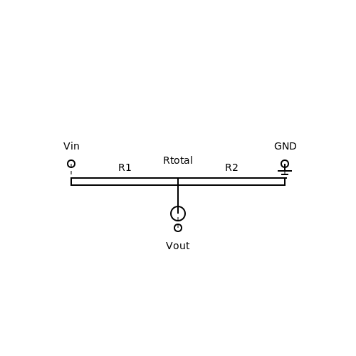
The voltage division principle is fundamental to understanding how potentiometers function as adjustable voltage dividers. At its core, a potentiometer consists of a resistive element with three terminals: two fixed end terminals and a movable wiper. When a voltage is applied across the end terminals, the wiper position determines the output voltage, which is a fraction of the input voltage.
Mathematical Derivation
Consider a potentiometer with total resistance Rtotal and wiper positioned such that the resistance between the wiper and one terminal is R1, and between the wiper and the other terminal is R2. The output voltage Vout is derived as follows:
Since Rtotal = R1 + R2, the equation simplifies to:
This linear relationship holds true for ideal potentiometers, where the resistive element is uniform and the wiper contact resistance is negligible.
Practical Considerations
In real-world applications, several factors influence the accuracy of voltage division:
- Resistive Taper: The resistive element may have a linear or logarithmic taper, affecting the voltage division proportionality.
- Wiper Contact Resistance: Non-ideal contacts introduce additional resistance, leading to deviations from the ideal output.
- Load Effects: Connecting a load to the wiper terminal draws current, altering the effective voltage division ratio.
Applications in Circuit Design
The voltage division principle is widely applied in:
- Signal Conditioning: Adjusting sensor output levels to match ADC input ranges.
- Biasing Circuits: Setting reference voltages in amplifier stages.
- User Interfaces: Volume controls and brightness adjustments in consumer electronics.
Non-Ideal Behavior and Compensation
For precision applications, compensating for non-ideal effects is critical. Techniques include:
- Using buffer amplifiers to isolate the wiper from load effects.
- Selecting potentiometers with low wiper contact resistance.
- Employing multi-turn potentiometers for fine adjustment resolution.
The voltage division principle extends beyond potentiometers to resistor networks and integrated voltage dividers, forming the basis for many analog circuit designs.
3.2 Taper and Resistance Curve
The taper of a potentiometer defines how the output voltage or resistance varies as a function of the wiper position. Unlike a linear potentiometer, where resistance changes uniformly with rotation, tapered potentiometers exhibit nonlinear behavior, making them critical in applications requiring logarithmic or other non-uniform responses.
Mathematical Representation of Taper
The resistance curve R(θ) of a potentiometer as a function of rotation angle θ can be expressed as:
where Rtotal is the total resistance and f(θ) is the taper function, which determines the resistance distribution. For a linear potentiometer, f(θ) = θ/θmax, but nonlinear tapers introduce more complex functions.
Common Taper Types
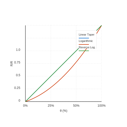
Three primary taper types dominate practical applications:
- Linear Taper: Resistance changes proportionally with wiper position. The transfer function is f(θ) = kθ, where k is a constant.
- Logarithmic (Audio) Taper: Resistance follows a logarithmic curve, making it ideal for volume controls due to human hearing's logarithmic sensitivity. The function approximates f(θ) = log(θ/θmax + 1).
- Reverse Logarithmic Taper: Similar to logarithmic but inverted, often used in specialized audio and lighting controls.
Derivation of Logarithmic Taper
A logarithmic taper potentiometer is designed to match the human ear's perception of sound intensity, which follows a power-law relationship. The resistance curve can be modeled as:
where k is a scaling factor. For practical implementations, manufacturers often approximate this using segmented resistive elements or composite materials.
Practical Applications
- Audio Equipment: Logarithmic potentiometers are standard in volume and tone controls to ensure perceived linearity in sound adjustment.
- Industrial Controls: Custom tapers are used in process automation where sensor responses require nonlinear scaling.
- Light Dimmers: Reverse logarithmic tapers help match human brightness perception.
Manufacturing Techniques
Nonlinear tapers are achieved through:
- Segmented Resistive Tracks: Discrete resistive sections with varying compositions.
- Conductive Plastic Blending: Adjusting material resistivity along the track.
- Hybrid Designs: Combining carbon and cermet elements for precise nonlinearity.
The above diagram illustrates the resistance curves for different tapers, with the x-axis representing wiper position (θ) and the y-axis representing normalized resistance (R/Rtotal).
Power Rating and Tolerance
Power Dissipation and Thermal Limits
The power rating of a potentiometer defines the maximum power it can dissipate without sustaining damage. For resistive elements, power dissipation follows Joule's law:
where P is power in watts, I is current in amperes, and R is resistance in ohms. However, this equation assumes ideal conditions. In practice, derating is necessary due to thermal effects. The power rating decreases with ambient temperature, often specified in derating curves by manufacturers. For example, a 1W potentiometer may only handle 0.5W at 70°C.
Tolerance and Resistance Accuracy
Tolerance indicates the permissible deviation from the nominal resistance value, expressed as a percentage. A 10kΩ potentiometer with ±10% tolerance may measure between 9kΩ and 11kΩ. For precision applications, wirewound or conductive plastic potentiometers offer tolerances as tight as ±1%. The tolerance affects:
- Voltage division accuracy in rheostat configurations.
- Linearity in position-sensitive circuits.
- Stability under thermal or mechanical stress.
Derating and Real-World Considerations
Power ratings assume free airflow and ideal heat dissipation. In enclosed spaces or high-density PCB layouts, thermal resistance (RθJA) becomes critical. The maximum allowable power must satisfy:
where Tjmax is the maximum junction temperature (e.g., 125°C for carbon composition) and Tambient is the operating environment temperature. Forced cooling or heatsinking may be required in high-power applications.
Case Study: Audio Taper Potentiometers
In audio applications, logarithmic-taper potentiometers must maintain tight tolerance across their rotation to preserve signal integrity. A 20% tolerance in resistance could introduce audible distortion or channel imbalance. High-end models use laser-trimmed resistive tracks to achieve ±3% tolerance while dissipating up to 0.5W continuously.
Material Impact on Power Handling
Wirewound potentiometers excel in high-power scenarios (up to 100W) due to their low temperature coefficient of resistance (TCR) and robust construction. In contrast, cermet or conductive plastic variants, while precise, typically max out at 2W due to material limitations. The trade-off between precision and power handling is a key design consideration.
4. Volume Control in Audio Devices
Volume Control in Audio Devices
Fundamentals of Audio Attenuation
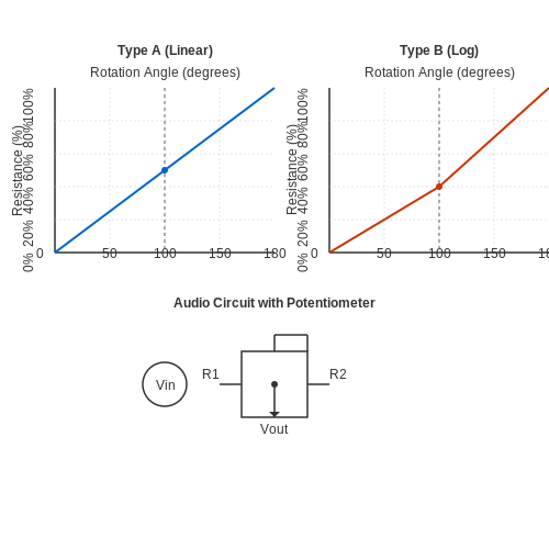
In audio circuits, a potentiometer functions as a voltage divider, attenuating the signal amplitude before it reaches the amplifier stage. The resistive track's wiper position determines the output voltage fraction, governed by:
Where R1 is the resistance between the input and wiper, and R2 is the resistance between the wiper and ground. Logarithmic taper potentiometers (Type B) are preferred over linear taper (Type A) for volume control due to the human ear's logarithmic response to sound pressure levels (Weber-Fechner law).
Logarithmic vs. Linear Taper
The perceived loudness L follows a power-law relationship with signal voltage:
A logarithmic potentiometer compensates for this by providing finer control at lower volumes. The resistance curve approximates:
where θ is the rotation angle (0-1) and k is a constant determining the curve steepness.
Circuit Implementation
Modern audio systems often use dual-gang potentiometers for stereo channels, with matched resistances (±20%) to maintain channel balance. The equivalent circuit includes:
- Source impedance (typically 50Ω-600Ω)
- Potentiometer value (10kΩ-100kΩ for line-level signals)
- Amplifier input impedance (>50kΩ to prevent loading)
Advanced Considerations
Noise Performance
Carbon composition potentiometers exhibit 1/f noise due to granular resistance material. Conductive plastic potentiometers (50,000+ cycles lifespan) offer lower noise (≤-120dB) at the cost of higher price. The noise voltage spectral density follows:
Digital Alternatives
Digital potentiometers (e.g., DS1802) provide microcontroller-controlled attenuation with 256+ steps. However, they introduce quantization distortion and typically have higher THD (0.01% vs. 0.001% for analog pots) due to MOSFET switch resistance nonlinearities.
Practical Design Guidelines
- Use 20% derating for power dissipation (Pmax ≤ 0.8·(V2/Rtotal))
- Maintain signal-to-ground impedance ratio >10:1 to prevent high-frequency roll-off
- For phono preamps, select pots with <5pF parasitic capacitance to preserve RIAA equalization
Position Sensing in Robotics
Potentiometers serve as highly effective position sensors in robotic systems due to their simplicity, reliability, and analog output proportional to angular or linear displacement. In robotic joints, a rotary potentiometer is often coupled directly to the actuator shaft, providing real-time feedback on joint angle. The voltage divider principle governs their operation:
where Vout is the output voltage, Vin is the supply voltage, Rwiper is the resistance between the wiper and ground, and Rtotal is the potentiometer's total resistance. This linear relationship enables precise position tracking when calibrated.
Robotic Joint Angle Measurement
For a robotic arm with n degrees of freedom, each joint requires independent angle measurement. A multi-turn potentiometer can be employed for applications requiring rotation beyond 360°. The resolution Δθ of the measurement depends on the potentiometer's resistive element linearity and the analog-to-digital converter (ADC) bit depth:
where θmax is the maximum rotational range and N is the ADC bit resolution. For a 10-bit ADC and 300° range, Δθ ≈ 0.29°, sufficient for many industrial robots.
Nonlinearity Compensation
Despite their inherent linearity, potentiometers exhibit deviations due to manufacturing tolerances and wear. A calibration curve can be derived using a high-precision encoder as reference. The corrected angle θcorr is computed via polynomial fitting:
where coefficients a0...n are determined through least-squares regression. This compensates for both integral nonlinearity (INL) and differential nonlinearity (DNL).
Practical Implementation Considerations
- Mechanical Loading: The potentiometer's torque requirement must not exceed the actuator's backdrive capability.
- Signal Conditioning: Low-pass filtering (cutoff frequency fc ≤ 0.1 fsampling) mitigates noise from PWM-driven motors.
- Wear Mitigation: Conductive plastic potentiometers offer >10 million cycles lifespan, compared to <1 million for carbon film types.
Case Study: SCARA Robot Wrist Joint
A 4-axis SCARA robot employs 10kΩ conductive plastic potentiometers with 0.25% linearity tolerance for wrist positioning. The voltage output is digitized by a 12-bit ADC (LSB = 0.024% of full scale), yielding ±0.036° repeatability. The system achieves ±0.1° absolute accuracy after third-order polynomial correction.
4.3 Calibration and Tuning in Circuits
Precision calibration of potentiometers is critical in applications requiring fine-tuned voltage division or resistance matching. Unlike basic trimming, advanced calibration involves compensating for nonlinearities, temperature drift, and mechanical wear while maintaining stability under dynamic load conditions.
Mathematical Basis for Calibration
The transfer function of an ideal linear potentiometer is given by:
However, real potentiometers exhibit deviations due to resistive track imperfections. The actual wiper position θ (mechanical rotation angle) relates to resistance via a nonlinear correction term f(θ):
where kn represents harmonic distortion coefficients measurable through Fourier analysis of resistance sweeps.
Closed-Loop Calibration Techniques
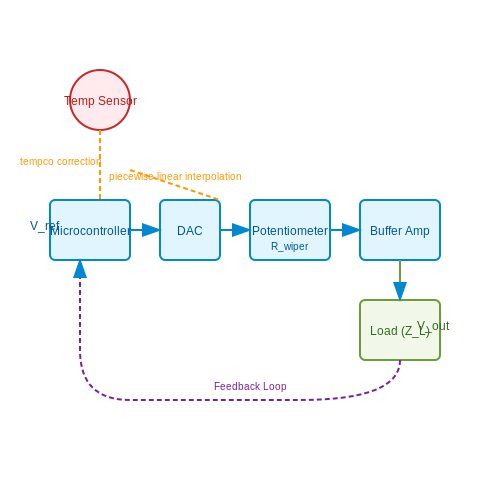
For precision instrumentation, a feedback-based approach using a microcontroller and DAC achieves sub-millivolt accuracy:
- Apply known reference voltages Vref across the potentiometer
- Measure actual output Vout at multiple wiper positions
- Construct a lookup table (LUT) mapping commanded vs. actual positions
- Implement piecewise linear interpolation between calibration points
Temperature compensation requires characterizing the tempco of the resistive element (typically 100-300 ppm/°C for cermet or conductive plastic) and implementing either:
- Analog compensation: Paired with NTC/PTC thermistors in the feedback path
- Digital compensation: Polynomial correction based on onboard temperature sensor data
Dynamic Load Considerations
Loading effects become significant when downstream impedance ZL approaches the potentiometer's output impedance. The modified voltage divider equation accounts for this:
For high-precision applications, buffer amplifiers with input impedance >1012 Ω eliminate loading errors while maintaining calibration integrity.
Case Study: Synchro-Resolvers in Aerospace
Military-grade synchro-resolvers use multi-turn wirewound potentiometers with laser-trimmed compensation networks. Calibration involves:
- Mechanical backlash measurement using hysteresis loops
- Contact resistance testing at 10 mA wetting current
- Vibration testing to validate wiper stability under 15g RMS
The resulting calibration curves achieve ±0.01% linearity across -55°C to +125°C operational ranges.
Automated Calibration Systems
Modern production lines employ computer-controlled calibration rigs featuring:
- 6-axis robotic wiper actuators with 0.001° angular resolution
- Four-wire Kelvin resistance measurement
- Statistical process control (SPC) for tracking long-term drift
These systems perform 100% testing on precision potentiometers, storing calibration coefficients in onboard EEPROM for field-replaceable units.
5. Choosing the Right Potentiometer
5.1 Choosing the Right Potentiometer
Selecting an appropriate potentiometer requires a thorough understanding of electrical parameters, mechanical constraints, and environmental factors. The primary considerations include resistance value, tolerance, power rating, taper, and construction type, each of which influences performance in specific applications.
Resistance Value and Tolerance
The nominal resistance value, typically measured in ohms (Ω), determines the potentiometer's range of adjustment. For precision applications, tolerance—expressed as a percentage deviation from the nominal value—becomes critical. High-precision potentiometers exhibit tolerances as low as ±1%, while general-purpose variants may range from ±5% to ±20%.
Power Rating and Derating
The power rating specifies the maximum wattage the potentiometer can dissipate without damage, calculated as:
However, derating is necessary at elevated temperatures. For example, a 1W-rated potentiometer may only handle 0.5W at 70°C. Always consult the manufacturer’s derating curve for thermal performance.
Taper Characteristics
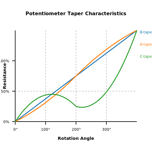
The taper defines the relationship between the wiper position and resistance. Common tapers include:
- Linear taper (B-taper): Resistance changes uniformly with rotation.
- Logarithmic taper (A-taper): Resistance follows a logarithmic curve, ideal for audio volume controls.
- Anti-logarithmic taper (C-taper): Inverse of logarithmic, used in specialized applications.
Mechanical and Environmental Considerations
Operational lifespan is determined by mechanical endurance, typically rated in cycles (e.g., 50,000 rotations). Environmental factors include:
- IP Rating: Ingress protection against dust and moisture.
- Temperature Range: Industrial-grade potentiometers operate from -40°C to 125°C.
- Vibration Resistance: Critical for automotive or aerospace applications.
Construction Types
Different constructions suit varying use cases:
- Wirewound: High power handling but limited resolution due to discrete winding steps.
- Cermet: Ceramic-metal composite offering stability and precision.
- Conductive Plastic: Smooth adjustment and high resolution, ideal for sensitive controls.
Noise and Contact Resistance
In high-impedance circuits, contact resistance variations introduce noise. Gold-plated contacts minimize this effect, while lubricants reduce wear-induced fluctuations.
Application-Specific Selection
For audio equipment, logarithmic potentiometers with low noise are preferred. In power electronics, wirewound types with high wattage ratings dominate. Precision instrumentation demands cermet or conductive plastic potentiometers with tight tolerances.
5.2 Wiring and Connection Methods
Basic Three-Terminal Configuration
The standard potentiometer consists of three terminals: the input (or fixed) terminal (A), the output (or wiper) terminal (W), and the ground (or reference) terminal (B). The resistive element between A and B forms a voltage divider, with the wiper W providing a variable output voltage proportional to its position. The voltage division ratio is given by:
where RWB is the resistance between the wiper and terminal B, and RAB is the total resistance between terminals A and B. For linear taper potentiometers, the output voltage varies linearly with the wiper position, while logarithmic taper potentiometers exhibit an exponential response.
Voltage Divider Implementation
When used as a voltage divider, the potentiometer is connected between a voltage source (Vin) and ground. The wiper terminal provides the adjustable output voltage. The current through the potentiometer is:
To minimize power dissipation, the potentiometer's resistance should be chosen such that I does not exceed its power rating. For precision applications, low-temperature-coefficient (low-TC) resistors should be used to minimize drift.
Rheostat Mode (Two-Terminal Configuration)
In rheostat mode, the potentiometer acts as a variable resistor by connecting only the wiper (W) and one fixed terminal (A or B). This configuration is useful for current control applications, such as adjusting LED brightness or motor speed. The equivalent resistance is:
Care must be taken to avoid open-circuit conditions, which can damage the wiper contact due to excessive current.
Digital Potentiometers
Digital potentiometers (digipots) replace the mechanical wiper with electronically controlled switches, enabling programmable resistance adjustment. They are interfaced via I²C, SPI, or other digital protocols. The resolution of a digipot is given by:
where N is the number of bits. For example, a 10-bit digipot with RAB = 10 kΩ has a resolution of ≈9.77 Ω per step.
Noise and Stability Considerations
Mechanical potentiometers are susceptible to contact noise, which manifests as erratic output fluctuations. To mitigate this, conductive plastic or cermet elements are preferred over carbon composition. For high-frequency applications, parasitic capacitance (Cp) and inductance (Lp) must be considered, as they form an unintended RLC network with the potentiometer's resistance.
Practical Applications
- Audio Equipment: Logarithmic potentiometers are used for volume control due to their perceptual response matching human hearing.
- Sensor Calibration: Precision multiturn potentiometers provide fine adjustments in bridge circuits and transducer interfaces.
- Feedback Systems: Potentiometers serve as position sensors in servo mechanisms, where their analog output is proportional to angular or linear displacement.
SPICE Simulation Example
To model a potentiometer in SPICE, a subcircuit with a variable resistor can be implemented. The following netlist snippet demonstrates a 10 kΩ linear potentiometer with the wiper at 50% position:
* Potentiometer SPICE Model
V1 1 0 DC 5
R1 1 2 5k
R2 2 0 5k
.tran 1m 1
.end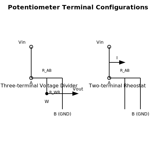
5.3 Common Pitfalls and Troubleshooting
Electrical Noise and Contact Resistance
Potentiometers are susceptible to electrical noise due to mechanical wear and oxidation of the resistive track. The contact resistance between the wiper and the track can introduce nonlinearities and signal degradation. For high-precision applications, the noise voltage Vn can be modeled as:
where kB is Boltzmann's constant, T is temperature, R is resistance, and Δf is the bandwidth. To mitigate this, use conductive plastic or cermet potentiometers with lower noise characteristics.
Mechanical Wear and Lifespan
Mechanical wear is a dominant failure mode in potentiometers, particularly in high-cycle applications. The lifespan L (in cycles) can be approximated by:
where Fmax is the maximum allowable force, Fapplied is the operational force, and n is a material-dependent exponent (typically 2–3). Lubrication and reduced wiper pressure can extend lifespan.
Temperature Coefficient and Drift
Temperature variations cause resistance drift, quantified by the temperature coefficient of resistance (TCR):
Carbon composition potentiometers exhibit TCR values of ±500 ppm/°C, while precision wirewound types achieve ±10 ppm/°C. For stable operation, select materials with low TCR or implement temperature compensation.
Load Effects and Nonlinearity
Loading effects occur when the potentiometer's output is connected to a low-impedance load, distorting the voltage divider relationship. The actual output voltage Vout deviates from the ideal:
where RL is the load resistance. To minimize error, ensure RL ≫ Rpot or buffer the output with an op-amp.
Intermittent Connections
Intermittent wiper contact causes signal dropouts, often due to dust, oxidation, or mechanical misalignment. A first-order model for contact reliability Pc is:
where λ is the failure rate. Sealed or hermetically enclosed potentiometers reduce contamination risks.
Common Troubleshooting Steps
- Noisy Output: Check for oxidation, clean the track with contact cleaner, or replace with a low-noise type.
- Dead Spots: Measure resistance across the track to identify worn regions. Replace if uneven wear exceeds 10%.
- Drifting Values: Verify TCR compatibility with operating conditions. Use a stable voltage reference for calibration.
- Mechanical Play: Inspect wiper alignment and spring tension. Excessive play indicates wear or manufacturing defects.
6. Recommended Books and Articles
6.1 Recommended Books and Articles
- PDF IEEE Std C57-113-1991 (Revision and redesignation of IEEE Std C57-113 ... — in the form of a calibrated potentiometer or a calibrated step attenuator should be provided. The adjustment range should extend over at least two decades, and a minimum of three adjusting steps, per decade should be provided. A calibrated adjustment is not required if the generator output level is monitored. Adjusting its output level should not
- 3.6: Potentiometer as a Voltage Divider - Workforce LibreTexts — Book: Electric Circuits VI - Experiments (Kuphaldt) ... Potentiometer, multi turn, 1 kΩ to 20 kΩ, (Radio Shack catalog # 271-342, 271-343, 900-8583, or 900-8587 through 900-8590) ... Recommended articles. Article type Section or Page Author Tony R. Kuphaldt License GNU FDL License Version 1.3;
- PDF ELECTRICAL MEASUREMENTS & INSTRUMENTATION - Veer Surendra Sai ... — assignments by referring the text books and reference books. Further, this document is not ... Potentiometers: DC Potentiometer, Crompton potentiometer, construction, standardization, application. ... Draw the block diagram of an electronic voltmeter and explain its operation. [5] 8. Write short notes on: [5X2] ...
- Potentiometric Titration - an overview | ScienceDirect Topics — Potentiometric titration is considered to be the most consistent and robust technique among the non-NMR methods (Czechowska-Biskup, 2012).However, some of the disadvantages include the time-consuming and labor-intensive nature of measurements and the requirement of solutions of accurately known concentrations (Dimzon and Knepper, 2015).In potentiometric titration, a known quantity of chitosan ...
- L-pad, potentiometer, volume control - Whats the difference? - AudioReview — Use a standard Potentiometer if you want a knob to adjust settings. You will probably also want "Audio Taper" pots, and not "Linear Taper" for this application. The nature of your question warrants a proper answer and honestly it would be bit wordy for this media - maybe read up on a few "How to" electronics books would help.
- PDF First Edition, last update November 06, 2021 - The Public's Library and ... — hands-on experimentation. Knowledge gleaned from books alone has limited use, especially in scientific endeavors. If my contribution to society is to be complete, I must include a guide to experimentation along with the text(s) on theory, so that the individual learning on their own has a resource to guide their experimental adventures.
- Potentiometers - an overview | ScienceDirect Topics — The potentiometric measurements are perhaps the most accomplished in the instrumental chemical analysis, being that of the hydrogenation potential is the best known and applied. The basic structure of a potentiometer is composed of reference electrode, indicating electrode (or work electrode) and a potential measuring device.
- Potentiometric Sensing | Analytical Chemistry - ACS Publications — For the best membrane composition, the logarithmic selectivity coefficients were about −3.5 over Pb 2+ and Cd 2+ and about −4.5 over Zn 2+ and Ni 2+. While the ionophores were considered to be neutral carriers, it is not clear why the incorporation of anionic lipophilic sites into the membrane composition deteriorated the ISE response.
- Transducers - SpringerLink — Potentiometer resistance, gauge, resistance strain gauge, resistance thermometer and thermistor are some of the examples of resistance transducers. 6.4.2 Potentiometer (POT) It is a passive device with a thin wire of platinum or nickel alloy of 0.01 mm diameter carefully wound on an insulated former.
- Potentiometry - an overview | ScienceDirect Topics — The apparatus was thermostatted within ±0.5K Constant values of the emf were measured by a potentiometer with a precision of ±0.1 mV. The results obtained are presented in Fig. 9.4 . The limits of the potential plateau define precisely the existence of the (Li) + (Mg) two-phase region.
6.2 Online Resources and Datasheets
- Potentiometers Datasheets - Mouser - Mouser Electronics — Potentiometers are available at Mouser Electronics. Mouser offers inventory, pricing, & datasheets for Potentiometers. ... & datasheets for Potentiometers. Skip to Main Content (800) 346-6873. Contact Mouser (USA) (800) 346-6873 | Feedback. Change Location. English. Español ... Resources. Blog; Newest Products; New Manufacturers; Applications ...
- ADALP2000 Product Description [Analog Devices Wiki] — Datasheet : SQP10AJB-6R2 : 6.2 Ω 10W Power Resistor Axial Cement Link: Datasheet * 3386C-1-502LF * 3386C-1-103LF * 3386C-1-503LF * Single Turn 5 kΩ Potentiometer * Single Turn 10 kΩ Potentiometer * Single Turn 50 kΩ Potentiometer : Datasheet: 2N3904 : NPN General Purpose Transistor TO-92 Link Marking: 2N3904 : Datasheet: 2N3906
- PDF Long Life Cermet Potentiometer 2 Million Cycles - Vishay Intertechnology — Long Life Cermet Potentiometer 2 Million Cycles LINKS TO ADDITIONAL RESOURCES FEATURES • 2 million cycles • Cermet element • 12.5 mm square single turn panel control • 4, 6 and 6.35 shaft diameters and 29 terminal styles • Multiple assemblies - up to four modules • Test according to CECC 41000 or IEC 60393-1 • Low temperature ...
- PDF TPL0202 256-Taps Dual Channel Digital Potentiometer With SPI and Non ... — potentiometers (DPOTs) with 256 wiper positions. Each potentiometer can be used as a three-terminal potentiometer or as a two-terminal rheostat. The TPL0202-10 has an end-to-end resistance of 10 kΩ. This DPOT can be used as a mechanical potentiometer replacement, allowing the user (or software) to digitally control and adjust resistance.
- PDF TPL0102 Two 256-Taps Digital Potentiometers With Non-Volatile Memory — • Mechanical Potentiometer Replacement 3 Description The TPL0102 has two linear-taper digital potentiometers (DPOTs) with 256 wiper positions. Each potentiometer can be used as a three-terminal potentiometer or as a two-terminal rheostat. The TPL0102-100 has an end-to-end resistance of 100 kΩ. The TPL0102 has non-volatile memory (EEPROM)
- PDF Knob Operating Type Potentiometer With Knob Type - RS Components — Potentiometers Rotary Potentiometers With Knob Type RK10J/RK14J Series Low-profile, dip and reflow solderable. ... 7.6 2 8 14 ø14 0.8 4 5.35 6 8.5 9.5 0.3 3.2 2.5 0.9 1 Center of knob Solder lands are indicated by the shaded areas ... DATASHEET, PDF DATASHEET, IC, CHIP, SEMICONDUCTOR, TRANSISTOR, ELECTRONIC COMPONENT, ISO COMPONENT ...
- ALLDATASHEET.COM - Electronic Parts Datasheet Search — ALLDATASHEET.COM is the biggest online electronic component datasheets search engine. - Contains over 50 million semiconductor datasheets. - More than 60,000 Datasheets update per month. - More than 460,000 Searches per day. - More than 28,000,000 Impressions per month.
- PDF Potentiometers and Trimmers - Vishay Intertechnology — A potentiometer with two or mo re sections, each electrically independent, operated by a common spindle. 1.4 - Multi-turn potentiometer A potentiometer with a shaft rotation of more than 360° from one end of the resistive element to the other. Multi-turn types are usually trimming or precision potentiometers. 1.5 - Sealed potentiometers
- PDF Carbon Potentiometers CA - ACP Technologies — Shafts can be sold separately or delivered already mounted on the potentiometer at ACP. When a shaft is mounted on a potentiometer, the distance from the top of the potentiometer to the top of the shaft is marked with "L" in the table below, as shown in the drawings: H potentiometer + shaft V potentiometer + shaft L Dimension Shaft 10 6022 ...
- PDF Digital Potentiometers Design Guide - Microchip Technology — SOT-23-5 package. The potentiometer pinout with all terminals available requires an 8-pin package. Dual potentiometer options allow the customer to have potentiometers/variable resistors that are closely matched in the system, since the two devices are on the same device die. Packaging options allow customers to address their
6.3 Advanced Topics and Research Papers
- Prithwiraj Purkait-Electrical and Electronics Measurements ... - 1Library — Dr Purkait has published extensively in international journals and conference proceedings on various topics related to his research paradigm. ... = 205.3 × 10⁻⁶ — 201.4 × 10-6 = 3.9 × 10⁻⁶ F = 3.9 × 10⁻⁶ F Example 1.7 ... International Journal of Advanced Research in Electrical, Electronics and Instrumentation Engineering 13. 0. 0.
- 6.3 - Analog Read and the Potentiometer | High School Maker — To wire up the potentiometer you connect the center lead to analog pin 2. The two sides get hooked to power. One side goes to positive volts and the other goes to the ground. If you look in the Black Case labeled "Regular Components" you should be able to find some Potentiometers that are easy to use with your breadboards.
- PDF Chapter 6 Potentiometric Sensors - Springer — 122 6 Potentiometric Sensors π0 = μ0,S i −μ 0,m i z iF (6.5) Thus, the Nernst equation relates the potential differenceπ= ϕβ−ϕs at the inter- face to the activities of species i in phases m and S.The standard state of the metal
- PDF Fundamentals of Measurements Potentiometers & Bridges — POTENTIOMETERS & BRIDGES 2.1 D.C. potentiometer, principle, working and list of applications. 2.2 Wheatstone bridge and Kelvin's double bridge for resistance measurement. ... A course in electronics & electrical measurement & instrumentation By J.B.Gupta - Ketson 5. Principles of measurement & Instumentation By A.S.Morris - PHI .
- Potentiometry Research Papers - Academia.edu — In this paper a comparison about kinetic behaviour, acid-base properties and copper removal capacities was carried out between two different adsorbent materials used for heavy metal removal from aqueous solutions: an aminodiacetic chelating resin as commercial product (Lewatit TP207) and a lyophilised bacterial biomass of Sphaerotilus natans.
- PDF Advanced Potentiometry - Springer — any means, electronic, mechanical, photocopying, microfilming, recording or otherwise, without written permission from the Publisher, with the exception of any material supplied specifically for the purpose of being entered and executed on a computer system, for exclusive use by the purchaser of the work. Printed on acid-free paper
- Electronic potentiometer cell using a CMOS floating-gate memory — This paper describes the experimental design of an electronic potentiometer cell (e-pot) to provide reference voltages, using a CMOS floating-gate memory fabricated in 1.2 mum CMOS process. Attention is focus to the fact that the e-pot will be programming applying tunneling and injection hot electrons processes. It takes into account the long-term voltage storage as charge on the floating gate ...
- Potentiometric Sensing | Analytical Chemistry - ACS Publications — The group of Chumbimuni-Torres developed a single strip paper-based ion sensing platform based on solid-contact working and reference electrodes. The paper-based substrate was prepared by coating it with a suspension of single-walled carbon nanotubes. At the bottom of each paper sheet, a 0.5 cm diameter orifice was spluttered with gold and ...
- PDF Low cost approaches for High Resolution Digitally Programmable ... — Digitally programmable potentiometers (DPPs) are mixed signal devices, that have the same function as a normal potentiometer, namely that of providing variable resistance, but instead of the mechanical action they use digital signals and switches. Generally, a digitally programmable potentiometer has three terminals (high reference ter-
- Advances in Potentiometry | 5 | Electroanalytical Chemistry | Allen J. — Spectacular developments during the 1970s and 1980s were followed by a short period of declining interest. This changed radically about 15 years ago when again a series of major developments were achieved. These are the topic of this chapter. As an introduction, a brief summary of the early history is given (cf. Table 1.1).