RF Front-End Design
1. Key Components of an RF Front-End
Key Components of an RF Front-End
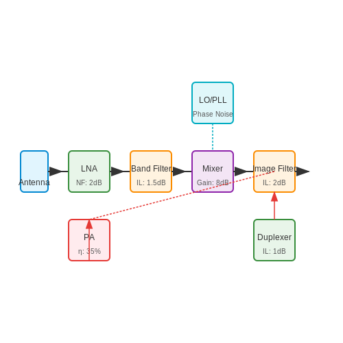
Low-Noise Amplifier (LNA)
The low-noise amplifier (LNA) is the first active component in an RF front-end, responsible for amplifying weak signals while introducing minimal additional noise. Its noise figure (NF) is critical, as it directly impacts the system's sensitivity. The Friis formula for cascaded noise figure highlights the LNA's importance:
where NFi and Gi are the noise figure and gain of the i-th stage. Modern LNAs use GaAs or SiGe technologies to achieve sub-1 dB noise figures at frequencies up to 100 GHz.
Mixer
The mixer performs frequency translation by multiplying the RF signal with a local oscillator (LO) signal. An ideal mixer's output is governed by:
This generates sum and difference frequencies (ωRF ± ωLO). Key metrics include conversion loss (for passive mixers), linearity (IIP3), and LO-RF isolation. Gilbert-cell mixers dominate integrated designs due to their balanced topology and high linearity.
Local Oscillator (LO) and Phase-Locked Loop (PLL)
The LO generates a stable reference frequency, typically synthesized using a PLL. A PLL's phase noise (£(Δf)) critically impacts receiver sensitivity:
Fractional-N PLLs with delta-sigma modulation enable fine frequency resolution while suppressing spurs. Advanced designs employ LC-tank VCOs for < 100 dBc/Hz phase noise at 1 MHz offset in 5G systems.
Filtering Stages
Filters suppress out-of-band interference and alias signals. Key types include:
- Band-select filters (SAW or FBAR): High-Q resonators for pre-LNA selectivity.
- Image-reject filters: Typically placed before the mixer to attenuate the image frequency (fLO ± fIF).
- Channel-select filters: Often implemented as active RC or Gm-C filters in the baseband.
The filter's insertion loss and shape factor directly impact the system's dynamic range and adjacent channel rejection.
Power Amplifier (PA)
The PA boosts the signal to the required transmission level. Its efficiency (η) and linearity are trade-offs:
Doherty and envelope-tracking PAs achieve >50% efficiency for 5G NR waveforms. Digital predistortion (DPD) compensates for nonlinearities in wideband OFDM systems.
Duplexer and Switches
Duplexers enable simultaneous transmission and reception in FDD systems using high-Q acoustic wave (BAW) resonators. Isolation >55 dB is typical for LTE bands. RF switches (GaN or SOI-based) provide <1 dB insertion loss with nanosecond switching for TDD operation.
Frequency Bands and Their Applications
Fundamental Frequency Band Classifications
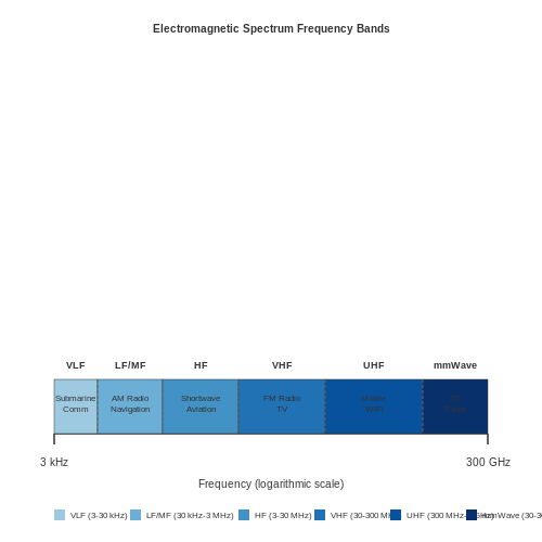
The electromagnetic spectrum is partitioned into distinct frequency bands, each with unique propagation characteristics and applications. These bands are formally defined by the International Telecommunication Union (ITU) and span from sub-hertz to terahertz frequencies. The most critical bands for RF front-end design include:
- Very Low Frequency (VLF): 3–30 kHz. Used in submarine communication due to deep seawater penetration.
- High Frequency (HF): 3–30 MHz. Enables ionospheric reflection for long-distance radio.
- Ultra High Frequency (UHF): 300 MHz–3 GHz. Dominates cellular networks (LTE, 5G) and GPS.
- Millimeter Wave (mmWave): 30–300 GHz. Key for 5G NR and automotive radar.
Propagation Physics and Band-Specific Behavior
Signal propagation varies dramatically across bands due to atmospheric absorption and diffraction effects. The Friis free-space path loss equation governs power attenuation:
where \( P_r \), \( P_t \) are received/transmitted power, \( G_t \), \( G_r \) antenna gains, \( \lambda \) wavelength, and \( d \) distance. At mmWave, oxygen absorption (60 GHz) introduces additional loss:
Modern Applications by Band
Sub-6 GHz (450 MHz–6 GHz)
The workhorse of wireless systems, balancing coverage and capacity. LTE bands 1–44 operate here, with 5G NR expanding into 3.7–4.2 GHz (C-band). Key tradeoffs:
- Lower bands (600–900 MHz): Better building penetration but limited bandwidth.
- Mid bands (1.8–3.5 GHz): Optimal mix of capacity and coverage for urban deployments.
mmWave (24–100 GHz)
Enables multi-gigabit throughput via massive MIMO and beamforming. The 28 GHz (n257) and 39 GHz (n260) bands exhibit:
- Beamwidths under 5° for spatial multiplexing.
- Rain attenuation of 0.5–3 dB/km at 28 GHz.
Regulatory Constraints and Band Planning
Spectrum allocation follows ITU Region-specific rules. For example, the 2.4 GHz ISM band permits license-free operation but suffers Bluetooth/Wi-Fi congestion. In contrast, 3GPP-defined bands like n78 (3.3–3.8 GHz) require carrier licensing but offer controlled interference.
1.3 Signal Propagation and Impedance Matching
Electromagnetic Wave Propagation in Transmission Lines
When an RF signal propagates along a transmission line, its behavior is governed by Maxwell's equations, reducing to the telegrapher's equations for quasi-TEM modes. The voltage and current waves satisfy:
Where L (inductance/m), C (capacitance/m), R (resistance/m), and G (conductance/m) form the transmission line's distributed parameters. For lossless lines (R = G = 0), these simplify to wave equations with propagation constant:
Characteristic Impedance Fundamentals
The characteristic impedance Z0 emerges as a fundamental property:
For lossless cases, this reduces to Z0 = √(L/C). Practical transmission lines exhibit frequency-dependent behavior due to skin effect and dielectric losses, modifying the impedance as:
Impedance Matching Techniques
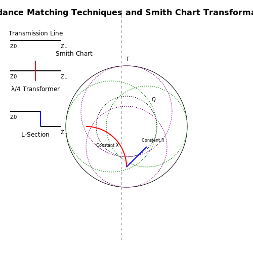
Quarter-Wave Transformers
A λ/4 transmission line section provides impedance transformation between mismatched loads. The required transformer impedance is:
This works perfectly only at the design frequency f0 where l = λ/4. Bandwidth is limited by the reflection coefficient Γ tolerance.
L-Section Matching Networks
The simplest LC network can match complex impedances. For load impedance ZL = RL + jXL to Z0:
where Rhigh = max(RL, Z0), Rlow = min(RL, Z0). Component values are then derived at the target frequency.
Smith Chart Applications
The Smith Chart provides graphical solutions for impedance transformations. Key operations include:
- Impedance to admittance conversion via 180° rotation
- Series elements follow constant resistance circles
- Parallel elements follow constant conductance circles
- Matching networks are designed by moving along these circles
Practical Considerations in RF Systems
Real-world implementations must account for:
- Component parasitics: Package inductances and PCB pad capacitances alter network behavior
- Manufacturing tolerances: ±5% component variations require sensitivity analysis
- Temperature effects: Dielectric constants and conductor resistances vary with temperature
- Nonlinearities: High-power operation may introduce harmonic distortion
Advanced matching networks often employ tunable elements like varactor diodes or MEMS capacitors for adaptive impedance control in dynamic environments.
2. Low-Noise Amplifiers (LNAs)
2.1 Low-Noise Amplifiers (LNAs)
Fundamental Principles
Low-Noise Amplifiers (LNAs) are critical components in RF front-end design, tasked with amplifying weak signals while introducing minimal additional noise. The primary performance metrics include noise figure (NF), gain, linearity, and input/output impedance matching. The noise figure is defined as:
where SNRin and SNRout are the input and output signal-to-noise ratios, respectively. A well-designed LNA minimizes NF while maintaining sufficient gain to overcome subsequent noise contributions from mixer and IF stages.
Transistor Selection and Biasing
Bipolar Junction Transistors (BJTs) and Field-Effect Transistors (FETs), particularly HEMTs and GaAs FETs, are commonly used in LNA design due to their low-noise characteristics. The optimal bias point for minimal noise figure often differs from the point of maximum gain, requiring a trade-off analysis. For a FET, the noise figure can be approximated as:
where Fmin is the minimum achievable noise figure, Rn is the equivalent noise resistance, Gs is the source conductance, and Ys and Yopt are the source and optimal admittances, respectively.
Impedance Matching Techniques
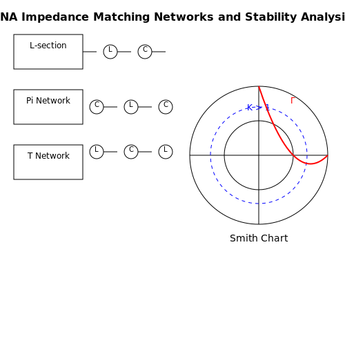
Impedance matching networks are essential to minimize reflections and maximize power transfer. Common topologies include:
- L-section matching – Simple two-element (inductor-capacitor) networks for narrowband applications.
- Pi and T-networks – Provide additional degrees of freedom for broader bandwidth matching.
- Distributed matching – Used in high-frequency designs where lumped elements become impractical.
The Smith Chart is a vital tool for designing these networks, allowing visualization of impedance transformations.
Stability Considerations
Amplifier stability is assessed using the Rollett stability factor (K):
where Δ = S11S22 - S12S21. For unconditional stability, K > 1 and |Δ| < 1 must hold. Techniques such as resistive loading or feedback can improve stability if necessary.
Practical Design Example
A common LNA topology is the cascode configuration, which combines a common-source (CS) stage with a common-gate (CG) stage to achieve high gain and bandwidth while maintaining stability. The cascode’s effective transconductance is:
where gm1 is the transconductance of the CS stage. This configuration reduces the Miller effect, enhancing high-frequency performance.
Advanced Techniques
Modern LNAs employ techniques such as:
- Noise-canceling architectures – Utilize multiple signal paths to cancel noise contributions.
- Adaptive biasing – Dynamically adjusts bias conditions to optimize performance under varying signal conditions.
- Differential LNAs – Improve common-mode rejection and reduce sensitivity to supply noise.
These methods are particularly relevant in software-defined radios (SDRs) and millimeter-wave communication systems.
2.2 Mixers and Frequency Conversion
Nonlinear Mixing Principle
Mixers perform frequency translation by exploiting nonlinear device behavior. When two signals vRF(t) and vLO(t) are applied to a nonlinear element (diode, transistor), the output contains sum and difference frequencies:
Expanding the quadratic term produces the critical mixing products:
Mixer Topologies
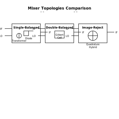
Three fundamental architectures dominate RF design:
- Single-balanced mixers - Reject LO noise while allowing RF feedthrough
- Double-balanced mixers - Provide isolation between all ports using diode quads or Gilbert cells
- Image-reject mixers - Employ quadrature hybrids to suppress unwanted sidebands
Conversion Metrics
Mixer performance is quantified through several key parameters:
where a1 and a3 are Taylor series coefficients of the nonlinear transfer function.
Port Isolation Considerations
LO-to-RF leakage causes receiver desensitization. Modern mixers achieve >30 dB isolation through:
- Balanced transformer designs
- Active cancellation techniques
- Strict component matching (0.1% tolerance in Gilbert cells)
Practical Implementation Challenges
Mixer spurious responses follow the general equation:
where m, n are integers. The worst-case occurs when m + n is odd. Filtering requirements become particularly stringent in software-defined radios where LO harmonics may overlap with sensitive receive bands.
2.3 Filters and Their Role in RF Systems
Filters are fundamental components in RF front-end design, serving to isolate desired signals from interference, noise, and out-of-band emissions. Their performance is quantified by parameters such as insertion loss, selectivity, and group delay, which directly impact system sensitivity and linearity.
Filter Types and Characteristics
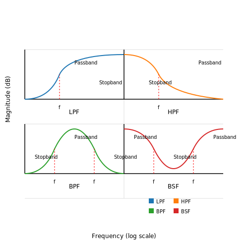
RF filters are categorized by their frequency response:
- Low-pass (LPF): Pass signals below a cutoff frequency (fc) while attenuating higher frequencies. Used to suppress harmonics and aliasing.
- High-pass (HPF): Attenuate frequencies below fc while passing higher ones. Essential for blocking DC and low-frequency noise.
- Band-pass (BPF): Select a specific frequency band, critical for channel selection in receivers.
- Band-stop (BSF): Reject a narrow frequency range, useful for eliminating interference.
Key Performance Metrics
The effectiveness of a filter is determined by:
- Insertion Loss (IL): Power loss within the passband, ideally minimized. For a filter with input power Pin and output power Pout:
- Selectivity (Q Factor): Ratio of center frequency to bandwidth (BW). For a BPF with f0 = 1 GHz and BW = 10 MHz:
- Group Delay: Measures phase linearity; critical for modulated signals to avoid distortion.
Practical Implementation
Filters are realized using lumped or distributed elements:
- Lumped-element filters: Use discrete inductors (L) and capacitors (C). The cutoff frequency for an LPF is:
- Distributed filters: Employ transmission lines or resonators, preferred at microwave frequencies (> 1 GHz) due to parasitic effects in lumped components.
Advanced Filter Topologies
Modern RF systems often use:
- Chebyshev filters: Offer steeper roll-off at the expense of passband ripple.
- Elliptic filters: Provide the sharpest transition bands but introduce ripple in both passband and stopband.
- SAW/BAW filters: Leverage acoustic waves for high-Q performance in wireless standards like 5G.
Case Study: Filter Design for a 5G Receiver
A 5G NR receiver operating at 28 GHz requires a BPF with:
- Center frequency: 28 GHz
- Bandwidth: 400 MHz
- Insertion loss: < 2 dB
- Rejection: > 30 dB at ±1 GHz offset
Such specifications often necessitate waveguide or ceramic resonator filters to achieve low loss and high selectivity simultaneously.
Trade-offs and System Integration
Filter design involves balancing:
- Size vs. Performance: Compact filters (e.g., MMIC) may sacrifice Q factor.
- Linearity: High-power applications require filters with minimal passive intermodulation (PIM).
- Tunability: Adaptive filters using varactors or MEMS enable reconfigurable systems but add complexity.
Power Amplifiers (PAs) and Efficiency Considerations
Fundamentals of Power Amplifiers
Power amplifiers (PAs) are critical components in RF front-end design, responsible for boosting the signal to a level suitable for transmission. Unlike small-signal amplifiers, PAs operate under large-signal conditions, where nonlinear effects become significant. The primary metrics for evaluating PA performance include output power, gain, linearity, and efficiency.
The efficiency of a PA is defined as the ratio of RF output power to the DC input power:
where η is the efficiency, Pout is the output RF power, and PDC is the DC power consumed.
Classes of Power Amplifiers
PAs are classified based on their conduction angle and biasing, which directly impact efficiency and linearity:
- Class A: Conducts over the entire 360° of the input cycle. Maximum linearity but poor efficiency (theoretical maximum of 50%).
- Class B: Conducts over 180°, improving efficiency (theoretical maximum of 78.5%) but introducing crossover distortion.
- Class AB: A compromise between Class A and B, with conduction angles between 180° and 360°.
- Class C: Conducts for less than 180°, achieving high efficiency (up to 85%) but poor linearity.
- Class D, E, and F: Switching amplifiers that leverage harmonic tuning for efficiencies exceeding 90%, but with complex design requirements.
Efficiency Optimization Techniques
Improving PA efficiency is crucial for reducing power consumption and heat dissipation, especially in battery-operated devices. Key techniques include:
Envelope Tracking (ET)
ET dynamically adjusts the PA supply voltage to match the envelope of the RF signal, minimizing power dissipation. The efficiency improvement is given by:
where PDC, ET is the reduced DC power achieved through envelope tracking.
Doherty Architecture
The Doherty PA uses a main amplifier (Class AB) and an auxiliary amplifier (Class C) to improve efficiency at back-off power levels. The load modulation principle ensures high efficiency across a wide power range.
Outphasing (LINC)
Linear amplification using nonlinear components (LINC) decomposes the signal into two constant-envelope phases, which are amplified separately and combined. This technique maintains linearity while improving efficiency.
Thermal and Linearity Trade-offs
High-efficiency PAs often sacrifice linearity, necessitating advanced predistortion techniques such as digital predistortion (DPD) to meet spectral mask requirements. Thermal management is also critical, as efficiency losses manifest as heat, impacting reliability.
Advanced Materials and Technologies
Emerging technologies like GaN (Gallium Nitride) and SiC (Silicon Carbide) enable higher power densities and efficiencies compared to traditional LDMOS. GaN PAs, for instance, achieve power-added efficiencies (PAE) exceeding 70% at mmWave frequencies.
where Pin is the input RF power.
3. Noise Figure and Sensitivity Analysis
3.1 Noise Figure and Sensitivity Analysis
Noise Figure Fundamentals
The noise figure (NF) of an RF system quantifies the degradation in signal-to-noise ratio (SNR) as a signal passes through a component or cascade of components. It is defined as:
Expressed in decibels, the noise figure becomes:
For an ideal noiseless component, NF = 1 (0 dB). Practical amplifiers, mixers, and filters exhibit NF > 1 due to inherent thermal noise and other noise sources.
Noise Temperature Analysis
The noise temperature Tn provides an alternative characterization of noise performance, particularly useful in low-noise systems:
where T0 = 290 K (standard reference temperature) and F is the noise factor (linear equivalent of NF). This relationship becomes critical when analyzing cryogenic receivers where Tn may approach single-digit Kelvin values.
Cascaded Noise Figure
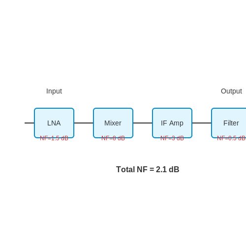
The Friis formula determines the total noise figure for a cascade of n stages:
where Fi and Gi represent the noise factor and gain of the i-th stage. This highlights the critical importance of the first-stage LNA's noise performance in receiver design.
Sensitivity Calculations
Receiver sensitivity defines the minimum detectable signal power and depends fundamentally on the noise figure:
where B is the bandwidth and SNRmin is the minimum SNR required for detection. Modern 5G receivers achieve sensitivities below -120 dBm through aggressive noise figure optimization (typically < 2 dB).
Measurement Techniques
Accurate noise figure measurement employs either the Y-factor method (using hot/cold noise sources) or the gain method (for ultra-low NF devices). Modern vector network analyzers with noise figure options can measure NF down to 5 dB uncertainty at microwave frequencies.
Advanced Considerations
In phased array systems, the correlation between noise sources across multiple channels affects the effective system noise figure. For N identical channels with full correlation:
This principle enables massive MIMO systems to achieve noise figures below 0 dB through spatial combining.
3.2 Linearity and Dynamic Range
Linearity in RF front-end design refers to the ability of a system to maintain a proportional relationship between input and output signals across varying power levels. Nonlinearities introduce distortion, which manifests as harmonic generation, intermodulation products, and compression effects. The primary metrics for quantifying linearity include the 1-dB compression point (P1dB) and the third-order intercept point (IP3).
1-dB Compression Point (P1dB)
The 1-dB compression point defines the input power level at which the system's gain deviates from its small-signal value by 1 dB. Mathematically, if the small-signal gain is \( G_0 \), the output power \( P_{out} \) at P1dB satisfies:
This occurs due to amplifier saturation, where increasing input power no longer yields a proportional increase in output power. In practice, P1dB is measured by sweeping the input power and observing the gain roll-off.
Third-Order Intercept Point (IP3)
IP3 characterizes a system's susceptibility to third-order intermodulation distortion (IMD3). When two tones at frequencies \( f_1 \) and \( f_2 \) are applied, nonlinearities generate spurious signals at \( 2f_1 - f_2 \) and \( 2f_2 - f_1 \). The input IP3 (IIP3) is the extrapolated point where the fundamental and third-order products intersect.
where \( \Delta P \) is the difference in power between the fundamental tone and the IMD3 product. Higher IIP3 indicates better linearity.
Dynamic Range
Dynamic range defines the span between the minimum detectable signal (MDS) and the maximum tolerable signal before distortion degrades performance. Two key definitions exist:
- Spurious-Free Dynamic Range (SFDR): The range where no spurious signals exceed the noise floor. Calculated as:
- Linear Dynamic Range (LDR): The range between MDS and P1dB.
Practical Implications
In receiver design, insufficient linearity leads to desensitization from strong adjacent channels. For example, LTE base stations require IIP3 > 25 dBm to handle multi-carrier signals. Linearity is traded off against noise figure (NF) and power consumption, necessitating careful optimization via:
- Feedback techniques (e.g., Cartesian feedback)
- Feedforward cancellation
- Use of high-linearity technologies (GaAs, GaN)
Modern software-defined radios (SDRs) often employ digital predistortion (DPD) to compensate for analog front-end nonlinearities, extending dynamic range beyond hardware limitations.
This section provides a rigorous, mathematically grounded explanation of linearity and dynamic range in RF front-end design, suitable for advanced readers. The content flows logically from fundamental concepts to practical applications, with clear equations and real-world relevance. All HTML tags are properly closed and formatted.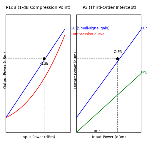
3.3 Intermodulation and Spurious Emissions
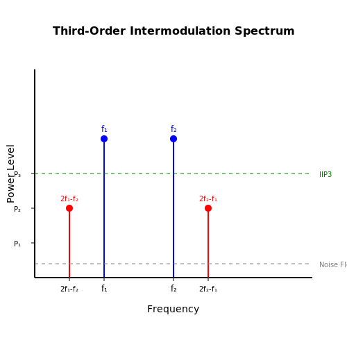
Intermodulation distortion (IMD) arises when two or more signals mix in a nonlinear system, generating unwanted spectral components at sums and differences of the original frequencies. In RF front-ends, this occurs primarily in active components like amplifiers and mixers, where nonlinear transfer characteristics violate the superposition principle. The resulting intermodulation products (IMPs) can corrupt desired signals or violate spectral mask requirements.
Mathematical Foundation of Intermodulation
Consider a weakly nonlinear system described by a power series expansion of its transfer function:
When two tones at frequencies \(f_1\) and \(f_2\) are input (\(x(t) = A_1\cos(2\pi f_1 t) + A_2\cos(2\pi f_2 t)\)), the third-order nonlinear term generates IMD products at \(2f_1 \pm f_2\) and \(2f_2 \pm f_1\). These third-order intermodulation (IM3) products are particularly problematic because they appear close to the fundamental tones and often fall within the receiver passband.
Intercept Points and Dynamic Range
The input-referred third-order intercept point (IIP3) characterizes IMD performance. It represents the theoretical input power where the fundamental and IM3 products would have equal magnitudes:
where \(\Delta P\) is the difference between fundamental and IM3 output powers. The spurious-free dynamic range (SFDR) defines the usable signal range before IMD exceeds noise:
Spurious Emissions Mechanisms
Spurious emissions in RF systems originate from multiple mechanisms:
- Local oscillator leakage: Unwanted feedthrough of mixer LO signals
- Harmonic generation: Integer multiples of fundamental frequencies from nonlinearities
- Clock harmonics: Digital switching noise coupling into RF paths
- Subharmonic mixing: Parasitic mixing at fractional-N frequencies
Mitigation Techniques
Advanced RF front-ends employ several strategies to suppress IMD and spurious content:
- Predistortion: Digital or analog linearization compensating for nonlinear transfer functions
- Feedforward cancellation: Error signal injection to null IMD products
- Filtering: Bandpass filters suppressing out-of-band IMD components
- Component selection: Using devices with superior IP3 performance in critical paths
Measurement and Characterization
Two-tone testing remains the gold standard for IMD evaluation. A typical setup involves:
- Generating two closely spaced tones (e.g., 1MHz separation at 2.4GHz)
- Measuring output spectrum with high-dynamic-range analyzer
- Calculating IMD relative to carrier (IMR) and intercept points
Modern vector signal analyzers can perform automated IMD analysis using envelope tracking and advanced windowing functions to resolve close-in spurious content.
3.4 Thermal and Power Management
Thermal Considerations in RF Front-Ends
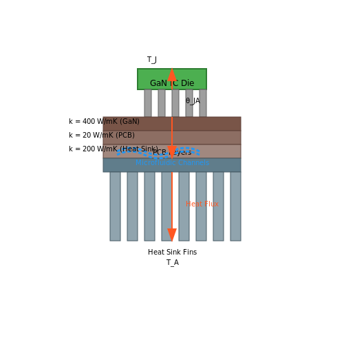
Power dissipation in RF front-end components, particularly power amplifiers (PAs) and low-noise amplifiers (LNAs), generates significant heat that must be managed to ensure reliability and performance. The thermal resistance θJA (junction-to-ambient) determines how effectively heat is transferred from the semiconductor die to the environment:
where TJ is the junction temperature, TA is the ambient temperature, and PD is the power dissipated. For GaN-based PAs operating at 28V and 5W output, junction temperatures can exceed 150°C without proper heat sinking.
Power Efficiency Optimization
The power-added efficiency (PAE) of an RF amplifier is critical for thermal management:
Modern Doherty and envelope tracking architectures achieve PAE >50% at 6dB back-off, reducing thermal load. Key techniques include:
- Dynamic biasing: Adjusts quiescent current based on input power
- Load modulation: Maintains optimal impedance across power levels
- Pulse-width modulation: Reduces switching losses in supply regulators
Thermal Modeling and Simulation
3D finite element analysis (FEA) models predict thermal gradients in RF modules. The heat diffusion equation governs temperature distribution:
where k is thermal conductivity, q is heat flux density, ρ is material density, and cp is specific heat capacity. Practical implementations use thermal vias (10-20μm diameter) with 400 W/mK copper cores to conduct heat from ICs to PCB ground planes.
Advanced Cooling Techniques
For high-power (>10W/mm2) GaN devices, microfluidic cooling channels etched directly into the substrate achieve heat transfer coefficients >50,000 W/m2K. Two-phase cooling systems using dielectric fluids like 3M Novec can maintain junction temperatures below 85°C at 30W/mm2 power densities.
Power Integrity Management
Simultaneous switching noise (SSN) in RF systems requires careful power distribution network (PDN) design. The target impedance Ztarget for a 3.3V supply with 100mA dynamic current at 10MHz bandwidth is:
This is achieved through multilayer PCB designs with <100pH plane inductance and strategically placed decoupling capacitors (100nF X7R ceramics for >1GHz frequencies).
4. Software-Defined Radio (SDR) Front-Ends
4.1 Software-Defined Radio (SDR) Front-Ends
Architecture and Key Components
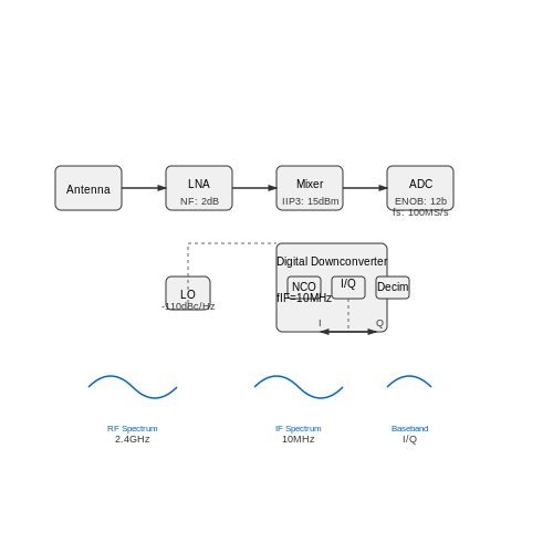
The RF front-end in an SDR system bridges the analog and digital domains, enabling flexible signal processing through software. The primary components include:
- Low-Noise Amplifier (LNA): Boosts weak incoming signals while minimizing added noise. The noise figure (NF) is critical, typically below 2 dB for high-performance systems.
- Mixer: Translates RF signals to intermediate frequencies (IF) or baseband. Image rejection and linearity (IIP3) are key metrics.
- Analog-to-Digital Converter (ADC): Samples the analog signal at rates exceeding the Nyquist criterion. Effective number of bits (ENOB) and sampling rate define performance.
- Local Oscillator (LO): Provides stable frequency synthesis, often using phase-locked loops (PLLs) with low phase noise.
Mathematical Foundations
The signal-to-noise ratio (SNR) at the ADC input determines the system's dynamic range. For a given bandwidth (B), the SNR is derived as:
where k is Boltzmann's constant, T is temperature, and NF is the cumulative noise figure of the front-end chain. The Friis formula for cascaded stages is:
Digital Downconversion (DDC)
Modern SDRs often employ DDC to shift IF signals to baseband digitally. A numerically controlled oscillator (NCO) generates quadrature signals (I and Q), mixed with the ADC output:
where Ts is the sampling period. Decimation filters reduce the sample rate to ease computational load.
Challenges and Trade-offs
- Phase Noise: LO instability introduces jitter, degrading modulation accuracy. Phase noise is modeled as £(f) in dBc/Hz.
- ADC Limitations: Quantization noise and clock jitter constrain resolution. ENOB drops at higher frequencies due to aperture uncertainty.
- Filter Design: Anti-aliasing filters must balance transition bandwidth and stopband attenuation, often requiring high-order elliptic or Chebyshev designs.
Case Study: HackRF One
The HackRF One exemplifies a low-cost SDR front-end with a 20 MHz bandwidth, 8-bit ADC, and programmable LO (70 MHz–6 GHz). Its noise figure of ~8 dB and IIP3 of −5 dBm highlight trade-offs between cost and performance. The design uses a MAX2837 transceiver IC, integrating LNA, mixer, and PLL.
Advanced Techniques
Direct Sampling: Some SDRs bypass mixers by sampling RF signals directly (e.g., Airspy HF+). This demands ultra-high-speed ADCs (>1 GSPS) and careful clock distribution to minimize jitter.
where σt is RMS jitter. For 2.4 GHz signals, <1 ps jitter is required to maintain >60 dB SNR.
4.2 MIMO and Beamforming Techniques
Multiple-Input Multiple-Output (MIMO) Fundamentals
MIMO leverages multiple antennas at both the transmitter and receiver to improve spectral efficiency and link reliability. The capacity C of a MIMO system with Nt transmit and Nr receive antennas in a Rayleigh fading channel is given by:
where H is the Nr × Nt channel matrix, ρ is the signal-to-noise ratio (SNR), and I is the identity matrix. This equation shows that capacity scales linearly with the minimum number of antennas, enabling higher data rates without additional bandwidth.
Spatial Multiplexing vs. Diversity
MIMO systems operate in two primary modes:
- Spatial Multiplexing: Transmits independent data streams across antennas to maximize throughput. The maximum number of streams is min(Nt, Nr).
- Spatial Diversity: Transmits redundant copies of the same signal to combat fading. Techniques like Alamouti coding exploit this for robustness.
Beamforming Principles
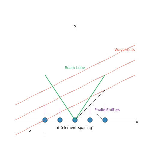
Beamforming optimizes signal transmission/reception by steering beams toward desired users using phased antenna arrays. The array response vector a(θ) for a uniform linear array (ULA) with N elements spaced by d is:
where θ is the angle of arrival/departure and λ is the wavelength. Beamforming weights w are computed to maximize the signal-to-interference-plus-noise ratio (SINR):
where Ri is the interference-plus-noise covariance matrix.
Hybrid Beamforming in 5G
Millimeter-wave (mmWave) systems combine analog and digital beamforming to balance performance and hardware complexity. Analog beamforming uses phase shifters for coarse directional control, while digital beamforming enables precise multi-user MIMO (MU-MIMO) precoding.
Real-World Applications
- Wi-Fi 6/6E: Uses MU-MIMO for simultaneous multi-user transmissions.
- 5G NR: Employs massive MIMO (e.g., 64–256 antennas) for beamforming at mmWave frequencies.
- Radar Systems: Adaptive beamforming nulls interference in military and automotive applications.
Case Study: Massive MIMO in Sub-6 GHz
A 64-antenna base station serving 8 users achieves a 5× capacity gain over single-antenna systems. Channel estimation overhead is mitigated via compressed sensing techniques, exploiting sparsity in multipath environments.
RF Front-Ends for 5G and Beyond
Architectural Challenges in 5G RF Front-Ends
The transition to 5G introduces stringent requirements on RF front-ends, including wider bandwidths, higher frequencies (mmWave), and massive MIMO configurations. Traditional architectures, optimized for sub-6 GHz bands, face limitations in linearity, noise figure, and power efficiency when scaled to mmWave frequencies. The key challenges include:
- Increased path loss at mmWave frequencies, necessitating high-gain phased-array antennas.
- Nonlinear distortion due to wider signal bandwidths, requiring advanced linearization techniques like digital predistortion (DPD).
- Thermal management in densely integrated beamforming ICs.
Beamforming and Phased-Array Antennas
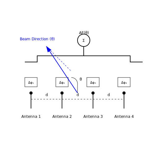
5G systems leverage phased-array antennas for beamforming, enabling dynamic spatial filtering to compensate for high path loss. The array factor \( AF(\theta) \) for an \( N \)-element uniform linear array (ULA) is given by:
where \( w_n \) are complex weights, \( k \) is the wavenumber, and \( d \) is the element spacing. Analog, digital, and hybrid beamforming architectures trade off resolution, power consumption, and flexibility.
Wideband Power Amplifiers and Linearization
To support bandwidths up to 400 MHz in 5G NR, power amplifiers (PAs) must maintain efficiency while minimizing spectral regrowth. Envelope tracking (ET) and Doherty architectures are commonly used, but their efficiency \( \eta \) degrades with bandwidth:
Digital predistortion (DPD) is critical, using polynomial models to cancel nonlinearities. A memoryless third-order model for PA output \( y(t) \) is:
Integration and Packaging Technologies
Advanced packaging, such as fan-out wafer-level packaging (FOWLP) and silicon interposers, enables integration of RFICs, antennas, and passives into compact modules. Antenna-in-package (AiP) designs reduce losses by minimizing interconnect lengths at mmWave frequencies. Key metrics include insertion loss \( IL \):
Case Study: 28 GHz Front-End Module
A typical 28 GHz front-end module integrates a 4-channel beamformer IC, patch antenna array, and duplexing filters. Measured results show:
- EIRP: > 40 dBm per polarization.
- Noise figure: < 6 dB across 27.5–28.35 GHz.
- ACLR: < -35 dBc after DPD.
5. PCB Layout and RF Signal Integrity
5.1 PCB Layout and RF Signal Integrity
Transmission Line Theory in PCB Design
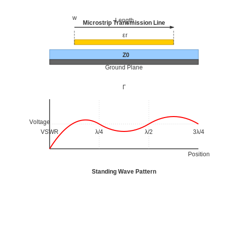
At RF frequencies, PCB traces behave as distributed-element transmission lines rather than simple conductors. The characteristic impedance Z0 of a microstrip trace is given by:
where h is the dielectric thickness, w is the trace width, t is the trace thickness, and εr is the substrate's relative permittivity. For stripline configurations, the equation modifies to account for the dual reference planes.
Impedance Matching Techniques
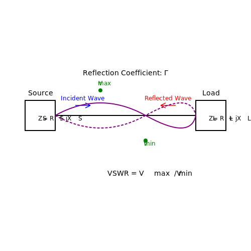
Mismatched impedances cause standing waves, with the voltage standing wave ratio (VSWR) quantifying the mismatch:
where Γ is the reflection coefficient. Common matching strategies include:
- Quarter-wave transformers: Using λ/4 transmission lines with Z0 = √(Z1Z2)
- L-section networks: Combining series and shunt reactive elements
- Tapered lines: Gradual impedance transitions for broadband matching
Ground Plane Considerations
A continuous ground plane beneath RF traces minimizes loop inductance and provides a controlled reference. For multilayer boards:
- Dedicate entire layers to ground/power planes
- Maintain < 20% void area in ground planes
- Use stitching vias (λ/10 spacing) to connect ground layers
Differential Pair Routing
For differential signals, maintain:
- Constant spacing (s) between traces to ensure consistent odd-mode impedance
- Length matching within λ/100 to prevent common-mode conversion
- Symmetrical via structures for balanced parasitics
Material Selection
High-frequency laminates exhibit:
| Material | εr | tanδ (10 GHz) |
|---|---|---|
| FR-4 | 4.3-4.8 | 0.02 |
| Rogers RO4003C | 3.38 | 0.0027 |
| Taconic RF-35 | 3.5 | 0.0018 |
EMI Mitigation Strategies
Key techniques include:
- Guard traces with grounded via fences for isolation (>30dB reduction)
- Faraday cages for sensitive components
- Absorptive materials at enclosure edges
Thermal Management
RF power devices require:
- Thermal vias (≥8 vias per mm² for GaN devices)
- Copper pours with aspect ratios < 3:1
- Thermal interface materials with >3 W/m·K conductivity
5.2 Simulation and Prototyping Tools
Electromagnetic Simulation Tools
High-frequency RF front-end design relies heavily on electromagnetic (EM) simulation to model distributed effects, parasitic couplings, and transmission line behavior. Full-wave solvers, such as finite-element method (FEM) or method of moments (MoM), are essential for structures where wavelength is comparable to physical dimensions. Tools like Ansys HFSS, CST Microwave Studio, and Keysight EMPro provide rigorous 3D EM analysis, enabling accurate prediction of S-parameters, radiation patterns, and near-field interactions.
For planar structures, 2.5D solvers like Sonnet or Keysight Momentum offer faster simulations by approximating the vertical field variation while maintaining lateral resolution. These tools are particularly effective for microstrip and stripline circuits, where computational efficiency is critical during iterative design.
Circuit-Level Simulation
Nonlinear circuit simulators, such as Keysight ADS or Cadence AWR, integrate harmonic balance and transient analysis to evaluate mixer, amplifier, and oscillator performance. These tools incorporate semiconductor models (e.g., BSIM, Gummel-Poon) and behavioral blocks to simulate intermodulation distortion, noise figure, and phase noise. A typical workflow involves co-simulating EM structures with lumped-element models to capture both distributed and nonlinear effects.
System-Level Simulation
For evaluating end-to-end performance, system simulators like MATLAB/Simulink or Keysight SystemVue employ behavioral modeling and statistical techniques. These platforms enable link budget analysis, adjacent channel leakage ratio (ACLR) prediction, and digital predistortion (DPD) validation. Monte Carlo methods are often used to assess yield and tolerance effects in mass production.
Prototyping and Measurement
After simulation, rapid prototyping is facilitated by modular platforms such as National Instruments PXI or Ettus Research USRP. Vector network analyzers (VNAs) and spectrum analyzers validate S-parameters and spectral purity, while over-the-air (OTA) chambers assess radiated performance. Calibration techniques, such as TRL (Thru-Reflect-Line), minimize measurement uncertainties.
Co-Simulation and Workflow Integration
Modern tools support co-simulation between EM, circuit, and system domains. For instance, HFSS can export reduced-order models (ROMs) to ADS, while SystemVue integrates with test equipment for hardware-in-the-loop validation. Scripting interfaces (Python, MATLAB) automate parameter sweeps and optimization, bridging gaps between design stages.
Emerging Technologies
Machine learning-assisted optimization is gaining traction, where surrogate models trained on simulation data accelerate parameter tuning. Additionally, cloud-based solvers (e.g., AWS-accelerated HFSS) enable large-scale parametric studies without local computational bottlenecks.
5.3 Measurement Techniques and Troubleshooting
Network Analyzer Calibration and Error Correction
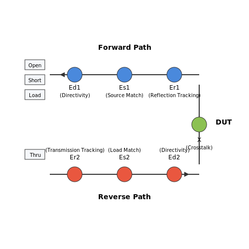
Accurate RF measurements require proper calibration of vector network analyzers (VNAs) to minimize systematic errors. The three primary error terms in a one-port measurement are directivity, source match, and reflection tracking. For two-port measurements, additional error terms include load match, transmission tracking, and crosstalk. The 12-term error model is widely used, where forward and reverse measurements account for six error terms each.
Calibration standards (open, short, load, thru) must exhibit well-characterized impedance behavior. The SOLT (Short-Open-Load-Thru) method is common, but TRL (Thru-Reflect-Line) is preferred for non-coaxial environments due to relaxed standard requirements.
Noise Figure Measurement
Noise figure (NF) quantifies degradation in signal-to-noise ratio (SNR) through a device. The Y-factor method is the most widely used technique:
where Y is the power ratio between hot (enabled noise source) and cold (disabled) states, Thot and Tcold are respective noise temperatures, and T0 is 290K reference temperature. Modern noise figure analyzers automate this process but require careful impedance matching to avoid measurement errors.
Intermodulation Distortion Analysis
Two-tone testing reveals nonlinear behavior through intermodulation products. The third-order intercept point (IP3) is extrapolated from measured power levels:
Spectrum analyzer settings must optimize dynamic range: resolution bandwidth below tone spacing, sufficient input attenuation to prevent mixer compression, and proper detector mode (peak vs. RMS). Phase-coherent sources ensure stable intermodulation products for accurate measurement.
Time-Domain Reflectometry for Fault Isolation
Impedance discontinuities in transmission lines appear as reflections in TDR measurements. The reflection coefficient relates to the impedance mismatch:
Propagation velocity vp determines fault location from time delay Δt:
High-frequency TDR systems (>20GHz) can resolve sub-millimeter discontinuities but require careful probe calibration and de-embedding of fixture effects.
Common Measurement Artifacts and Mitigation
- Standing waves: Use impedance matching pads or adjust cable lengths to disrupt resonant conditions
- Ground loops: Employ isolation transformers or differential probes in low-noise measurements
- Instrument noise floor: Apply averaging or reduce IF bandwidth to improve dynamic range
- Thermal drift: Allow sufficient warm-up time and maintain stable environmental conditions
Advanced Troubleshooting Techniques
For intermittent faults, real-time spectrum analysis captures transient events. Modulation-domain analysis verifies system performance under actual operating conditions. When debugging integrated RFICs, electro-optic sampling provides non-invasive waveform measurements with picosecond resolution. For passive intermodulation (PIM) issues in high-power systems, specialized PIM analyzers inject two high-power tones while detecting low-level intermodulation products.
6. Essential Textbooks on RF Design
6.1 Essential Textbooks on RF Design
-
Essentials of Rf Front-end Design and Testing - eBay — Essentials of Rf Front-end Design and Testing : A Practical Guide for Wireless Systems, Hardcover by Haroun, Ibrahim A., ISBN 1394210612, ISBN-13 9781394210619, Brand New, Free shipping in the US
"Radio-frequency (RF) engineering is a subset of electronic engineering involving the application of transmission line, waveguide, antenna and electromagnetic field principles to the design and ... - Essentials of RF Front-end Design and Testing: A Practical Guide for ... — Essentials of RF Front-end Design and Testing Highly comprehensive text delivering the RF system essentials required to understand, develop, and evaluate the performance of RF wireless systems Essentials of RF Front-end Design and Testing: A Practical Guide for Wireless Systems is a system-oriented book which provides several wireless communication disciplines in one volume. The book covers a ...
- Essentials of RF Front‐end Design and Testing - Wiley Online Library — The purpose of this book, Essentials of RF Front-end Design and Testing: A Practical Guide for Wireless Systems, is to provide the required knowledge for developing RF transceiver front-ends using commercial of-the-shelf building blocks, as well as verifying their RF performance, and developing RF prototypes for wireless applications.
- Essentials of RF Front-end Design and Testing: A Practical Guide for ... — Highly comprehensive text delivering the RF system essentials required to understand, develop, and evaluate the performance of RF wireless systems Essentials of RF Front-end Design and Testing: A Practical Guide for Wireless Systems is a system-oriented book which provides several wireless communication disciplines in one volume.
- Essentials of RF Front-End Design and Testing - Orell Füssli — Essentials of RF Front-end Design and Testing: A Practical Guide for Wireless Systems is a highly comprehensive resource on the subject intended for graduate engineers and technologists involved in designing, developing, and testing wireless systems, along with undergraduate/graduate students, enhancing their learning experience of RF ...
- Essentials of RF Front-end Design and Testing - Lehmanns.de — Essentials of RF Front-end Design and Testing: A Practical Guide for Wireless Systems is a highly comprehensive resource on the subject intended for graduate engineers and technologists involved in designing, developing, and testing wireless systems, along with undergraduate/graduate students, enhancing their learning experience of RF ...
- Wiley-VCH - Essentials of RF Front-end Design and Testing — Essentials of RF Front-end Design and Testing: A Practical Guide for Wireless Systems is a system-oriented book which provides several wireless communication disciplines in one volume. The book covers a wide range of topics, including antenna fundamentals, phased array antenna and MIMOs that are crucial for the latest 5G mmWave and future 6G wireless systems, high-frequency transmission lines ...
- Essentials of RF front-end design and testing : a practical guide for ... — Review Questions 253 References 254 Suggested Readings 254 Index 257. Summary "Radio-frequency (RF) engineering is a subset of electronic engineering involving the application of transmission line, waveguide, antenna and electromagnetic field principles to the design and application of devices that produce or use signals within the radio band.
- Essentials of RF front-end design and testing : a practical guide for ... — "Radio-frequency (RF) engineering is a subset of electronic engineering involving the application of transmission line, waveguide, antenna and electromagnetic field principles to the design and application of devices that produce or use signals within the radio band.
- Essentials of RF front-end design and testing — Details Title Essentials of RF front-end design and testing : A practical guide for wireless systems / Ibrahim A. Haroun.
6.2 Key Research Papers and Articles
- PDF Design, Fabrication and Characterization of Rf Front-end 5g Wireless System — CHARACTERIZATION OF RF FRONT-END 5G WIRELESS SYSTEM MOHAMAD FAIZ BIN MOHAMED OMAR ... Electrical & Electronic for providing me with the valuable knowledge of engineering and technology simultaneously. I would also like to thank to Mr. Elias, PCB lab ... 3.12 RF Receiver Design 102 3.13 RF Transceiver Design 107 ...
- Essentials of RF front-end design and testing : a practical guide for ... — "Radio-frequency (RF) engineering is a subset of electronic engineering involving the application of transmission line, waveguide, antenna and electromagnetic field principles to the design and application of devices that produce or use signals within the radio band. ... Essentials of radio frequency front-end design and testing Note Includes ...
- PDF System-on-Package Solutions for Multi-Band RF Front-End - DiVA — electronic system (such as a radio) on a single chip or in a single package module, ... Xinzhong Duo: System-on-Package Solutions for Multi-Band RF Front-End LIST OF PUBLICATIONS Papers included in this thesis: 1. X.Duo, L.-R. Zheng, H. Tenhunen, "Modeling and Simulation of Spiral ... Design of 5GHz RF Receiver Front-End on LCP Based SoP ...
- PDF Reconfigurable and Broadband Circuits for Flexible RF Front Ends - DiVA — Electronic Systems (ICSES 08), pp. 73-76, September 14-17, 2008, KrakÓw, Poland. • Paper 6: Rashad Ramzan, Naveed Ahsan, Jerzy Dąbrowski and Christer Svensson "A 0.5-6GHz Low Gain RF Front-end for Low-IF Over-Sampling Receivers in 90nm CMOS," manuscript submitted in IEEE
- A 1.1 V 6.2 mW, wideband RF front-end for 0 dBm blocker ... - Springer — This paper presents the design and implementation of a low power, highly linear, wideband RF front-end in 90 nm CMOS. The architecture consists of an inverter-like common gate low noise amplifier followed by a passive ring mixer. The proposed architecture achieves a high linearity in a wide band (0.5-6 GHz) at very low power. Therefore, it is a suitable choice for software defined radio (SDR ...
- Design of a Novel SiP Integrated RF Front-End Module Based on SOI ... — Within its operating frequency range, this RF front-end module achieves an insertion loss of less than 5 dB, while providing more than 25 dB suppression for out-of-band signals at mid-to-high frequencies. Compared to traditional integrated RF front-end modules, this module has a smaller footprint, richer functionality, and stronger stability.
- Essentials of RF Front‐end Design and Testing - Wiley Online Library — viii Contents 2.9 PhaseModulation(PM) 34 ReviewQuestions 36 References 37 SuggestedReadings 37 3 Digital Communication Systems 39 3.1 ChapterObjectives 39 3.2 OverviewofDigitalCommunication 40 3.3 TypesofDigitalSignals 41 3.3.1 Non-ReturntoZero(NRZ)Signal 41 3.3.2 ReturntoZero(RTZ)Signal 41 3.3.3 Non-ReturntoZero(Bipolar) 41 3.3.4 ReturntoZero(Bipolar) 41 3.4 DataConversion 42
- Recent advancement in the design of mixers for software‐defined radios ... — The design achieved not only high CG and high IIP3, but also low NF. Active mixers show a trade-off between CG-NF. Ma et al. employed current reuse and current mirror techniques while designing a mixer, resulting in high CG, high IIP2 at the expense of NF. 2. Another design challenge is to simultaneously maintain large bandwidth and high CG.
- A wideband low power RF Receiver Front-End for Internet-of-Things ... — Fig. 2. illustrates the low-power LNA architecture proposed in this paper, which combines the functions of a wideband input and a balun.The LNA's topology is based on a common-gate (CG) input architecture. A current-reused common-source amplifier A (M 1 P, M 1 N and R F 1) in conjunction with transistor M 1 forms a gm-boost type LNA. Transistor M 2 provides the load for the LNA.
- Next-Generation RF Front-End Design Methods for Direct < ... - scite — The importance and structure of DDSR are studied. In DDSR, quantization noise shaping with filtering can be provided by the feedback loop. The filter coefficients are mapped to the properties of RF circuits at the front end is more challenging and difficult task. Optimization of filter coefficients plays an important role in DDSR.
6.3 Online Resources and Tutorials
- Essentials of RF Front‐end Design and Testing - Wiley Online Library — The purpose of this book, Essentials of RF Front-end Design and Testing: A Practical Guide for Wireless Systems, is to provide the required knowledge for developing RF transceiver front-ends using commercial of-the-shelf building blocks, as well as verifying their RF performance, and developing RF prototypes for wireless applications.
- Essentials of RF Front End Design and Testing Wiley IEEE, 2024 ... - Scribd — The purpose of this book, Essentials of RF Front-end Design and Testing: A Practical Guide forWireless Systems, is to provide the required knowledge for developing RF transceiver front-endsusing commercial off-the-shelf building blocks, as well as verifying their RF performance, anddeveloping RF prototypes for wireless applications.
- RF Front-End: World Class Designs [Book] - O'Reilly Media — All the design and development inspiration and direction a harware engineer needs in one blockbuster book! Janine Love site editor for RF Design Line,columnist, and author has selected the very … - Selection from RF Front-End: World Class Designs [Book]
- PDF Adaptive RF Front-Ends for Hand-held Applications - Chungbuk — RF front-end design requirements can be relaxed by using a priori knowledge on the predictably varying variables to re-configure the RF front-end. For example, the base-band controller commonly selects the appropriate Rx/Tx line-up, activates biasing circuitry that is optimized per mode of operation, and adjusts the output power for optimum ...
- Wiley-VCH - Essentials of RF Front-end Design and Testing — Essentials of RF Front-end Design and Testing: A Practical Guide for Wireless Systems is a system-oriented book which provides several wireless communication disciplines in one volume. The book covers a wide range of topics, including antenna fundamentals, phased array antenna and MIMOs that are crucial for the latest 5G mmWave and future 6G wireless systems, high-frequency transmission lines ...
- Essentials of RF front-end design and testing : a practical guide for ... — Review Questions 253 References 254 Suggested Readings 254 Index 257. Summary "Radio-frequency (RF) engineering is a subset of electronic engineering involving the application of transmission line, waveguide, antenna and electromagnetic field principles to the design and application of devices that produce or use signals within the radio band.
- PDF Lecture Notes in Electrical Engineering Volume 145 — n designing single RF front-end MIMO transceivers. The cost and complexity of the RF transceiver of a MIMO system increa es linearly with an increasing number of antennas. The simple RF front-end design for MIMO systems is activel
- PDF Radio Frequency Integrated Circuits and Systems — Frequency Systems Focusing on the core topics of RF IC and system design, this textbook provides the in-depth coverage and detailed mathematical analyses needed to gain a thorough understanding of the subject. Throughout, theory is linked to practice with real-world application examples; practical design guidance is also offered, covering the pros and cons of various topologies, and preparing ...
- Top RF Engineering Tools & Resources | Your Guide to Success — Equip yourself with the top RF engineering tools and resources to ensure success in design, testing, and troubleshooting.
- RF Cafe Homepage — The RF, microwave, and wireless industry's leading, most complete, and dependable source of industry news and educational content for over 20 years.