Waveguide Transmission Lines
1. Basic Principles of Waveguides
Basic Principles of Waveguides
Waveguides are structures that confine and direct electromagnetic waves along a desired path with minimal energy loss. Unlike conventional transmission lines, waveguides rely on boundary conditions to propagate electromagnetic energy rather than voltage and current distributions. The fundamental principle governing waveguide operation stems from solving Maxwell's equations under specific geometric constraints.
Electromagnetic Wave Propagation in Waveguides
The behavior of electromagnetic fields in a waveguide is derived from the vector Helmholtz equation:
where k is the wavenumber. For a rectangular waveguide with dimensions a × b, we assume propagation in the z-direction. The electric and magnetic fields can be decomposed into transverse (T) and longitudinal (L) components:
where γ is the propagation constant. The boundary conditions require that the tangential electric field vanishes at the conducting walls, leading to discrete modes of propagation.
Modes of Propagation
Waveguides support two primary field configurations:
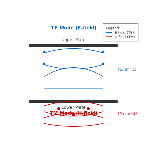
- Transverse Electric (TE) modes: No electric field component in the direction of propagation (Ez = 0)
- Transverse Magnetic (TM) modes: No magnetic field component in the direction of propagation (Hz = 0)
The cutoff frequency for a given mode (m,n) in a rectangular waveguide is determined by:
where c is the speed of light in the medium. Only frequencies above this cutoff value will propagate through the waveguide for that particular mode.
Wave Impedance
The wave impedance differs for TE and TM modes and varies with frequency:
where η is the intrinsic impedance of the medium. This frequency-dependent behavior has significant implications for impedance matching in waveguide systems.
Practical Considerations
In real-world applications, waveguides must account for:
- Material properties (conductivity, dielectric constant)
- Surface roughness effects on propagation loss
- Manufacturing tolerances affecting mode purity
- Thermal expansion impacts on frequency response
Modern waveguide designs often incorporate metamaterials or periodic structures to achieve unique dispersion characteristics not possible with conventional geometries. These engineered waveguides enable applications in terahertz systems, satellite communications, and particle accelerators where precise control of electromagnetic fields is critical.
1.2 Modes of Propagation in Waveguides
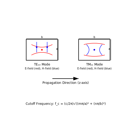
Waveguides support distinct electromagnetic field configurations known as modes, which are solutions to Maxwell's equations under the waveguide's boundary conditions. These modes are classified as transverse electric (TE), transverse magnetic (TM), or transverse electromagnetic (TEM), depending on the field components present.
TE and TM Modes
In TE modes, the electric field is entirely transverse to the direction of propagation, meaning there is no longitudinal electric field component (Ez = 0). Conversely, TM modes have no longitudinal magnetic field component (Hz = 0). The governing equations for these modes are derived from the wave equation in cylindrical or rectangular coordinates, depending on the waveguide geometry.
Here, kc is the cutoff wavenumber, determined by the waveguide dimensions. For a rectangular waveguide of width a and height b, the cutoff frequency for the TEmn or TMmn mode is:
where m and n are the mode indices representing the number of half-wavelength variations along the width and height, respectively.
TEM Mode
Unlike TE and TM modes, TEM modes have no longitudinal components for either the electric or magnetic fields. These modes are supported in transmission lines like coaxial cables but not in hollow waveguides, as they require two conductors to propagate. The absence of a cutoff frequency makes TEM modes ideal for broadband applications.
Mode Cutoff and Dispersion
Each mode has a specific cutoff frequency below which it cannot propagate. The propagation constant γ for a waveguide mode is given by:
where k = 2πf/c is the free-space wavenumber. Below cutoff, γ is purely real (β = 0), resulting in evanescent fields. Above cutoff, γ becomes purely imaginary (α = 0), allowing propagation.
Practical Implications
In real-world applications, waveguides are typically operated in the dominant mode (TE10 for rectangular waveguides), which has the lowest cutoff frequency. Higher-order modes introduce dispersion and power loss, making them undesirable for most applications. Mode suppression techniques, such as careful dimensioning and mode filters, are often employed to ensure single-mode operation.

1.3 Cutoff Frequency and Wavelength
The cutoff frequency (fc) is a fundamental property of waveguide transmission lines, defining the lowest frequency at which a given mode can propagate. Below this frequency, the mode becomes evanescent, decaying exponentially along the waveguide. The cutoff frequency is determined by the waveguide's geometry and the mode of propagation (TE, TM, or TEM).
Mathematical Derivation of Cutoff Frequency
For a rectangular waveguide with width a and height b, the cutoff frequency for TEmn or TMmn modes is derived from solving Maxwell's equations with boundary conditions. The wave equation in a waveguide leads to:
where kc is the cutoff wavenumber, and m, n are the mode indices. The cutoff frequency is then:
For the dominant TE10 mode (m=1, n=0), this simplifies to:
Cutoff Wavelength
The cutoff wavelength (λc) is the wavelength in free space corresponding to the cutoff frequency:
For the TE10 mode in a rectangular waveguide:
This means the waveguide width a must be at least half the free-space wavelength to support propagation.
Dispersion and Phase Velocity
Above the cutoff frequency, the propagation constant β is real and given by:
where k = 2\pi f \sqrt{\mu\epsilon} is the wavenumber in the unbounded medium. The phase velocity (vp) exceeds the speed of light in the medium:
This superluminal behavior is a consequence of waveguide dispersion and does not violate relativity, as information travels at the group velocity.
Practical Implications
- Waveguide Bandwidth: The usable frequency range is typically between 1.25fc and 1.89fc to avoid higher-order modes.
- Mode Suppression: Careful design ensures only the desired mode propagates, minimizing interference.
- Millimeter-Wave Applications: Waveguides are preferred at high frequencies due to lower losses compared to coaxial lines.
Historical Context
The concept of cutoff frequency was first rigorously analyzed in the 1930s during the development of radar systems. Waveguides replaced coaxial lines in microwave systems due to their lower attenuation and higher power-handling capabilities.

2. Rectangular Waveguides
Rectangular Waveguides
Fundamental Structure and Modes
Rectangular waveguides consist of a hollow metallic structure with a rectangular cross-section, typically defined by width a and height b, where a > b. The dominant mode of propagation in such waveguides is the TE10 mode, where the electric field has no component in the direction of propagation (Transverse Electric) and varies sinusoidally along the width.
The cutoff frequency for the TEmn modes in a rectangular waveguide is given by:
where c is the speed of light in free space, and m, n are the mode indices. For the TE10 mode (m=1, n=0), the cutoff frequency simplifies to:
Field Distribution and Wave Impedance
The electric and magnetic field components for the TE10 mode can be derived from Maxwell's equations. The non-zero field components are:
The wave impedance for the TE10 mode is frequency-dependent and given by:
where η is the intrinsic impedance of free space (≈377Ω) and f is the operating frequency.
Power Handling and Attenuation
The maximum power capacity of a rectangular waveguide is limited by dielectric breakdown. For air-filled waveguides, the power handling capability for the TE10 mode is:
where Emax is the breakdown electric field strength of air (≈3×10⁶ V/m).
Attenuation in rectangular waveguides arises from conductor losses and is given by:
where Rs is the surface resistance of the waveguide walls.
Practical Design Considerations
Standard rectangular waveguide dimensions are designated by WR numbers (e.g., WR-90), where the number approximates the inner width in hundredths of an inch. Key design parameters include:
- Operating bandwidth: Typically 1.25:1 to avoid higher-order modes.
- Material selection: Copper or aluminum for low-loss applications.
- Manufacturing tolerances: Critical for maintaining consistent impedance.
Waveguide flanges (e.g., UG, CPR) ensure proper impedance matching and mechanical connection between sections.
Applications in Modern Systems
Rectangular waveguides are used in:
- High-power radar systems (X-band and above)
- Satellite communication feed networks
- Particle accelerator RF cavities
- Millimeter-wave imaging systems
Recent advances include metamaterial-loaded waveguides for size reduction and dielectric-filled waveguides for flexible routing in compact systems.

2.2 Circular Waveguides
Circular waveguides are cylindrical structures that support electromagnetic wave propagation along their axial direction. Unlike rectangular waveguides, their cross-section is defined by a radius a, leading to distinct modal characteristics and cutoff conditions. The cylindrical symmetry simplifies certain analytical treatments but introduces Bessel functions into the field solutions.
Field Solutions and Modal Structure
The electric and magnetic fields in a circular waveguide are derived from Maxwell's equations in cylindrical coordinates (ρ, φ, z). For transverse-electric (TE) modes, the axial electric field is zero, while for transverse-magnetic (TM) modes, the axial magnetic field is zero. The general solution for the axial field component ψ (either Ez or Hz) is given by:
Here, Jm and Ym are Bessel functions of the first and second kind, respectively, m is the azimuthal mode number, and kc is the cutoff wavenumber. The finiteness of the field at ρ = 0 requires B = 0, simplifying the solution to:
Cutoff Conditions and Dominant Mode
The cutoff wavenumber kc is determined by boundary conditions. For TM modes, the tangential electric field must vanish at ρ = a, leading to:
The roots of this equation define the cutoff frequencies. The first non-trivial solution occurs for m = 0, yielding the TM01 mode with cutoff wavenumber kc = 2.405/a. For TE modes, the boundary condition requires:
The TE11 mode has the lowest cutoff frequency, making it the dominant mode in circular waveguides. Its cutoff wavenumber is kc = 1.841/a.
Attenuation and Power Handling
Attenuation in circular waveguides arises from conductor and dielectric losses. The attenuation constant α for TE modes is given by:
where Rs is the surface resistance, η is the intrinsic impedance, and u'mn is the n-th root of J'm(x). Circular waveguides exhibit lower attenuation than rectangular waveguides for certain modes, making them suitable for high-power and long-distance applications.
Practical Applications
Circular waveguides are employed in radar systems, satellite communications, and particle accelerators. Their rotational symmetry makes them ideal for rotating joints in radar antennas. The TE01 mode, despite not being dominant, is used in long-distance millimeter-wave transmission due to its exceptionally low attenuation.

2.3 Ridged and Flexible Waveguides
Ridged Waveguides
Ridged waveguides are a specialized variant of rectangular waveguides that incorporate one or more metallic ridges protruding into the central cavity. These ridges modify the waveguide's electromagnetic field distribution, enabling unique propagation characteristics. The primary advantage of ridged waveguides is their extended bandwidth compared to conventional rectangular waveguides. The cutoff frequency for the dominant TE10 mode is lowered, while higher-order modes are suppressed, resulting in a wider single-mode operating range.
The propagation constant γ for a ridged waveguide can be derived by solving Maxwell's equations with modified boundary conditions. For a symmetric double-ridged waveguide, the cutoff wavelength λc is approximated by:
where a and b are the waveguide's width and height, b' is the reduced height due to ridges, and s is the ridge spacing. The increased capacitance between ridges lowers the waveguide's characteristic impedance, typically ranging from 30Ω to 70Ω, compared to 50Ω in standard waveguides.
Flexible Waveguides
Flexible waveguides are essential for applications requiring mechanical adaptability, such as aerospace systems or medical equipment. These waveguides are constructed from corrugated or helical metallic structures, often plated with silver or gold to minimize resistive losses. The primary challenge in flexible waveguide design is maintaining consistent impedance and minimizing mode conversion during bending.
The bending radius R of a flexible waveguide must satisfy:
where λg is the guided wavelength, Z0 is the characteristic impedance, and ΔZ is the tolerable impedance variation. Practical flexible waveguides exhibit insertion losses of 0.1–0.5 dB/meter at microwave frequencies, with performance degrading sharply beyond critical bend radii.
Comparative Analysis
The table below summarizes key parameters for ridged versus flexible waveguides:
| Parameter | Ridged Waveguide | Flexible Waveguide |
|---|---|---|
| Bandwidth | 1.5–2× standard waveguide | Comparable to standard |
| Power Handling | 20–30% reduction | 40–60% reduction |
| Typical Applications | Wideband radar, satellite coms | Phased arrays, endoscopic devices |
Manufacturing Considerations
Modern ridged waveguides are typically machined from aluminum blocks using CNC milling, with precision tolerances of ±5μm required for optimal performance. Flexible waveguides employ electroformed nickel or copper alloys, with proprietary corrugation patterns to balance flexibility and wave guidance. Recent advances include additive manufacturing techniques for complex ridge geometries and polymer-based flexible waveguides for millimeter-wave applications.
3. Couplers and Adapters
3.1 Couplers and Adapters
Fundamentals of Waveguide Couplers
Waveguide couplers are passive devices designed to transfer electromagnetic energy between two or more waveguide structures with controlled coupling coefficients. The coupling mechanism relies on the interaction of evanescent fields or apertures that enable power division. The most common types include directional couplers, hybrid couplers, and multihole couplers, each serving distinct applications in microwave systems.
The coupling factor C (in dB) is defined as:
where P1 is the input power and P2 is the coupled power. Directivity D, a critical performance metric, quantifies the coupler's ability to isolate forward and backward waves:
Here, P3 represents the power at the coupled port for forward propagation, while P4 denotes leakage power due to backward coupling.
Types of Waveguide Couplers
Directional Couplers
Directional couplers are four-port devices with isolated ports that split signals based on propagation direction. The Bethe-hole coupler, a classic design, uses a single aperture between waveguides. Its coupling coefficient is derived from small-aperture theory:
where κ is the coupling coefficient, P0 is the incident power, and H1, H2 are the magnetic fields in the primary and secondary waveguides.
Hybrid (90° and 180°) Couplers
Hybrid couplers provide equal power division with either 90° (quadrature) or 180° (magic-T) phase shifts. The branch-line hybrid, operating at quarter-wavelength (λ/4) dimensions, exhibits the following scattering matrix for ideal operation:
Waveguide Adapters
Adapters enable impedance matching and mode conversion between dissimilar waveguide geometries or transmission media. Common types include:
- E-plane to coaxial adapters: Utilize a tapered probe to transition from TEM to TE10 modes.
- Waveguide-to-microstrip transitions: Employ finline or ridge waveguide structures to match field patterns.
- Reducing adapters: Step changes in waveguide dimensions while maintaining cutoff frequency constraints.
The voltage standing wave ratio (VSWR) of an adapter is minimized when the reflection coefficient Γ satisfies:
Optimal designs achieve VSWR < 1.2:1 across the operational bandwidth.
Practical Considerations
Manufacturing tolerances critically affect coupler performance. For a multihole directional coupler, the phase error Δφ between adjacent apertures must satisfy:
where λg is the guide wavelength and d is the inter-aperture spacing. Material selection (e.g., oxygen-free copper for low-loss applications) and surface finish (typically better than 16 μin RMS) further influence insertion loss and power handling.
In satellite communications, couplers with >30 dB directivity are employed for precise signal monitoring, while radar systems often use high-power hybrids with >1 kW handling capacity. Modern computer-aided design tools leverage finite-element method (FEM) simulations to optimize these parameters before fabrication.

3.2 Attenuators and Phase Shifters
Fundamentals of Waveguide Attenuators
Waveguide attenuators are passive devices designed to reduce signal amplitude without introducing significant phase distortion. The attenuation mechanism relies on either resistive loss or waveguide mode conversion. For rectangular waveguides operating in TE10 mode, the attenuation constant α is derived from the power dissipation per unit length:
where Rs is the surface resistance, a and b are waveguide dimensions, β is the propagation constant, and k is the wavenumber. Practical implementations use:
- Flap attenuators: Rotatable resistive cards that extend into the E-field region
- Piston attenuators: Movable lossy vane along the waveguide axis
- Fixed attenuators: Dielectric-loaded sections with controlled loss tangent
Phase Shifter Design Principles
Waveguide phase shifters modify the electrical length of the transmission path through one of three mechanisms:
where λg is the guide wavelength. Common implementations include:
Dielectric Phase Shifters
A movable dielectric slab (εr > 1) inserted into the waveguide increases the effective permittivity, reducing phase velocity. The phase shift per unit length is:
Ferrite Phase Shifters
Non-reciprocal devices exploiting the Faraday rotation effect in biased ferrite materials. The differential phase shift between forward and reverse propagation is:
where γ is the gyromagnetic ratio, Ms is saturation magnetization, and L is the interaction length.
Practical Implementation Considerations
For millimeter-wave applications (60-110 GHz), modern phase shifters achieve 0.1° resolution with insertion loss below 1 dB. Key design tradeoffs include:
- Bandwidth vs. phase resolution: Wider bandwidth designs typically sacrifice phase granularity
- Power handling: Ferrite devices handle higher power (kW range) than dielectric designs
- Temperature stability: Coefficient of phase variation typically 0.01°/°C for precision instruments
Recent advances in metamaterial-loaded waveguides demonstrate electronically tunable phase shifts up to 360° with 3:1 bandwidth ratios, enabled by varactor-diode controlled unit cells spaced at λg/4 intervals.

3.3 Terminations and Loads
Impedance Matching and Reflections
In waveguide systems, terminations are critical for minimizing reflections and ensuring maximum power transfer. When a waveguide is terminated with a load impedance ZL that differs from its characteristic impedance Z0, a reflected wave is generated. The reflection coefficient Γ quantifies this mismatch:
For perfect matching (Γ = 0), ZL must equal Z0. Mismatches lead to standing waves, characterized by the voltage standing wave ratio (VSWR):
Types of Terminations
Waveguide terminations fall into three categories:
- Matched Loads: Absorb all incident power, typically using lossy materials (e.g., carbon-loaded dielectrics) or tapered resistive films.
- Short Circuits: Reflect all power with a phase inversion (Γ = -1). Used in tuning stubs and resonant cavities.
- Reactive Loads: Introduce purely imaginary impedances (capacitive or inductive), common in filters and impedance transformers.
Practical Implementation
Matched terminations are often realized via ridged waveguide absorbers or ferrite tiles, which attenuate propagating modes without significant reflections. For example, a quarter-wave transformer can match a load to the waveguide by introducing an intermediate impedance:
This technique is widely used in radar and satellite communications to minimize return loss at the feed horn interface.
Case Study: Waveguide-to-Coaxial Transition
In hybrid systems, a common challenge is terminating a waveguide into a coaxial line. A well-designed transition uses a stepped impedance transformer to match the waveguide's TE10 mode (typically ~500 Ω) to the coaxial line's 50 Ω impedance. The transformer's length is derived from:
where λg is the guided wavelength, a is the waveguide width, and εr is the dielectric constant.
High-Power Considerations
Under high power (e.g., in particle accelerators), terminations must dissipate kilowatts of energy without arcing. Water-cooled loads or distributed lossy ceramics are employed, with careful attention to thermal expansion and mode purity.

4. Characteristic Impedance of Waveguides
4.1 Characteristic Impedance of Waveguides
The characteristic impedance (Z0) of a waveguide is a fundamental parameter that governs power transfer efficiency and impedance matching in microwave systems. Unlike transmission lines, where Z0 is purely a function of distributed capacitance and inductance, waveguides exhibit frequency-dependent impedance due to their distributed electromagnetic field structure.
Mathematical Derivation
For a rectangular waveguide operating in the dominant TE10 mode, the characteristic impedance is derived from the transverse electric and magnetic fields (Ey and Hx). Starting with Maxwell's equations in phasor form:
Solving for the field components in the waveguide yields:
where a is the waveguide width, β is the propagation constant, and ZTE is the wave impedance for TE modes:
Here, η is the intrinsic impedance of the medium (≈377Ω for air), fc is the cutoff frequency, and f is the operating frequency. The characteristic impedance Z0 is then:
where b is the waveguide height and λg is the guide wavelength.
Frequency Dependence and Practical Implications
Waveguide impedance increases with frequency, contrasting with transmission lines where Z0 is constant. This has critical design consequences:
- Impedance matching requires careful consideration of the operating frequency band.
- Power handling is maximized when the waveguide is operated well above cutoff (typically 1.25×fc).
- Dispersion effects become significant near cutoff, limiting bandwidth.
Measurement Techniques
Experimental determination of waveguide impedance employs:
- Slotted line measurements using voltage standing wave ratio (VSWR) to infer impedance.
- Time-domain reflectometry for broadband characterization.
- Network analyzers with waveguide calibration standards.

4.2 Impedance Matching Techniques
Impedance matching in waveguide transmission lines is critical to minimize reflections and maximize power transfer. Unlike transmission lines, waveguides do not have a unique characteristic impedance in the same sense as TEM lines, but matching is still essential to ensure efficient energy propagation.
Quarter-Wave Transformers
A quarter-wave transformer is a classic technique for impedance matching in waveguides. The transformer consists of a section of waveguide with a length of λg/4, where λg is the guide wavelength. The impedance of this section is chosen such that:
where Z0 is the source impedance, and ZL is the load impedance. This method is frequency-dependent and works optimally at the design frequency.
Multi-Section Transformers
For broader bandwidth matching, multi-section quarter-wave transformers are employed. By cascading multiple sections with gradually varying impedances, the reflection coefficient is minimized over a wider frequency range. The Chebyshev or binomial impedance tapering profiles are commonly used for optimal performance.
where Γn are the reflection coefficients at each discontinuity, β is the propagation constant, and l is the length of each section.
E-Plane and H-Plane Tapered Transitions
Waveguide tapers provide a gradual transition between two impedances by smoothly varying the waveguide dimensions. E-plane tapers adjust the height, while H-plane tapers adjust the width. The Klopfenstein taper is a widely used profile for minimal reflection over a broad bandwidth:
where A is a design parameter controlling the taper's performance, and L is the taper length.
Post and Iris Matching
Discontinuities such as inductive posts or capacitive irises can be strategically placed in the waveguide to cancel reflections. The equivalent circuit model for a post or iris is a shunt reactance, which can be adjusted to achieve matching:
where d is the distance from the load to the matching element.
Dielectric Slab Matching
A dielectric slab inserted into the waveguide can modify the effective impedance by altering the propagation constant. The slab's permittivity and thickness are chosen to achieve the desired impedance transformation:
where εeff is the effective permittivity of the loaded waveguide.
Practical Considerations
In real-world applications, manufacturing tolerances, material losses, and dispersion effects must be accounted for. Full-wave electromagnetic simulations (e.g., HFSS or CST) are often used to optimize matching structures before fabrication.

Reflection and Standing Waves
When an electromagnetic wave propagates through a waveguide, impedance mismatches at discontinuities or terminations cause partial or total reflection. The superposition of incident and reflected waves results in a standing wave pattern, characterized by alternating regions of maximum and minimum field intensity.
Reflection Coefficient
The reflection coefficient Γ quantifies the fraction of the incident wave reflected at an impedance discontinuity. For a waveguide with characteristic impedance Z0 terminated by load impedance ZL, the voltage reflection coefficient is:
This complex quantity encodes both magnitude and phase shift of the reflected wave. Special cases include:
- Matched load (ZL = Z0): Γ = 0 (no reflection)
- Open circuit: Γ = +1 (total reflection, in-phase)
- Short circuit: Γ = -1 (total reflection, 180° phase shift)
Standing Wave Ratio
The standing wave ratio (SWR) measures the interference pattern's contrast:
Practical implications include:
- SWR = 1 indicates perfect impedance matching
- Higher SWR values correspond to increased reflected power and potential damage to sources
- Precision waveguide systems typically maintain SWR < 1.5
Field Patterns in Rectangular Waveguides
For TE10 mode propagation, the electric field forms a standing wave pattern:
where a is the waveguide width and β the propagation constant. The resulting pattern features:
- Nulls at fixed positions where incident and reflected waves cancel
- Peaks at anti-nodes where constructive interference occurs
- Periodicity of λg/2 along the propagation axis
Power Flow Considerations
The net power transfer combines forward and reflected components:
This relationship underscores the importance of impedance matching in high-power waveguide systems, where reflected power can cause heating and reduce efficiency.
Measurement Techniques
Practical characterization methods include:
- Slotted line measurements: Mechanical probes detect field minima/maxima to determine SWR and Γ
- Vector network analyzers: Provide complex Γ measurements across frequency bands
- Time-domain reflectometry: Locates discontinuities by analyzing reflected pulse timing
Modern waveguide systems often incorporate tuners or adaptive matching networks to dynamically minimize reflections across operating conditions.

5. Microwave and RF Systems
Waveguide Transmission Lines
Fundamentals of Waveguides
Waveguides are hollow metallic structures designed to propagate electromagnetic waves at microwave and RF frequencies with minimal loss. Unlike coaxial cables, which rely on TEM (Transverse Electromagnetic) mode propagation, waveguides support TE (Transverse Electric) and TM (Transverse Magnetic) modes. The dominant mode in rectangular waveguides is TE10, characterized by its cutoff frequency:
where c is the speed of light and a is the broader dimension of the waveguide. Below this frequency, the waveguide behaves as an evanescent filter, attenuating signals exponentially.
Wave Impedance and Propagation
The wave impedance for TE and TM modes differs from the intrinsic impedance of free space (377 Ω). For TE modes, the impedance increases with frequency:
where Z0 is the free-space impedance. Conversely, TM modes exhibit a decreasing impedance trend:
These impedance variations are critical when designing impedance-matching networks for waveguide-fed antennas or filters.
Dispersion and Group Velocity
Waveguides exhibit frequency-dependent phase velocity (vp) and group velocity (vg):
This dispersion causes signal distortion in broadband applications, necessitating compensation techniques like phase equalizers in radar and satellite systems.
Practical Considerations
Waveguide selection depends on:
- Frequency range: WR-90 (8.2–12.4 GHz) is standard for X-band radar.
- Power handling: Larger cross-sections reduce ohmic losses at high power.
- Manufacturing tolerances: Dimensional errors shift cutoff frequencies and cause mode mixing.
Real-World Applications
Waveguides are indispensable in:
- Radar systems: Low-loss transmission for high-power pulses.
- Satellite communications: Millimeter-wave feeds in parabolic antennas.
- Particle accelerators: RF cavities for charged-particle acceleration.
Comparative Analysis with Transmission Lines
Key trade-offs between waveguides and TEM lines (e.g., coaxial cables):
- Advantages: Lower loss (~0.1 dB/m at 10 GHz), higher power capacity.
- Disadvantages: Bulkier, narrowband operation, higher cost.
Mathematical Derivation: Attenuation Constant
The attenuation constant (α) due to conductor losses in a rectangular waveguide (TE10 mode) is derived from Poynting vector analysis:
where Rs is the surface resistance, and a, b are waveguide dimensions. Dielectric losses add a secondary term:
with k as the wavenumber and tan δ as the loss tangent.
5.2 Radar and Satellite Communications
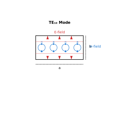
Waveguides play a critical role in high-frequency radar and satellite communication systems due to their low loss and high power-handling capabilities. Unlike coaxial cables, waveguides support propagation in the transverse electric (TE) or transverse magnetic (TM) modes, making them ideal for microwave and millimeter-wave applications.
Waveguide Propagation Modes in Radar Systems
In radar systems, waveguides are used to transmit high-power microwave signals between the transmitter and antenna. The dominant mode, TE10, is preferred due to its simple field structure and minimal dispersion. The cutoff frequency for the TE10 mode in a rectangular waveguide is given by:
where c is the speed of light and a is the broader dimension of the waveguide. For frequencies above fc, the waveguide operates with minimal attenuation, making it suitable for high-power radar pulses.
Waveguide Loss Mechanisms
Despite their advantages, waveguides exhibit losses due to:
- Conductor losses: Caused by finite conductivity of the waveguide walls, quantified by the surface resistance Rs.
- Dielectric losses: Arising from the permittivity of the medium inside the waveguide (typically air in radar applications).
- Mode conversion losses: Occur due to imperfections in waveguide geometry, leading to unwanted higher-order modes.
The total attenuation constant α for the TE10 mode can be approximated as:
where αc is the conductor attenuation and αd is the dielectric attenuation.
Waveguide Applications in Satellite Communications
In satellite communications, waveguides are used in feed networks for parabolic antennas and transponder systems. Circular waveguides (TE11 mode) are often employed due to their rotational symmetry, which simplifies alignment with the antenna feed. The waveguide’s ability to handle high power is crucial for uplink transmissions from ground stations to satellites.
The phase velocity vp and group velocity vg in a waveguide are frequency-dependent and given by:
This dispersion relationship must be accounted for in broadband satellite signals to prevent signal distortion.
Practical Considerations in Waveguide Design
For optimal performance in radar and satellite systems, waveguides must be designed with attention to:
- Impedance matching: Minimizing reflections at junctions using tapered transitions or irises.
- Power handling: Ensuring the waveguide dimensions and material can withstand high peak power without breakdown.
- Environmental sealing: Preventing moisture ingress, which can increase dielectric losses.
Advanced manufacturing techniques, such as precision milling and electroforming, are employed to achieve the tight tolerances required for high-frequency waveguide operation.

5.3 Medical and Industrial Applications
Medical Imaging and Therapy
Waveguides play a critical role in modern medical imaging systems, particularly in magnetic resonance imaging (MRI) and microwave hyperthermia therapy. In MRI systems, waveguides transmit high-frequency RF signals (typically 64–300 MHz for 1.5–7 Tesla systems) between the RF coils and the receiver electronics. The waveguide's low-loss characteristics ensure minimal signal degradation, preserving image fidelity. The cutoff frequency fc must be carefully selected to avoid higher-order modes:
where c is the speed of light and a is the waveguide's broader dimension. For a rectangular waveguide operating at 128 MHz (common in 3T MRI), a must exceed 1.17 m to ensure single-mode propagation.
In microwave hyperthermia therapy, waveguides deliver controlled electromagnetic energy to tumor tissues. The specific absorption rate (SAR) is governed by:
where σ is tissue conductivity, E is the electric field strength, and ρ is tissue density. Waveguides enable precise energy deposition by maintaining field uniformity across the applicator aperture.
Industrial Heating and Processing
Industrial microwave systems (2.45 GHz or 915 MHz ISM bands) employ waveguides for material processing applications such as:
- Plasma generation: Waveguides couple microwave energy into gas discharges for semiconductor etching and thin-film deposition.
- Food sterilization: TE10 mode waveguides ensure even energy distribution in continuous-flow pasteurization systems.
- Polymer curing: Multi-port waveguide systems provide uniform heating for composite material fabrication.
The power transfer efficiency η between a magnetron source and waveguide is given by:
where Zw is the waveguide impedance and Zs is the source impedance. Modern systems achieve >95% efficiency through quarter-wave impedance transformers.
Particle Accelerators
Waveguides form the backbone of linear accelerator (LINAC) RF structures. The shunt impedance per unit length (r) determines acceleration efficiency:
where ΔV is the voltage gain per cell and PL is the power loss. Disk-loaded waveguides optimize this parameter through periodic cavity dimensions, with typical values reaching 50 MΩ/m in medical LINACs (6–20 MeV range).
Non-Destructive Testing
Millimeter-wave waveguides (30–300 GHz) enable high-resolution material inspection. The spatial resolution δ scales with wavelength λ:
where εr is the material's relative permittivity. W-band (75–110 GHz) waveguide probes achieve sub-millimeter resolution for composite material defect detection, with sensitivity to cracks as small as 50 μm.
6. Key Textbooks and Papers
6.1 Key Textbooks and Papers
- THEORY OF WAVEGUIDES AND TRANSMISSION LINES (PDFDrive) | PDF ... — This document provides course notes on the theory of waveguides and transmission lines. It covers topics such as modes of classical transmission lines, multiport network theory using matrix descriptions, classical transmission line excitation and coupling, pulse propagation and distortion, and hollow metallic waveguides. The document contains chapters with detailed explanations, examples ...
- Microwave and RF Design - Transmission Lines, 2019a — This chapter begins with Section 6.2 where symmetries and restricting (a) Rectangular waveguide (b) Definition of planes Figure 6-1: Rectangular waveguide. 254 STEER MICROWAVE AND RF DESIGN: TRANSMISSION LINES Figure 6-2: Parallel-plate waveguide. propagation to only the ±z direction are applied to Maxwell's equations to yield the ...
- PDF Electromagnetic Waveguides and Transmission Lines — 3.7 The junction of waveguides 3.8 The connection of a waveguide to a generator 3.9 Properties of waveguide junctions 3.10 Power-based transmission line models 3.11 Anisotropic and bianisotropic waveguides 3.12 Exercises
- (PDF) Transmission lines and Waveguides notes - Academia.edu — This document discusses the concepts and mathematical foundations of transmission lines and waveguides, focusing primarily on decibels and the neper as measurement units, alongside their applications in relevant fields. It examines the properties of power and field quantities in relation to decibel calculations, outlines the characteristics of radio frequency lines such as open wire and ...
- PDF Transmission lines - api.pageplace.de — Transmission lines This rigorous treatment of transmission lines presents all the essential concepts in a clear and straightforward manner. Key principles are demonstrated by numer-ous practical worked examples and illustrations, and complex mathematics is avoided throughout.
- PDF Waveguides and Equivalent Transmission Lines — Waveguides and Equivalent Transmission Lines A waveguide is a device for transferring electromagnetic energy from one point to another without appreciable loss. In its simplest form it consists of a hollow metallic tube of rectangular or circular cross section, within which electromag-netic waves can propagate.
- 6: Waveguides - Engineering LibreTexts — Examples of such problems include analysis of the fields within microstrip line and propagation of radio waves in the ionosphere. 6.3: Parallel Plate Waveguide- TE Case, Electric Field Previously the parallel plate waveguide was introduced and we described the decomposition of the problem into its TE and TM components.
- PDF Chapter 6 Transmission Lines - University of Houston — (TEM mode) The Transverse Electromagnetic Fields in a Parallel Waveguide are approximately as follows: = E x ˆ E - jkz 0 e 6.1a
- PDF Theory of Waveguides and Transmission Lines — The e ect of this upon the distributed constant model of this transmission line is the insertion of an additional distributed capacitance into the line, in the form of an elastance2sz in series with the series inductance lz for a small length zof the transmission line.
- PDF 6 Transmission Lines - Springer — A loss-free transmission line of characteristic impedance 50 0 is terminated at one end in a short-circuit and at the other end in a resistive impedance of 85 n.
6.2 Online Resources and Tutorials
- PDF Introduction to RF Circuits — 2/3 8. Tapered Lines 5.8 5.9 Transmission Lines and Waveguides 2/5 9. Rectangular Waveguide & HFSS Tutorial 3.3 3.1-3.2 2/7 10. Modes and Propagation Behavior 3.10 2/10 11. Wall Loss in Rectangular Waveguide 2/12 12. Circular and Ridged Waveguide 3.4 2/14 13. Coaxial Cables and Microwave Connectors 3.5 2/17 14.
- Textbook contents | Electromagnetic Field Theory: A Problem Solving ... — Learning Resource Types menu_book Online Textbook. assignment_turned_in Problem Sets ... 8.1 The transmission line equations, pp. 568-579. 8.2 Transmission line transient waves, pp. 579-595 ... 8.4 Arbitrary impedance terminations, pp. 607-620. 8.5 Stub tuning, pp. 620-629. 8.6 The rectangular waveguide, pp. 629-644. 8.7 Dielectric waveguide ...
- PDF Chapter 6 Transmission Lines - University of Houston — 6-2 Popular Mechanics, 1955. 6-3 0 0 1 2 ... Parallel Plate Waveguide are approximately as follows: Using the General Definitions. 6-6 The time-average power transmitted ... Transmission Line Equations (Parallel plate waveguide) 6-16 2 2 2 +-+-0 0 wave equation V LCV 0 VV V 1 I VV Z LC L Z C-jkz jkz
- THEORY OF WAVEGUIDES AND TRANSMISSION LINES (PDFDrive) — This document provides course notes on the theory of waveguides and transmission lines. It covers topics such as modes of classical transmission lines, multiport network theory using matrix descriptions, classical transmission line excitation and coupling, pulse propagation and distortion, and hollow metallic waveguides. The document contains chapters with detailed explanations, examples ...
- PDF 7 Circuits, Transmission Lines, and Waveguides — 7.2 Wires and Transmission Lines 85 I Figure 7.3. A solenoid; the dotted line closes the integration path. Problem 6.3 showed that the energy stored in a solenoid is LI2/2. If the current flowing through an inductor is I = eiωt then the voltage drop across it is V = Liωeiωt, and so the impedance is Z = Liωeiωt eiωt = iωL . (7.25)
- PDF Transmission Lines and Waveguides - lbrce.ac.in — Types of transmission lines Waveguides 1.A transmission line consisting of a suitable shaped hallow conductor, which may be filled with a dielectric material and is used to guide EM wave of UHF propagated along its length is called a waveguide 2.Waveguide allow to pass different signals simultaneously. However different signals being
- 6.2: The Rectangular Wave Equation - Engineering LibreTexts — The LibreTexts libraries are Powered by NICE CXone Expert and are supported by the Department of Education Open Textbook Pilot Project, the UC Davis Office of the Provost, the UC Davis Library, the California State University Affordable Learning Solutions Program, and Merlot. We also acknowledge previous National Science Foundation support under grant numbers 1246120, 1525057, and 1413739.
- 6.1: Introduction - Engineering LibreTexts — All of the waveguide loss, as with the loss of most transmission systems, is resistive loss so minimizing current density minimizes loss. This chapter begins with Section 6.2 where symmetries and restricting. Figure \(\PageIndex{1}\): Rectangular waveguide. Figure \(\PageIndex{2}\): Parallel-plate waveguide.
- 6: Waveguides - Engineering LibreTexts — 6.2: Parallel Plate Waveguide- Introduction A parallel plate waveguide is a device for guiding the propagation of waves between two perfectly-conducting plates. Our primary interest in this structure is as a rudimentary model applicable to a broad range of engineering problems. ... Examples of such problems include analysis of the fields within ...
- PDF LECTURE NOTES 10 - University of Illinois Urbana-Champaign — surface of waveguide the inner surface of the waveguide is an equipotential, i.e. V constant at/on the inner surface of the wave guide. Since Laplace's equation does not allow local maxima or minima (extrema) anywhere except on the surfaces, then for a hollow waveguide, the potential V interior to the wave guide must be
6.3 Advanced Topics and Research Directions
- 6: Waveguides - Physics LibreTexts — 6.1: Phase and Group Velocity 6.2: Parallel Plate Waveguide- Introduction 6.3: Parallel Plate Waveguide- TE Case, Electric Field 6.4: Parallel Plate Waveguide- TE Case, Magnetic Field 6.5: Parallel Plate Waveguide- TM Case, Electric Field 6.6: Parallel Plate Waveguide- The TM₀ Mode 6.7: General Relationships for Unidirectional Waves
- THEORY OF WAVEGUIDES AND TRANSMISSION LINES (PDFDrive) | PDF ... — This document provides course notes on the theory of waveguides and transmission lines. It covers topics such as modes of classical transmission lines, multiport network theory using matrix descriptions, classical transmission line excitation and coupling, pulse propagation and distortion, and hollow metallic waveguides. The document contains chapters with detailed explanations, examples ...
- PDF 8 Circuits, Transmission Lines, and Waveguides — 8 Circuits, Transmission Lines, and Waveguides Electric and magnetic fields contain energy, which can propagate. These are the ingre-dients needed for communications; in this chapter we will look at how electromagnetic energy can be guided. We will start with low-frequency circuits, then progress through transmission lines to high-frequency waveguides.
- PDF Lecture: Transmission Lines and Waveguides - Fermilab — Transmission lines and waveguides are utilized to transfer electromagnetic waves carrying energy and information from a source to a receiver For an efficient transport one likes to guide the energy inside a line instead of spreading it out in space
- PDF Transmission lines — Transmission lines This rigorous treatment of transmission lines presents all the essential concepts in a clear and straightforward manner. Key principles are demonstrated by numer-ous practical worked examples and illustrations, and complex mathematics is avoided throughout.
- PDF Waveguides and Equivalent Transmission Lines — Waveguides and Equivalent Transmission Lines A waveguide is a device for transferring electromagnetic energy from one point to another without appreciable loss. In its simplest form it consists of a hollow metallic tube of rectangular or circular cross section, within which electromag-netic waves can propagate.
- Theory of Waveguides and Transmission Lines - ResearchGate — The branch is a crossed waveguide, in which through-cavities are formed in such a way that in the forward direction of the transmission the electromagnetic wave is without attenuation, and in the ...
- PDF 6.013 Electromagnetics and Applications, Course Notes — The main objectives of the text are to: 1) convey those big ideas essential to understanding the electromagnetic aspects of modern electrical and computer systems, 2) expose students to enough examples to make the big ideas tangible and erase most naiveté about dominant applications, 3) provide computational experience with Maxwell's equations sufficient to treat the basic examples, 4 ...
- PDF Hollow Waveguides 6 - Springer — The coaxial cylindrical waveguide, which is traditionally used on the transverse electromagnetic (TEM) main wave (Sect. 6.9.1) is the "oldest" transmission line. We investigate its higher order types: electric and magnetic waves.
- Waveguide sub‐wavelength structures: a review of principles and ... — His present research interest includes silicon photonics, planar waveguide circuits, and sub-wavelength structures. He was one of the scientists that helped start Optenia Inc. and developed the first commercial echelle grating wavelength division multiplexer.