Applied Function Generators
1. Definition and Purpose
1.1 Definition and Purpose
Applied function generators, commonly referred to as function generators, are versatile electronic testing devices that produce a wide range of electrical waveforms. These devices are fundamental in the fields of electronics and telecommunications, serving multiple purposes, from testing the frequency response of circuits to developing complex signal patterns for research and development. Understanding the definition and application of function generators is pivotal for engineers and researchers who work with electronic signal testing and manipulation.
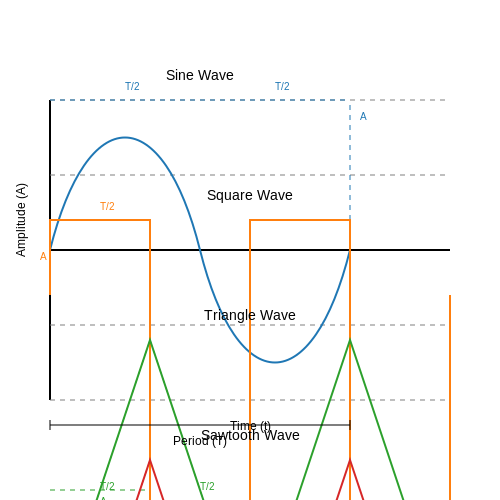
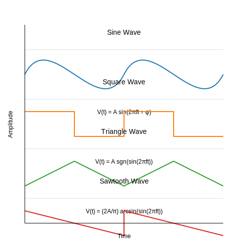
Function generators can create various types of waveforms such as sine, square, triangle, and sawtooth waves, each characterized by distinct mathematical properties and harmonic content. The ability to switch between these waveforms allows for the simulation of different conditions encountered in real-world scenarios. For instance, a sine wave can simulate an alternating current (AC) signal, while a square wave can imitate the switching behavior of digital signals.
Operational Principles
At the core of a function generator lies an oscillator circuit that defines the frequency and shape of the output waveform. Most modern function generators utilize digital synthesis techniques that provide enhanced stability and precision. The fundamental operation involves modulating parameters such as frequency, amplitude, and offset to produce the desired waveform.
A typical function generator may use a microcontroller or an analog circuit to achieve waveform generation. For example, in a digital function generator, the principle of phase-locked loops (PLLs) or direct digital synthesis (DDS) enables precise control over frequency and phase, resulting in waveform generation that is both reliable and reproducible.
Mathematical Modeling
To mathematically model a simple waveform, we can look at the sine wave, which is defined by the equation:
Here, A represents the amplitude of the wave, f is the frequency in hertz, t is time in seconds, and φ is the phase shift in radians. By varying these parameters, one can generate tailored waveforms for specific applications.
Practical Applications
The applications of function generators are vast and varied. In research laboratories, function generators are utilized to:
- Test Circuit Responses: Function generators allow engineers to input specific waveforms into circuits and observe their behavior, thus enabling troubleshooting and design validation.
- Signal Processing: They are essential in testing analog filters and amplifiers by providing signals for evaluation of frequency-domain characteristics.
- Simulation of Real-World Signals: Using varied waveforms, function generators can simulate noise, transient signals, and other distortions in electronic systems.
- Educational Purposes: In academic settings, they serve as a crucial tool for teaching concepts related to waveforms, oscillations, and signal processing.
In industrial settings, function generators play a key role in quality assurance, aiding in production testing to ensure that electronic components meet specified performance criteria. Furthermore, they have applications across various fields, including automotive, aerospace, and biomedical engineering, where testing and analysis of electronic systems are critical.
In conclusion, function generators serve as an essential tool in both theoretical and practical aspects of electronics. Their ability to generate precise and controllable waveforms makes them invaluable for a wide range of applications that require accurate signal generation. As technology evolves, advancements in function generator design continue to expand their capabilities, further enhancing their relevance in modern electronics.
1.2 Types of Function Generators
In the realm of advanced electronics, function generators are indispensable tools employed extensively in both research and industry. They serve as multifunctional signal sources that can emulate various waveforms, providing engineers and scientists with the means to generate specific electrical signals required for testing, analysis, and experimentation. Understanding the various types of function generators available can significantly influence their application in different scenarios. There are primarily three categories of function generators that distinctly define their structure and capabilities: analog function generators, digital function generators, and arbitrary waveform generators (AWGs). Each type has unique characteristics and advantages, contributing to their utilization in assorted applications.Analog Function Generators
Analog function generators are typically the most classical type, relying on analog circuitry to produce waveforms such as sine, square, and triangular waves. These generators operate by manipulating voltage-controlled oscillators (VCOs) to create a continuous range of frequencies. The tuning is done through potentiometers or variable capacitors, which can introduce certain nonlinearities into the generated waveforms. Their primary advantage lies in their simplicity and reliability for basic waveform generation. However, they are limited in frequency range and waveform fidelity, particularly at higher frequencies. This limitation is a crucial consideration in applications requiring precise signal characteristics, such as in communications or high-frequency circuit testing.Digital Function Generators
Transitioning from analog designs, digital function generators have gained popularity due to their versatility and accuracy. Utilizing digital signal processing (DSP) techniques, these generators convert mathematical functions into digital representations before producing signals. The key advantage of digital function generators is their ability to easily manipulate and store complex waveforms. Digital function generators offer enhanced stability and a broader frequency range compared to their analog counterparts. They can produce a wide array of waveforms with high precision, often allowing users to program custom sequences through software interfaces. This aspect makes them an invaluable resource in more sophisticated experiments and testing environments, such as in digital communications, audio/video processing, and embedded system development.Arbitrary Waveform Generators (AWGs)
Taking functionality to the next level, arbitrary waveform generators are specialized types of digital function generators capable of producing virtually any waveform shape defined by the user. They leverage high-resolution digital-to-analog converters (DACs) to construct waveforms based on mathematical descriptions or waveform samples. AWGs find applications beyond standard waveform generation, being particularly useful in testing and simulating real-world signals encountered in various technologies, such as telecommunications and medical devices. Their ability to replicate complex signals like pulse trains or transient responses is crucial for testing equipment against hard-to-simulate conditions. As technology evolves, the convergence between these types of function generators is notable as hybrid models emerge, combining the strengths of analog and digital methodologies to produce high-fidelity signals while maintaining user-friendly interfaces. In sum, selecting the appropriate type of function generator involves careful consideration of the application's specific requirements, including waveform fidelity, frequency range, and output capabilities. Understanding these distinctions equips researchers and engineers with the knowledge necessary to leverage function generators effectively in their work.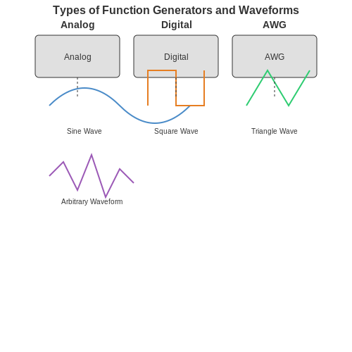
1.3 Applications in Electronics
Applied function generators are pivotal in various electronic applications, serving as essential tools for engineers, physicists, and researchers. Their capability to produce different waveform outputs—such as sine, square, triangular, and arbitrary waveforms—enables a broad range of functionalities, ranging from testing and measurement to complex signal processing.
Signal Testing and Characterization
In testing and characterizing electronic circuits, function generators provide reliable waveforms that simulate real operational conditions. For instance, when evaluating the frequency response of an amplifier circuit, a sine wave generated at varying frequencies can be injected into the input. By analyzing the output across frequency ranges, researchers can derive properties like gain and phase shift.
Moreover, function generators allow for testing under controlled conditions, ensuring that the insights gained are reproducible and reliable. This is crucial in fields such as telecommunications, where understanding signal integrity and distortion is essential for system performance.
Research and Development
In research environments, function generators play a significant role in the development of new electronic devices. They allow for precise control of signal characteristics, enabling the exploration of new circuit designs and the testing of their responses under varying conditions. For example, in analog circuit design, a triangular wave may be used to test integrators or differentiators, allowing engineers to validate their designs against expected theoretical behaviors.
Modulation Techniques
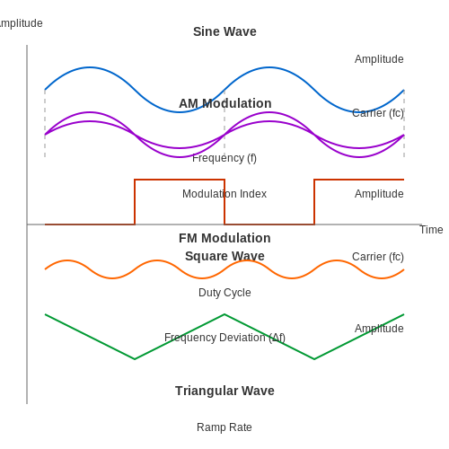
Another crucial application of function generators is in modulation techniques. They can create modulated waveforms such as amplitude modulation (AM) and frequency modulation (FM). This is particularly relevant in communication systems, where the generated modulated signals can be used for modulation of carriers prior to transmission, facilitating the study of signal processing techniques and channel behaviors.
Example: AM and FM Signal Generation
For generating an amplitude-modulated signal, the process can be described mathematically as:
Here, \( A \) represents the carrier amplitude, \( m(t) \) is the message signal, and \( f_c \) is the carrier frequency. By using a function generator to implement this equation, engineers can create a test signal that mimics real AM signals, which could be analyzed further in a lab setting.
Similarly, for frequency modulation, the signal can be represented as:
where \( k_f \) is the frequency sensitivity. Understanding these frequencies is crucial for testing modulated systems and ensuring they perform as expected.
Control Systems
Function generators also have significant implications in control systems. They can generate reference signals that simulate desired inputs for control algorithms. For instance, in examining the response of a PID controller, stepped or ramp inputs can be generated to analyze how well the controller follows the intended trajectory. This is crucial in optimizing the controller's parameters to achieve stable performance.
The adaptability of function generators makes them integral tools in educational laboratories as well as professional environments, enabling hands-on experiments that deepen the understanding of theoretical concepts.
To sum up, the applications of function generators in electronics span across testing and validation in research, exploring modulation techniques in communication systems, and enhancing control system analysis, thereby offering indispensable support in both theoretical studies and real-world applications.
2. Frequency Range
2.1 Frequency Range
In the realm of applied electronics, the concept of frequency range holds paramount importance, particularly when utilizing function generators. A function generator, as a versatile tool, synthesizes various waveforms, each defined by specific frequency ranges determined by the operating principles and architecture of the device. Understanding how these frequencies influence signal characteristics and practical applications can significantly enhance the efficacy of experimental designs.
The frequency spectrum of a function generator typically spans from ultra-low frequencies (ULF) at a few microhertz (µHz) to high frequencies (HF) reaching several megahertz (MHz) or even gigahertz (GHz) in advanced models. This wide spectrum allows for diverse applications across different fields, from characterization of electronic components to the testing of communication systems.
Key Frequency Ranges
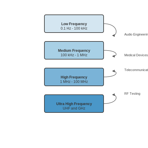
Function generators categorize their output into distinct frequency ranges, each suitable for specific applications. The low-frequency range (typically 0.1 Hz to 100 kHz) is essential for testing audio and analog circuits, as well as simulating control systems.
- Low Frequency (0.1 Hz - 100 kHz): Primarily useful in audio applications, signal processing, and testing functionality in components like resistors, capacitors, and transistors.
- Medium Frequency (100 kHz - 1 MHz): Used in RF and other high-precision applications, this range facilitates the investigation of intermediate frequency amplifiers and mixers.
- High Frequency (1 MHz - 100 MHz): Critical for generating signals used in RF circuit designs, modulation schemes, and high-speed data transmission.
- Ultra High Frequency (UHF) and GHz range: Advanced function generators are capable of generating signals useful in microwave applications, such as radar and satellite communications.
Understanding Frequency Range Limitations
Each function generator comes equipped with a maximum frequency output limit. Factors influencing this upper limit include:
- Design Architecture: Analog function generators may exhibit lower frequency limits compared to their digital counterparts, which leverage digital signal processing to achieve higher frequencies.
- Output Impedance: The impedance matching between the generator and the load affects signal integrity and frequency response, hence influencing practical use cases.
- Amplitude Modulation: Maximum amplitude and waveform fidelity may deteriorate at higher frequencies, necessitating careful consideration during signal generation.
Applications in Real-world Scenarios
The applicability of various frequency ranges extends across multiple domains:
- Audio Engineering: Testing loudspeakers and audio circuits within the low-frequency domain.
- Telecommunications: Generating RF signals for communication system testing.
- Medical Devices: Testing electrocardiograms (ECGs) within specific signal ranges to ensure operational readiness.
In summary, comprehending the frequency range capabilities of function generators serves as a cornerstone for effectively harnessing their potential in applied physics and electronics. As technology progresses, advancements in both hardware and software will further expand the frequency capabilities, pushing the boundaries of what is feasible in research and practical applications.
2.2 Waveform Types
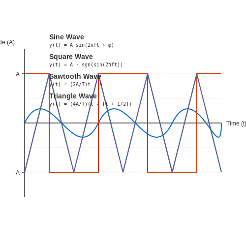
In the realm of applied function generators, understanding various waveform types is crucial for effective design and application. These waveforms serve as the backbone of countless electronic systems, each with unique characteristics that cater to specific needs in electronics and signal processing. This section delves into the primary waveform types commonly generated by function generators, examining their mathematical representations, practical relevance, and real-world applications.Sine Wave
The sine wave is the most fundamental waveform, representing an oscillation characterized by a smooth periodic rise and fall. Mathematically, it can be expressed as:- A is the amplitude, indicating the peak value of the waveform.
- f is the frequency, representing how many cycles occur per second.
- t is time.
- \(\phi\) is the phase shift, determining the horizontal displacement.
Square Wave
Square waves alternate between two levels, typically high and low, representing a binary state. The mathematical representation of a square wave can be given through its duty cycle and frequency:Sawtooth Wave
The sawtooth wave transitions linearly from its minimum to maximum value before abruptly jumping back to the minimum level, creating a distinctive ramp-up and drop-off. The mathematical form of a sawtooth waveform is:- T is the period of the wave.
- A remains the amplitude.
Triangle Wave
A triangle wave shares characteristics with both the sawtooth and square waves but has linear rise and fall segments, leading to a more gentle oscillation. Its mathematical representation is:Implications for Real-World Applications
Different waveform types play critical roles across numerous applications regardless of whether they are used in complex signal modulation techniques or simple signal testing. For instance:- In audio synthesis, composers utilize various waveforms to create unique sound textures.
- In telecommunications, modulating signals can improve data transmission rates.
- In control systems, waveform generation is vital for establishing system stability and performance.
2.3 Signal Amplitude and Offset
The concepts of signal amplitude and offset are fundamental when working with applied function generators. Understanding these parameters enables engineers and researchers to accurately characterize the output of waveforms for various applications, from audio engineering to communications.
Signal Amplitude
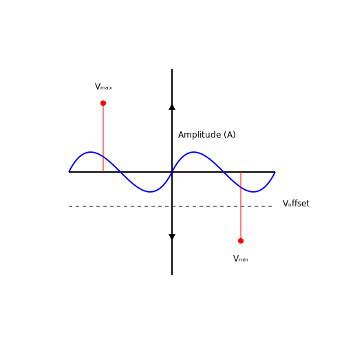
Signal amplitude refers to the maximum extent of a periodic wave, which is often measured as the voltage or current deviation from its mean value. In practical applications, amplitude can dictate how effectively a signal can drive a load or be transmitted through media.
In a sinusoidal waveform, for instance, the amplitude \( A \) can be mathematically defined by the peak-to-peak value, or the maximum displacement from the rest position.
Here, \( V_{\text{max}} \) and \( V_{\text{min}} \) represent the maximum and minimum voltages of the signal, respectively. Understanding this relationship is crucial for ensuring that output signals meet system requirements without distortion or clipping.
Signal Offset
Signal offset refers to a constant DC voltage added to an AC signal, shifting the entire waveform vertically on the voltage scale. This is especially significant in applications where direct coupling is insufficient to prevent distortion or clipping caused by the limitations of voltage thresholds in circuits.
The relationship between the input and the adjusted signal can be expressed mathematically as:
Where \( V_{\text{offset}} \) is the DC component added to the original signal \( V_{\text{input}}(t) \). Practically, offsetting signals allows for better interfacing with other electronic components that may have specific voltage requirements.
Practical Applications
Signal amplitude and offset are crucial both in the laboratory and in industrial applications. For instance, in audio synthesis, having a correct amplitude ensures the audio is audible without distortion. In communications, properly offset signals can aid in effective modulations, ensuring that data is accurately demodulated at the receiver end.
In conclusion, mastery of signal amplitude and offset empowers engineers to design robust systems that function accurately in diverse environments. As we delve further into function generators, these foundational concepts will continuously enhance your practical understanding and programming of complex waveforms.
2.4 Rise and Fall Time
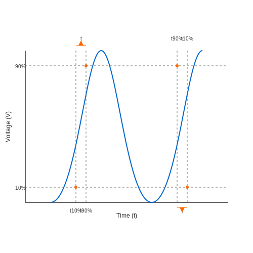
Understanding rise and fall time is critical in the application of function generators, as these parameters significantly influence both the performance and the fidelity of signal outputs in various electronic devices. Rise time refers to the time taken for a signal to change from a defined low level to a defined high level, while fall time is the opposite, evaluating how quickly a signal can drop from high to low. Both are essential metrics that affect signal integrity, switching speeds, and overall system performance.
To comprehend rise and fall times fully, we begin with the definitions. Rise time (tr) and fall time (tf) can be expressed mathematically in the context of a step response of a linear system. Typically, these values are defined as the time taken for the signal to move from 10% to 90% of its final value. This definition can be mathematically represented as:
In these equations, t90% represents the time at which the signal reaches 90% of its final amplitude, while t10% indicates the time at which the signal first reaches 10% of its final amplitude. This metric is crucial in digital circuits where rapid signaling is necessary to reduce latency and improve throughput.
To give a practical context, let us consider an operational amplifier (op-amp) configured as a comparator. In high-speed applications such as data converters, it is essential to minimize rise and fall times to ensure that the output correctly follows the fast-changing input signal. If an op-amp has a rise time of 10 microseconds, it would limit the maximum frequency it can handle without distortion to approximately 35 kHz, calculated using the relationship:
This relationship is indicative of bandwidth limitations that can be crucial in applications such as signal conditioning, communications, and pulse width modulation.
Applications and Importance
In real-world scenarios, rise and fall times play significant roles in various applications:
- Digital Signal Processing (DSP): Systems that require precise timing and synchronization must adhere to strict rise and fall time specifications to prevent timing errors.
- Telecommunications: In data transmission, longer rise and fall times can lead to increased signal degradation and bit errors, limiting data throughput.
- Control Systems: For feedback and control applications, minimizing rise and fall times enhances system responsiveness, ensuring quick adjustments to dynamic changes.
Understanding how to manage and optimize rise and fall times is critical for engineers and researchers working with high-speed circuits and systems. Advanced techniques, such as the use of buffer amplifiers or controlled rise and fall times through circuit design, can be employed to tailor the behavior of output signals, making them suitable for varying applications.
Further, rise and fall times can be affected by parasitic capacitance and inductance in circuit design, which necessitates careful layout considerations. Engineers can leverage simulation tools to predict and analyze those effects before physical prototyping, ensuring optimal performance in practice.
In conclusion, rise and fall time measurements are vital for determining the effectiveness and reliability of signal behavior in function generators. A precise understanding of these parameters enables engineers to refine circuit designs and improve overall system performance.
3. Sine Waves
3.1 Sine Waves
Sine waves are fundamental to the study and application of signals in both physics and engineering. They represent a pure frequency signal, characterized by their smooth periodic oscillations that can be described mathematically by the sine function. This section delves into the generation, properties, and applications of sine waves, highlighting their critical role in a variety of technological fronts, including telecommunications, audio engineering, and signal processing.Understanding Sine Waves
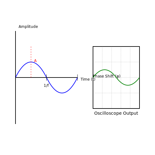
A sine wave can be described mathematically as:Practical Generation of Sine Waves
In electronics, sine waves are generated using function generators, which can create a variety of signal shapes, including sine, square, triangular, and sawtooth waves. These devices utilize various methods to produce sine waves, including:- Direct Synthesis: This method involves using digital-to-analog converters (DACs) to produce sine waves by converting digital data directly into analog signals. It's precise and highly programmable.
- Phase-Locked Loop (PLL): PLLs can produce sine waves by locking on to a reference frequency and generating an output frequency that is a multiple (or sub-multiple) of that reference frequency.
Example: Using a Function Generator
A typical function generator can be configured to produce sine waves by setting specific parameters like amplitude and frequency. The output will often be displayed on an oscilloscope, which provides a visual representation of these oscillations, making it easier to study their properties. To visualize this, imagine looking at an oscilloscope screen where a smooth wave oscillates between a defined maximum and minimum voltage level, indicative of its amplitude. The frequency determines how fast these oscillations occur; a higher frequency results in more wave cycles visible in the same time frame.Applications of Sine Waves
Sine waves have numerous applications across different fields:- Telecommunications: Sine waves are the basis for modulating signals, essential for data transmission over various media, including radio waves and fiber optics.
- Audio Engineering: In sound production, sine waves are used to synthesize tones. They represent the simplest sound waves, serving as building blocks for more complex musical notes when combined.
- Signal Processing: Sine waves play a critical role in Fourier analysis, allowing complex signals to be decomposed into their fundamental harmonic components.
3.2 Square Waves
In the realm of applied function generators, the square wave is one of the most fundamental waveforms. This subsection delves into the nature of square waves, their mathematical representation, generation techniques, and their multifaceted applications across different fields such as communications, signal processing, and electronic testing.
Understanding Square Waves
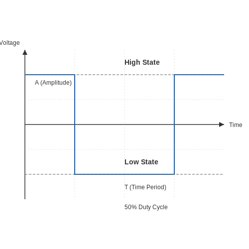
A square wave is a non-sinusoidal waveform typically characterized by its distinct rectangular shape, where the signal alternates between two levels with a defined frequency. Its value remains constant for half the period before switching to the alternate value, effectively creating a signal that is on for 50% of the time and off for the remaining half, usually visualized as a square shape when plotted over time.
The mathematical representation of a square wave can be articulated through its Fourier series. The importance of this representation lies in its ability to break down the waveform into a sum of sinusoidal functions of different frequencies:
Here, \( A \) represents the amplitude, \( f_0 \) is the fundamental frequency, and \( T \) is the time period of the square wave. The series encompasses only odd harmonics, reflecting the square wave’s rich harmonic content, which makes it especially valuable in various applications.
Generating Square Waves
When it comes to generating square waves, there are several methods employed in practice. The most common techniques include:
- Digital Circuits: Using flip-flops to create a divide-by-two circuit can produce a square wave. A basic arrangement in which a clock cycle is fed into a flip-flop can yield an output that toggles every clock pulse.
- Operational Amplifiers: By configuring an operational amplifier in an astable multivibrator mode, it’s possible to generate a square wave output. This configuration involves feedback components to establish the desired frequency.
- Function Generators: Dedicated function generation equipment can generate precise square waves with adjustable frequency and amplitude. These devices typically feature additional functionalities for varying waveform shapes and pulse duty cycles.
Applications of Square Waves
The versatility of square waves translates into numerous practical applications:
- Testing Electronic Devices: Square waves are routinely used in electronic test equipment to analyze the frequency response and characteristics of devices under test.
- Communication Systems: In digital modulation techniques, square waves are integral as they effectively represent binary data, allowing efficient information transmission.
- Clock Signals: In digital circuits, square waves serve as clock signals, synchronizing operations of the various components in digital systems.
- Signal Processing: Due to their sharp transitions, square waves can be utilized to test filters and other signal processing systems, revealing their behaviors in response to abrupt changes.
The harsh transitions inherent to square waves also provide insight into the bandwidth and frequency response characteristics of different filters, thereby making them indispensable in both laboratory conditions and in-field applications.
Ultimately, square waves exemplify the intersection of theory and practical application, making them a staple in electronics and signal processing. Their fundamental nature supports a broad spectrum of activities, ranging from straightforward signal generation to complex modulation schemes in advanced communication systems.
3.3 Triangle Waves
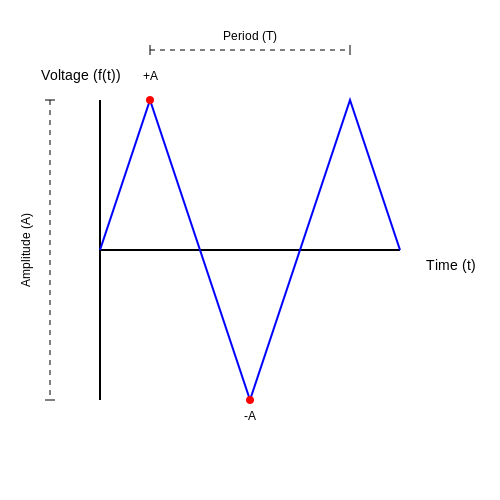
Triangle waves are fundamental waveforms in the field of electronics and signal processing, characterized by their linear rise and fall. Unlike sine waves, which exhibit smooth periodic oscillations, triangle waves have a distinctive zig-zag pattern, making them valuable in various applications, including modulation, waveform generation, and functional testing.
The mathematical representation of a triangle wave can be derived from a sawtooth wave, which is another common waveform. The triangle wave can be expressed as a function of time, defined over a period \( T \). The basic principles of triangular wave generation involve the linear ramping-up and ramping-down of voltage levels, resulting in distinct slopes during these intervals.
Mathematical Derivation
The triangle wave can be represented mathematically using the following equation:
Where:
- f(t): The output voltage at time \( t \).
- A: The amplitude of the wave.
- T: The period of the wave.
- \(\lfloor x \rfloor:\ The floor function, which returns the greatest integer less than or equal to \( x \).
Analyzing the components of the equation, we observe that the function is linear within each half of its period, increasing from -A to A in the first half and decreasing back to -A in the second half. The waveform alternates every period, displaying a consistent cycle.
Square and Periodicity
The periodic nature of triangle waves offers advantages in real-world applications, particularly in the realm of analog circuit testing and synthesis. When generating signals using function generators, triangle waves are essential for simulating various conditions when interfacing with linear systems, such as in control systems and audio applications.
Applications
Triangle waves have a range of real-world applications including:
- Signal Processing: Used in phase-locked loops (PLLs) to help synchronize signal phases.
- Modulation: Employed in frequency modulation (FM) systems.
- Audio Synthesis: Common in synthesizers to generate tones alongside other waveforms.
- Function Generators: Used in laboratories for testing electronic circuits and components.
In summary, triangle waves, inherent in nature due to their symmetry and periodicity, are critical in electronics and signal processing. Understanding their generation and dynamics is crucial for engineers and researchers engaged in developing innovative solutions across multiple domains.
3.4 Arbitrary Waveforms
Arbitrary waveforms are essential in the realm of function generators, enabling the synthesis of complex signal shapes that are not limited to basic sinusoidal, triangular, or square waves. This flexibility allows engineers and researchers to test and develop various systems under conditions that closely mimic real-world signals.
To better understand arbitrary waveforms, we will explore their definition, generation methods, practical applications, and the underlying mathematical concepts that make this functionality possible.
Understanding Arbitrary Waveforms
An arbitrary waveform can be described as a waveform that does not adhere to a standard, pre-defined shape. Instead, it can be constructed from any combination of periodic and non-periodic signals. The mathematical representation of a waveform is typically expressed as a function of time, f(t), and may include multiple frequency components. This capability is crucial for simulating real-world signals in testing environments, particularly in communication, audio, and biomedical applications.
Mathematical Representation
To generate an arbitrary waveform, we must first represent it mathematically. Consider a waveform expressed as a sum of sinusoidal components, known as a Fourier series expansion:
In this equation:
- $$a_0$$ is the average value of the function over one period.
- $$a_n$$ and $$b_n$$ are the Fourier coefficients representing the weights of the cosine and sine components, respectively.
- $$\omega_0$$ is the fundamental angular frequency of the waveform.
The ability to create complex waveforms through this method significantly enhances design testing. For practical applications, function generators often utilize digital-to-analog converters (DACs) to synthesize arbitrary waveforms from discrete samples of a continuous-time signal.
Waveform Generation Techniques
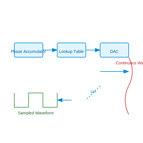
Arbitrary waveforms are typically generated using two primary techniques: Direct Digital Synthesis (DDS) and Sample-and-Hold (S/H) methods.
Direct Digital Synthesis (DDS)
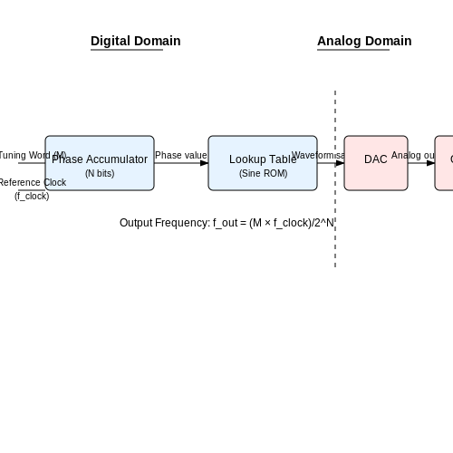
In DDS, digital signals are produced by creating discrete points of the waveform and then using a DAC to convert these digital values into analog signals. This method allows for high precision and frequency stability. The basic components of DDS include:
- Phase accumulator: Keeps a running total of phase increments based on the desired frequency.
- Waveform Look-up Table (LUT): A memory unit storing pre-calculated values of the waveform.
- DAC: Converts digital values to an analog signal.
Sample-and-Hold (S/H)
Sample-and-Hold operates by taking a sampled version of a continuous waveform at discrete intervals and holding these values steady during each interval. While not providing the same detail as DDS, it is often utilized in situations where history and accuracy are less critical.
Applications of Arbitrary Waveforms
The practical applications of arbitrary waveforms are extensive and varied. Some notable areas include:
- Testing Communication Systems: Simulating various signal types and noise conditions helps in evaluating the performance of receivers and other components.
- Audio Signal Processing: Generating customized audio waveforms for testing amplifiers, speakers, and other audio equipment.
- Biomedical Engineering: Creating specific waveforms to stimulate biological tissues or simulate physiological signals for medical equipment testing.
In conclusion, arbitrary waveforms expand the functional capabilities of function generators, enabling precision testing and research in various engineering domains. By understanding the mathematical underpinnings and generation techniques, advanced users can fully utilize these tools to effectively simulate a vast array of signals for their specific applications.
4. User Interface Overview
4.1 User Interface Overview
The user interface (UI) of a function generator is a critical component that defines the ease and efficiency with which users interact with the instrument. Understanding the elements of the interface not only aids in operation but also enhances exploration of the device's capabilities in practical scenarios. This section delves into the key components and functionalities that characterize the user interface of modern applied function generators, drawing on both technological advancements and user experiences.Key Components of the User Interface
Typically, the UI of a function generator is designed to be intuitive, comprising several key components:- Display Screen: This is a central feature that provides real-time visual feedback on waveforms, settings, and operational status. High-resolution LCDs are now common, often with touch capabilities that allow for direct manipulation of parameters.
- Control Knobs and Buttons: These allow for precise adjustments of parameters such as frequency, amplitude, and offset. Many models now feature rotary encoders that enable finer control over settings and often provide tactile feedback.
- Waveform Selection: Users can typically choose from several preset waveforms, such as Sine, Square, Triangle, and Sawtooth, often through a simple menu system or dedicated buttons.
- Output Connectors: These provide the means to connect the function generator to external circuits or equipment, and may include BNC connectors, SMA connectors, or other specialized interfaces.
- Memory Functions: Advanced models come equipped with memory slots for saving custom waveforms and settings, facilitating quick recall during experiments.
Navigating the Interface
An important aspect of the user experience is the layout and navigation of the interface. A well-structured layout typically consists of:- Main Menu: This serves as the entry point, providing access to various settings and functions, often grouped logically for ease of use.
- Submenus: Detailed settings related to waveform parameters, modulation options, and output configuration are commonly found in submenus that can be reached through the main menu.
- Status Indicators: Visual cues such as LED indicators or screen alerts inform users about the operational state, ensuring quick assessment at a glance.
Real-World Applications
Function generators play crucial roles across a range of fields including electronics testing, telecommunications, and research laboratories. For engineers and researchers, the ability to modulate waveforms and frequencies precisely is essential for simulating real-world signals in testing circuits. For instance, in telecommunications, function generators are used to simulate different types of signals to validate receiver performance. In educational settings, they serve as valuable teaching tools, allowing students to visualize and understand various waveform properties and their impact on circuit behavior. Thus, an effective user interface not only elevates operational efficiency but also fosters a more profound engagement with the science of waveforms. Overall, a well-designed user interface in function generators significantly enhances usability, contributes to accurate signal generation, and exemplifies technological advancements in instrumentation tailored for diverse applications. Understanding these components and their functionalities is essential for maximizing the potential of applied function generators.4.2 Setting Up a Function Generator
Function generators are invaluable tools in the realms of electronics and scientific research, allowing users to create waveforms of specified frequency, amplitude, and shape. Understanding how to set them up effectively is crucial for obtaining valid and meaningful results in experimental setups and design validations.
Connecting the Function Generator
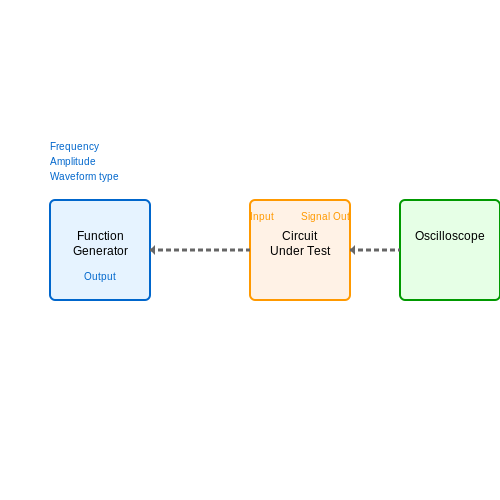
Before diving into generating signals, it's essential to correctly connect the function generator to the circuit in question. Begin by identifying the appropriate output terminals on the generator, which will typically be labeled as "Output" or "Signal Out." Most modern function generators include BNC connectors for output, which are widely used in laboratories.
Once identified, use a good quality shielded coaxial cable to connect the output of the function generator to the input of the circuit under test (CUT). This minimizes signal interference and ensures the integrity of the waveform. For practical applications, be sure to consider the load impedance of the device being tested. For instance, typical function generators are designed to drive a load of 50 ohms or high impedance inputs. Adjusting for the impedance ensures maximal power transfer according to the maximum power transfer theorem.
Powering and Configuring the Generator
After securely connecting your generator, power it on. The initial display should present you with the main configuration screen, typically showing default settings such as a sine wave at 1 kHz. Familiarize yourself with the adjustable parameters:
- Frequency: The rate at which the waveform repeats. This can usually range from microhertz to megahertz.
- Amplitude: The height of the waveform, typically expressed in volts peak-to-peak (Vpp).
- Waveform type: Common shapes include sine, square, triangle, and sawtooth.
Adjust each parameter based on your experimental needs. For example, if you are testing a low-pass filter, begin by setting the output to a sine wave at a frequency just below the expected cutoff frequency.
Output Observations and Adjustments
After configuring your desired parameters, you should observe the waveform on an oscilloscope connected to the output of the CUT. This step is essential for validating the waveform integrity. Monitor aspects such as:
- Shape: Ensure the waveform corresponds to your settings.
- Frequency: Verify that the oscilloscope's measured frequency closely matches the generator setting.
- Amplitude: Confirm that the output signal displays the intended peak-to-peak voltage.
If discrepancies arise, adjustments may be necessary. Check for the following:
- Confirm that connections are secure and free of corrosion.
- Review the input impedance of the CUT. Mismatched impedance can distort the waveform.
- Examine the oscilloscope settings for accuracy, ensuring time base and voltage scale are correctly configured.
Practical Applications
In real-world scenarios, function generators are used in various applications, including:
- Testing audio equipment with signal waves to evaluate frequency response.
- Simulating control signals in embedded systems to diagnose circuit behavior.
- Calibrating sensors and measuring devices to ensure accuracy in outputs.
Understanding how to set up a function generator effectively not only enhances the efficiency of circuit design and testing but also improves one's ability to troubleshoot and innovate within the engineering field. As your proficiency grows, consider exploring the advanced functions of your generator, such as modulations and controlled pulse generation, to expand its utility further.
4.3 Output Connections and Impedance
The output connections of a function generator, along with the characteristics of the load impedance, play a critical role in the successful application of generated signals in real-world scenarios. A solid understanding of these concepts is not only important for ensuring signal integrity but also for avoiding potential damage to both the generator and the connected devices.Understanding Output Connections
A function generator usually provides various output connections to facilitate easy integration into different circuits. These outputs can be classified based on their voltage levels (such as low-level or high-level) and format (single-ended or differential). The arrangement of these connections is critical as it influences how the signal propagates through the circuit. In applications such as circuit testing, a typical output configuration might include a banana jack, BNC connector, or even a terminal block. Each of these formats has its own set of attributes and can contribute unique challenges such as stray capacitance, poor connections, or high-frequency losses.Impedance and Its Importance
Another vital aspect that directly affects the interaction between a function generator and the load is impedance. Impedance, denoted as \( Z \), is a complex quantity that encompasses both resistance \( R \) and reactance \( X \). It is essential to understand that the function generator's output impedance is typically characterized by a low impedance (often around 50 ohms) to maintain signal integrity and minimize reflections. On the other hand, the input impedance of the load must be considered to ensure proper signal transfer. A fundamental concept in circuit design is the idea of matched impedance. When the output impedance of the generator matches the input impedance of the load, maximum power transfer occurs. In practical terms, this is expressed by the Maximum Power Transfer Theorem, which states that maximum power will be delivered to the load when: $$ Z_{\text{load}} = Z_{\text{source}} $$ where \( Z_{\text{load}} \) is the impedance of the load and \( Z_{\text{source}} \) is the output impedance of the source (the function generator). If the impedances do not match, part of the signal can be reflected back towards the generator, which may lead to distortions in the output waveform. To illustrate this concept, consider the following simple scenario in a circuit where a function generator is used to drive a resistive load:Implications of Impedance Mismatch
When an impedance mismatch occurs, the magnitude and phase of the output signal can be significantly altered. In particular: - Voltage Reflection: This phenomenon leads to partial retaining of the voltage at the source leading to less output voltage at the load. - Power Loss: Reflected signals can result in losses which may reduce the overall efficiency of the system. To visualize the impact of these principles, imagine a circuit carrying a sinusoidal signal generated by a function generator connected to a load. If both the impedance values are mismatched, this could manifest as a significant drop in voltage across the load terminals.Practical Applications and Considerations
Understanding output connections and impedance characteristics is crucial in multiple fields, including telecommunications, signal processing, and electronic testing. For instance, a radio frequency (RF) circuit will be highly sensitive to impedance mismatches due to the high frequencies involved, which can introduce significant losses and reflections. Engineers often employ impedance matching techniques, such as transformers or matching networks, to facilitate optimal performance in these scenarios. Moreover, designing circuits with careful consideration of these factors can lead to a more reliable function generator that meets the rigorous demands of experimental setups. This knowledge can empower researchers and engineers to troubleshoot complex issues and optimize setups for better accuracy and performance. In conclusion, effectively managing the output connections and impedance characteristics not only ensures the integrity of the generated signals but is also fundamental in enhancing the functionality and durability of a function generator's applications across various disciplines.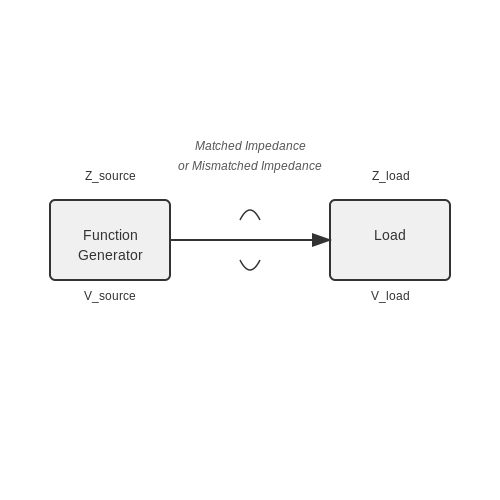
5. Frequency Modulation
5.1 Frequency Modulation
Understanding Frequency Modulation
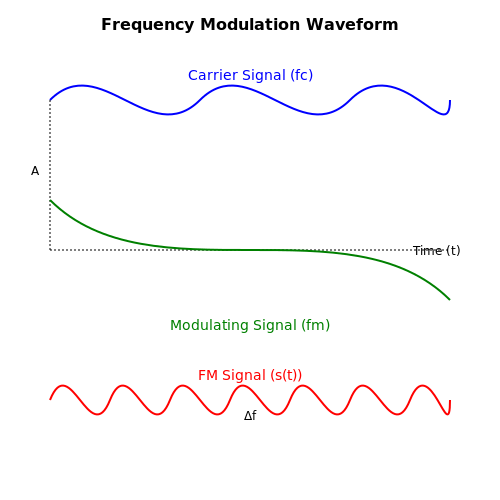
Frequency Modulation (FM) is a powerful technique used in electronics and communications where the frequency of a carrier signal is varied in accordance with the amplitude of the input signal. This contrasts with Amplitude Modulation (AM), which varies the amplitude of the carrier signal. FM is widely utilized in various applications including radio broadcasting, two-way radio communications, and even in some types of data transmission systems.
Mathematical Foundation of Frequency Modulation
To appreciate the implications of frequency modulation, it is essential to grasp its mathematical framework. The general form of an FM signal can be expressed as:
In this equation:
- $$s(t)$$: the modulated FM signal
- $$A$$: the amplitude of the carrier signal
- $$f_c$$: the frequency of the carrier signal
- $$\Delta f$$: the frequency deviation, a measure of how much the carrier frequency varies
- $$f_m$$: the frequency of the modulating signal
This relationship indicates that the instantaneous frequency of the FM signal is determined by the amplitude of the modulating signal.
Deriving the Characteristics of FM
In order to understand how frequency modulation functions, consider the modulation index $$\beta$$:
This parameter plays a significant role in defining the bandwidth and quality of the modulation. The Carson's Rule for estimating the bandwidth ($$BW$$) of an FM signal is expressed as:
The bandwidth provides critical information for system design, especially when it comes to spectral efficiency and avoiding interference with adjacent channels.
Real-World Applications of Frequency Modulation
FM plays a vital role in modern communication systems. For instance, FM radio broadcasting utilizes this technique to improve sound quality and to provide better resilience against noise compared to AM broadcasting. Additionally, frequency modulation is also employed in Phase-Locked Loops (PLLs), which are prevalent in synthesizers and clock generation circuits. Another significant application is in radar and telemetry systems, where FM enables the transmission of information over varying distances without significant loss of data fidelity.
Conclusion: The Importance of FM in Technology
Frequency modulation remains a foundational concept in electronics and communications. Its capacity to produce high-quality audio signals, combined with effective noise rejection and bandwidth efficiency, make it indispensable in various technological domains. Understanding FM is crucial for engineers and researchers alike, as it underpins many modern communication systems.
5.2 Amplitude Modulation
Amplitude Modulation (AM) is a fundamental technique in signal processing, widely used in communications. This method is critical for transmitting information over carrier waves, enabling the transfer of audio, video, and data signals. In essence, AM works by varying the amplitude of a carrier wave in accordance with the information signal.
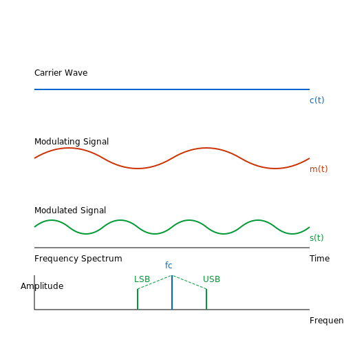
To grasp the intricacies of amplitude modulation, we must first establish a clear understanding of the basic components involved. The process entails combining a modulating signal (which contains the information to be transmitted) with a high-frequency carrier signal. The resultant modulation can be expressed mathematically through a series of derivations that highlight the relationship between the signals.
Understanding the AM Signal
Consider a low-frequency message signal represented by m(t) and a high-frequency carrier wave represented by c(t). The carrier wave can generally be expressed as:
where Ac is the carrier amplitude and fc is the carrier frequency. The modulating signal is described by the function:
where Am denotes the amplitude of the modulating signal and fm is its frequency. In amplitude modulation, the amplitude of the carrier is varied in proportion to the instantaneous value of the modulating signal:
Substituting the expression for m(t) into the equation for s(t), we obtain:
This expression reveals that the resulting AM signal s(t) consists of the original carrier wave at frequency fc and various sidebands created by the modulation process.
Frequency Spectrum of AM Signals
The frequency spectrum of an AM signal is crucial in understanding its bandwidth and the necessity for spectral containment when transmitting over various mediums. When modulating a carrier wave, sidebands are formed at frequencies equal to the sum and difference of the carrier frequency fc and the modulation frequency fm. The resulting frequencies are:
- Upper Sideband (USB): fc + fm
- Lower Sideband (LSB): fc - fm
This modulation process implies that the bandwidth required for an AM signal is twice that of the modulating signal, leading to:
Practically, this delineation allows for efficient allocation of frequency bands in communication systems, especially in radio broadcasts where multiple channels must coexist without interference.
Applications of Amplitude Modulation
As an essential part of electronic communications, amplitude modulation is still prevalent in various domains, such as:
- AM radio broadcasting: The traditional method for transmitting audio signals over long distances.
- Aerospace communications: Used in both civilian and military aircraft for communicating navigation and other telemetry data.
- Television audio transmissions: AM is utilized for embedding audio in video broadcasts, particularly in older analog TV systems.
With the advent of digital communication systems, AM has been complemented by more sophisticated methods, yet it remains a subject of critical study in both theory and practical application due to its inherent simplicity and effectiveness.
5.3 Phase Shift Keying
Phase Shift Keying (PSK) represents a crucial modulation technique widely used in digital communication systems. It enables the transmission of data signals by altering the phase of a carrier wave, providing robustness against signal distortion and noise. This aspect of PSK makes it particularly valuable in environments where high fidelity is paramount, such as satellite communication, digital television, and wireless networking.
Understanding Phase Shift Keying
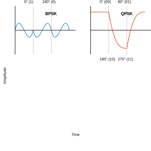
At its core, PSK works by encoding data into discrete phase shifts of a continuous wave signal. For example, in Binary Phase Shift Keying (BPSK), the phase of the carrier wave is shifted by 0 or 180 degrees to represent binary digits (0s and 1s). Similarly, in Quadrature Phase Shift Keying (QPSK), four distinct phase shifts—0, 90, 180, and 270 degrees—allow for the representation of two bits per symbol. This increases the data transmission efficiency without increasing the bandwidth.
The mathematical representation of a PSK signal can be expressed using the following formula:
Where:
- s(t) is the modulated signal.
- A is the amplitude of the carrier wave.
- f_c is the carrier frequency.
- \(\phi\) is the phase shift denoting the transmitted data.
To understand the relationship between phase changes and different data states, let's derive the phase shifts for BPSK and QPSK.
Binary Phase Shift Keying (BPSK)
In BPSK, the phase shift is straightforward:
- For a binary '0': \( \phi = 0 \) degrees.
- For a binary '1': \( \phi = 180 \) degrees.
This leads to two possible signals:
Quadrature Phase Shift Keying (QPSK)
In QPSK, we can group bits into pairs. Assigning them to distinct phases results in four possible combinations:
- 00: \( \phi = 0 \) degrees
- 01: \( \phi = 90 \) degrees
- 10: \( \phi = 180 \) degrees
- 11: \( \phi = 270 \) degrees
Thus, the corresponding signal representations become:
Practical Applications of PSK
PSK has been employed in various real-world applications, primarily due to its resistance to noise and ability to maintain a high data rate. Below are a few notable implementations:
- Wireless Communication: PSK is prevalent in mobile systems and Wi-Fi connections, where robust data transmission is essential.
- Satellite Communication: Delivers reliable transmission in the challenging environment of space.
- Digital Television Broadcasting: Ensures high-quality video and audio streams through effective modulation techniques.
Understanding the principles of PSK and its various forms equips engineers and researchers with fundamental tools for designing efficient communication systems, making it an indispensable area of study in electronics and telecommunications.
6. Calibration Procedures
6.1 Calibration Procedures
Calibration is a crucial process for ensuring the accuracy and reliability of applied function generators in various engineering and research applications. This subsection sheds light on the intricate methodologies and best practices for calibrating these devices, laying the groundwork for high-precision testing and measurement.
Understanding Calibration
Calibration involves comparing the output of a function generator against a recognized standard. This process is essential to quantify deviations, which can stem from factors such as component aging, temperature variations, and inherent device inaccuracies. An accurate calibration enhances the quality of experimental data and ensures that the functions generated are reliable for further analysis or application.
Calibration Protocols
Establishing a robust calibration protocol is key to achieving consistent results. Typically, these steps may include:
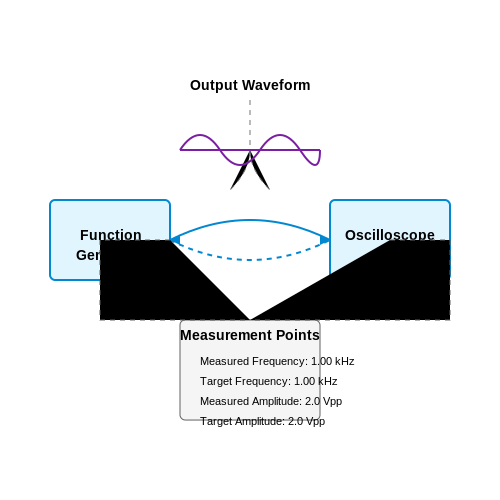
- Prepare Calibration Equipment: Ensure that calibrated measurement instruments, such as oscilloscopes, are available. The accuracy of your reference equipment plays a fundamental role in the calibration process.
- Select Calibration Points: Choose specific output frequencies and amplitudes that represent the intended operational range of the function generator.
- Perform Measurements: Generate a known output and measure it with the calibrated reference instruments. Record the results accurately.
- Analyze Data: Compare the measured output to the expected output to identify discrepancies. This step may involve statistical analysis to evaluate variability.
- Document Calibration: Keep thorough records of calibration results, adjustments made, and any anomalies encountered during testing.
Detailed Steps for Calibration
Let’s dive deeper into specific calibration steps:
1. Equipment Setup
Before beginning the calibration procedure, set up the oscilloscope to ensure that its bandwidth and sample rate are suitable for capturing the function generator's output characteristics. The oscilloscope should be connected to the output of the function generator with appropriate probes.
2. Frequency Calibration
For frequency calibration, follow these steps:
- Generate a sine wave at a target frequency, starting from a low frequency and moving to higher ones.
- Measure the frequency on the oscilloscope and record the result.
- Adjust the function generator to reduce the error, if needed, using the reference standard as a guide.
It is advisable to perform this calibration for multiple distinct frequencies to cover the function generator's entire operational range.
3. Amplitude Calibration
Amplitude calibration verifies that the output voltage matches the specified values:
- Set the function generator to generate a known amplitude at a specific frequency.
- Use the oscilloscope to measure the peak-to-peak voltage of the output waveform.
- Calculate the percentage error using the formula:
$$ \text{Percentage Error} = \left( \frac{\text{Measured Value} - \text{Actual Value}}{\text{Actual Value}} \right) \times 100 $$
- Make necessary adjustments to the output settings on the function generator.
Real-World Implication of Calibration
Effective calibration is often the difference between successful and failed experiments or product designs. For instance, in high-frequency electronics, any deviation in output can lead to degraded performance of RF circuits. Similarly, in automotive testing, incorrect signal generation can lead to faulty diagnostics and consequently increased costs.
The reliability of results obtained from a calibrated function generator translates into technological advancements across numerous fields. This highlights the significance of rigorous calibration as an ongoing process rather than a one-time procedure, ensuring that all outputs remain aligned with precision standards over time.
In summary, robust calibration procedures are indispensable in the realm of applied function generators, involving a systematic approach that not only enhances the accuracy of the instruments but also contributes to the integrity of the scientific process.
6.2 Testing Output Accuracy
In the realm of applied function generators, the accuracy of the output signals produced is paramount to ensure effective experimental results and device functionality. Accurate outputs facilitate precise system responses, making it essential for engineers, physicists, and researchers to evaluate the performance and reliability of these tools rigorously. This section delves into the methodologies for testing output accuracy, including both theoretical insights and practical considerations.Understanding the Basics of Output Accuracy
Output accuracy in function generators refers to the fidelity of the output signal compared to the expected waveform. This can encompass a variety of wave shapes, such as sine, square, triangle, and arbitrary waveforms, each requiring distinct testing procedures. Various metrics can be employed to quantify accuracy, including amplitude, frequency stability, distortion, and phase jitter. A critical concept tied to output accuracy is the notion of signal fidelity. Fidelity measures how accurately the generated signal retains the characteristics of the ideal signal. High fidelity corresponds to minimal distortion and precise amplitude and frequency outputs.Key Parameters for Testing
When evaluating the accuracy of outputs from function generators, consider the following key parameters:- Amplitude Accuracy: This parameter assesses how closely the output voltage matches the set value. Amplitude errors can arise due to calibration mismatches or non-linear behavior of components.
- Frequency Accuracy: Frequency accuracy evaluates how closely the frequency of the output waveform aligns with the intended frequency. This is influenced by the stability of internal clocks and component tolerances.
- Harmonic Distortion: This measures the extent of unwanted frequencies at harmonics of the fundamental frequency. Excessive harmonic distortion can degrade signal clarity and system performance.
- Phase Noise: Phase noise represents rapid, short-term variations in signal phase, which can adversely affect sensitive applications such as communication and signal processing.
Testing Methods and Tools
The evaluation of output accuracy can be conducted through a combination of laboratory equipment and methodologies, which can vary based on the waveform characteristics.1. Oscilloscope Measurements
The most straightforward approach to testing output accuracy is using an oscilloscope. This device allows for real-time visualization of waveforms, enabling users to measure key parameters directly. Consider the following steps when using an oscilloscope: 1. Connect the Oscilloscope: Attach the oscilloscope probes to the output of the function generator. Maintain proper grounding to avoid measurement inaccuracies. 2. Set Trigger Level: Adjust the trigger level to synchronize the waveform display, allowing for a stable view of the signal. 3. Analyze Waveform: Measure amplitude, frequency, and distortion using the oscilloscope’s measurement functions. For harmonic distortion, use the FFT (Fast Fourier Transform) feature to visualize frequency components.2. Multimeter Usage
For straightforward measurements, a digital multimeter can assess both voltage output and frequency accuracy. While it does not provide waveform shape information, it offers a quick assessment of amplitude levels and can measure the frequency of square waves effectively.3. Signal Analyzers
For applications requiring high precision, a signal analyzer serves as an advanced tool for evaluating waveform characteristics, including spectral purity. These devices are particularly useful for RF communications and instrumentation where high fidelity signals are critical.Practical Application Example
Consider a scenario where a researcher is designing a circuit for audio applications that require sine wave outputs with minimal distortion. By employing an oscilloscope for real-time observations, the researcher can adjust the function generator parameters while continuously monitoring output quality. Utilizing a signal analyzer, the researcher further examines harmonic distortion and noise characteristics, ensuring the output signal perfectly aligns with audio fidelity standards. Through diligent testing and evaluation, users can confirm the function generator's output accuracy, confidently integrating it into their experimental setups.Conclusion
In conclusion, the principles of testing output accuracy in function generators are fundamental to achieving successful outcomes in advanced research and engineering applications. By understanding key parameters, employing appropriate tools, and following sound testing protocols, users can ensure their output signals are reliable and effective for their intended purposes.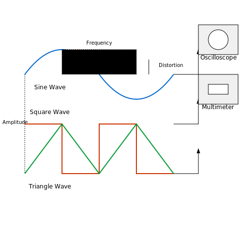
6.3 Troubleshooting Common Issues
Applied function generators are essential tools in electronics and signal processing, but they can present challenges during operation. Whether it's an incorrect output signal, unstable frequency, or unexpected waveform characteristics, understanding how to effectively troubleshoot these common issues is critical for engineers and researchers alike. In this section, we will explore practical troubleshooting strategies, provide insight into potential causes of issues, and offer solutions to restore optimal functionality.
Identifying Common Output Signal Issues
One of the most immediately perceivable issues with function generators is an incorrect output signal. This might manifest as a waveform that differs from the expected shape or undesired frequency deviations.
- Waveform Accuracy: Consider the basic parameters of the generator. Check the waveform settings in your function generator's user interface, ensuring that you have selected the correct type—sine, square, triangle, or sawtooth. You might also need to verify that the amplitude and offset values are set to appropriate levels, as these can dramatically alter the output wave shape.
- Frequency Calibration: Use an oscilloscope to compare the output frequency to a known reference frequency. If discrepancies exist, it may indicate an issue with the internal oscillator's calibration. Many models allow for calibration adjustments, typically accessed in the setup menu of the instrument.
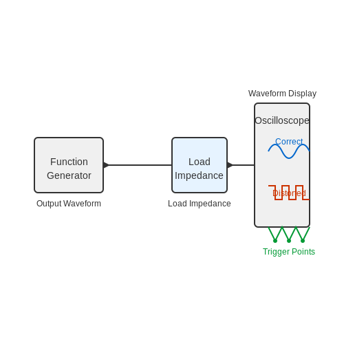
If the waveform appears distorted or clipped, it might indicate that the output has been driven into a non-linear region, possibly due to excessive load. Check the load connected to the generator and ensure that it matches the specified impedance of the output. Avoiding low-impedance loads can significantly enhance waveform integrity.
Diagnosing Stability Problems
Another frequent issue encountered is stability in frequency output. Stability problems can lead to drift in the generated signals, compromising the accuracy of your measurements.
- Temperature and Environmental Effects: Function generators can be sensitive to changes in temperature. Fluctuations in ambient temperature can affect the oscillator frequency. Ensure your generator is operating in a controlled environment where extreme thermal variations are minimized.
- Power Supply Stability: Verify that the power supply is clean and stable. Power supply noise can introduce unwanted fluctuations in the output frequency. Utilize an oscilloscope to monitor the input voltage and check for ripples or transients that may influence output stability.
For DC-coupled devices, small shifts in power supply voltage can modify oscillator performance. Consider adding voltage regulation or conditioning devices between your power source and the function generator.
Evaluating Signal Quality
When your output signal exhibits noise or other artifacts, assessing the signal quality should be a priority.
- Verify Cabling and Connections: Electrical noise can often be attributed to faulty or poorly shielded cables. Ensure that BNC connectors are secure and cables are intact. Additionally, using twisted pair cables can help to eliminate external electromagnetic interference.
- Grounding Issues: Ensure the function generator is properly grounded. Ground loops or poor grounding can introduce noise into the output signal. Consider the grounding schemes of associated equipment when troubleshooting.
Lastly, employing high-frequency probes can help isolate where the noise may be entering the system. By systematically analyzing different sections, you can pinpoint and mitigate the sources of interference.
Understanding Output Load Limitations
Finally, each function generator has inherent output limitations that must be respected to avoid damaging the unit or producing low-quality signals. Always refer to the manufacturer’s specifications regarding output voltage, current, and load impedance.
- Load Impedance Matching: If the connected load significantly deviates from the recommended impedance, the function generator may produce incorrect waveform characteristics. Use an appropriate load, as specified in the user manual, to ensure that the output remains stable and reliable.
- Overcurrent Protection: Many function generators incorporate built-in protection features to safeguard against overcurrent situations. Familiarize yourself with these functions; misunderstandings may lead to inadvertent unit shutdowns or damage.
By attending to these common issues with awareness and systematic analysis, you can enhance both your understanding of function generators and your ability to operate them effectively. As you gain experience, troubleshooting will become not just a necessity, but also an opportunity for deeper learning and exploration within your field.
7. Signal Simulation in Circuit Design
7.1 Signal Simulation in Circuit Design
Signal simulation plays a crucial role in modern circuit design by enabling engineers and researchers to model and analyze circuit behavior before physical implementation. This practice not only saves time and resources but also facilitates an in-depth understanding of circuit performance under varying conditions. An applied function generator is central in this process, capable of producing a diverse range of waveforms for testing and validation.
Understanding Signal Waveforms
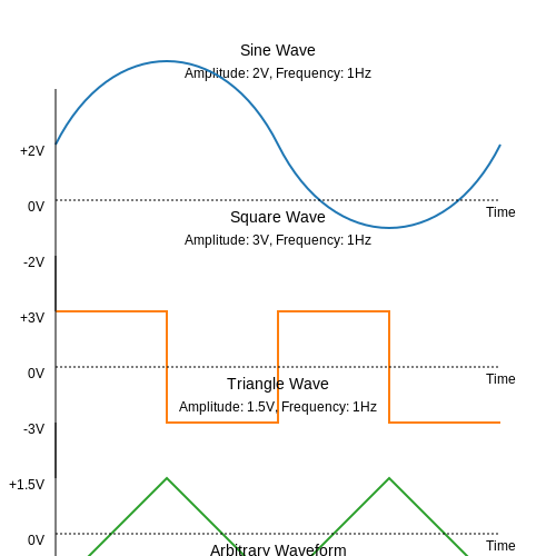
Commonly generated signal waveforms include sine, square, triangle, and arbitrary waveforms. Each of these serves different purposes:
- Sine Waves: Often used to represent AC signals, they are ideal for linearity tests.
- Square Waves: Useful in digital circuits for timing analysis and switching behavior.
- Triangle Waves: Employed in various control applications, they are both linear and easy to integrate.
- Arbitrary Waveforms: Custom shapes tailored to simulate realistic scenarios, enhancing the fidelity of circuit testing.
By analyzing these waveforms, designers gain insights into a circuit's frequency response, distortion, and transient behavior. This is where applied function generators excel, providing flexibility and precision in waveform generation.
Mathematical Modeling of Waveforms
A fundamental aspect of signal simulation is mathematically modeling the waveforms produced. For instance, consider a sine wave represented by the function:
Where:
- V(t): instantaneous voltage at time t
- V0: amplitude of the signal
- f: frequency in hertz
- φ: phase shift in radians
Understanding the parameters that define these waveforms enables the precise tuning of function generators. For example, adjusting the amplitude V0 affects the signal's output voltage, while changing the frequency f allows exploration across the response spectrum of the circuit under test.
Application in Circuit Design
In circuit design, simulated signals using function generators provide essential insights. For instance, during the testing phase of a radio frequency (RF) circuit, a function generator might output a range of frequencies enabling a designer to measure parameters such as gain, bandwidth, and linearity. By systematically varying signal characteristics, designers gauge the circuit’s response, identifying any potential issues before production.
Moreover, in the realm of digital signal processing (DSP), function generators mimic real-world signals, facilitating algorithm testing in an environment analogous to actual operational conditions. This ensures that the software operates correctly before being paired with hardware.
Conclusion
Signal simulation through applied function generators is integral to modern circuit design. The ability to model and generate specific waveforms allows for extensive testing and validation, ultimately leading to improved circuit performance, reliability, and efficiency. As technology advances, the capabilities of function generators continue to expand, providing engineers with increasingly sophisticated tools for their design challenges.
7.2 Testing Amplifiers and Filters
The testing of amplifiers and filters is an essential aspect in the realm of applied function generators. The performance of these components directly impacts the fidelity and quality of electronic signals, making their analysis pivotal for engineers and researchers. In this section, we will delve into the methodologies and tools required for testing, elucidate the underlying principles, and explore practical applications.
Understanding Amplifiers
Amplifiers are devices that increase the voltage, current, or power of a signal, enabling weak signals to be processed effectively. The fundamental characteristics of an amplifier include gain, bandwidth, and linearity. Gain, often expressed in decibels (dB), indicates how much the amplifier increases the input signal. The bandwidth, defined as the range of frequencies over which the amplifier operates effectively, is crucial for applications involving high-frequency signals.
Testing Amplifiers involves various parameters that must be measured to determine performance. These include:
- Voltage Gain: Measured as the ratio of the output voltage to the input voltage.
- Input and Output Impedance: Determines how the amplifier interacts with preceding and following stages.
- Phase Shift: Particularly important in feedback systems, as it can affect stability.
- Noise Figure: Represents the degradation of the signal-to-noise ratio (SNR) due to the amplifier.
Testing methods often involve the use of network analyzers, oscilloscopes, and signal generators. A typical setup may include a function generator producing a known waveform, which is then fed into the amplifier. The output can be monitored using an oscilloscope to analyze the gains and distortions introduced by the amplifier.
Filter Characteristics and Testing
Filters are paramount in signal processing for allowing or rejecting specific frequency bands. They can be categorized into several types: low-pass, high-pass, band-pass, and band-stop filters. Each type serves distinct purposes in signal conditioning.
Understanding the transfer function is essential, as it describes how the filter alters different frequency components of the input signal. The transfer function \( H(s) \) for a simple low-pass filter, for instance, can be described by:
where \( R \) is the resistance, \( C \) is the capacitance, and \( s \) is the complex frequency variable. This equation illustrates how the output is affected as frequency increases, eventually leading to a cutoff frequency defined by \( f_c = \frac{1}{2\pi RC} \).
Conducting Filter Tests
To test filters, you typically employ a function generator to apply a range of frequencies at the input. The output is then analyzed using spectrum analyzers. Key performance indicators include:
- Cutoff Frequency: Identifying the frequency at which gain drops to -3 dB.
- Passband Ripple: The variation within the passband, which can indicate filter quality.
- Stopband Attenuation: The effectiveness of the filter in rejecting unwanted frequencies.
- Phase Response: Important for systems where timing is critical.
Real-world applications abound for amplifiers and filters, from telecommunications to audio engineering. For instance, in telecommunications, amplifiers are crucial for extending signal range, while filters mitigate interference, ensuring clearer communication signals.
In summary, effective testing of amplifiers and filters not only requires understanding their theoretical background and operational principles but also employing suitable measurement techniques. Mastery of these concepts is fundamental for any advanced practitioner in electrical engineering and electronics.
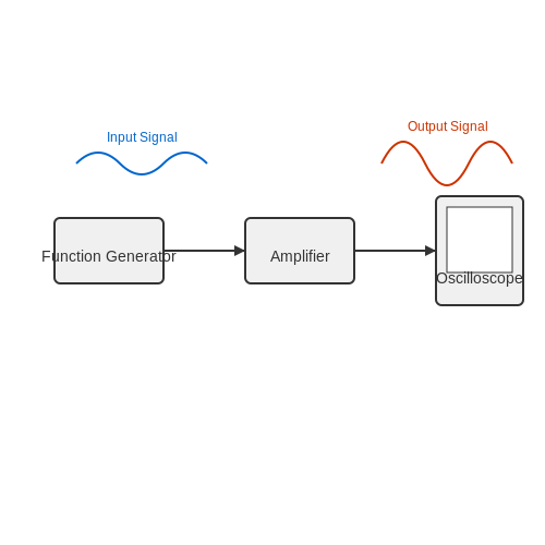
7.3 Using Function Generators in Research
Function generators serve as indispensable tools in research across various scientific domains, providing a stable, precise means of generating electrical waveforms. This subsection explores the diverse applications of function generators in research, emphasizing their practical relevance, underlying physics, and the technical nuances that contribute to their effectiveness.
Waveform Generation and Signal Synthesis
At the core of a function generator's utility is its ability to produce various waveform outputs—such as sine, square, triangle, and sawtooth waves. Each waveform exhibits unique properties, making them suitable for specific research applications. For example, sine waves are often utilized in communication systems and control theory, where pure harmonic signals allow the testing of linear systems.
To illustrate, the mathematical expression for a sinusoidal waveform can be represented as:
where:
- V(t) is the instantaneous voltage.
- V0 is the peak voltage.
- f represents the frequency of the waveform.
- t is time.
- φ is the phase shift.
This equation highlights how the frequency and amplitude can be easily manipulated to match experimental requirements, enabling researchers to emulate real-world scenarios effectively.
Research Applications in Modulation and Testing
In various realms, such as telecommunications and electronics testing, function generators facilitate modulation techniques essential for signal processing. For instance, in amplitude modulation (AM), the function generator creates a carrier signal, which is then modulated by an information signal. The amplitude modulation equation is given by:
where:
- Vc is the carrier signal amplitude.
- Vm is the amplitude of the modulating signal.
- fm is the modulating frequency.
- fc is the carrier frequency.
This capability to simulate various modulation patterns significantly enhances the testing accuracy of receivers and communication devices, ensuring they function correctly under different conditions.
Characterizing Component Behavior
Function generators also play a critical role in characterizing the behavior of electronic components. By applying specific waveforms to devices such as resistors, capacitors, and inductors, researchers can observe and measure their responses. The resulting data aids in understanding frequency response, phase shift, and time constants, which are crucial for system modeling.
For instance, one might apply a square wave signal across a resistor-capacitor (RC) circuit to analyze the voltage response. The behavior can be mathematically predicted using the time constant (τ) defined as:
This relationship indicates how quickly a capacitor charges and discharges, allowing researchers to verify component specifications and performance under various stimuli.
Real-World Case Studies
Numerous studies highlight the effectiveness of function generators in real-world applications. A notable case involves a team utilizing a function generator to analyze the response of photonic devices in optical communications. By generating complex waveforms, the researchers successfully determined bandwidth limitations and optimal operation conditions for laser diodes, contributing to advancements in data transmission technologies.
In essence, function generators are versatile tools that enhance research capabilities across disciplines. Their precision and configurability ensure that they remain integral to experimental setups, offering reliable data for advancing scientific knowledge.
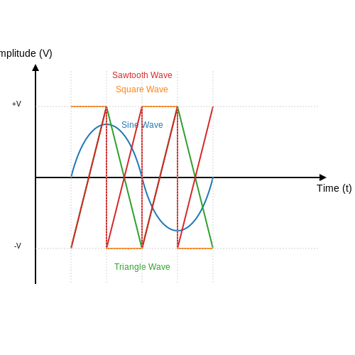
8. Recommended Textbooks
8.1 Recommended Textbooks
- Electronic Instrumentation and Measurement Techniques by W. D. Cooper and A. D. Helfrick — A comprehensive guide offering detailed insights into electronic measurement and instrumentation, including function generators. Its methodical approach to principles and practices serves well for deep academic study.
- Measurement, Instrumentation, and Sensors Handbook by John G. Webster — Provides a complete overview of various instrumentation and sensor technologies with clear explanations of function generator applications in different fields.
- Electronic Components and Technology by Stephen Sangwine and Oliver Faust — This textbook covers electronic components in modern applications, highlighting advanced techniques ideal for professionals, including the use of function generators to test and simulate real-world electronics.
- Introduction to Instrumentation and Measurements by Robert B. Northrop — Offers an introduction to measurement techniques and uses of different instruments. This book is pivotal for understanding modern instrumentation and the context of function generators in scientific research.
- Principles of Electronic Instrumentation and Measurement by Howard M. Berlin — Focuses on the principles underlying the operation of electronic instrumentation, including coherent sections on deploying function generators in measurement systems.
- Fundamentals of Instrumentation and Measurement by Dominique Placko — This book provides a fundamental yet thorough examination of instrumentation systems, with practical examples of using function generators across various electronic fields.
- Electronic Instrumentation by H. S. Kalsi — With detailed explanations on various electronic instruments, this reference is specially tailored for understanding the technical nuances and applications of function generators in industry.
8.2 Online Resources
- Tektronix Function Generator Basics — A comprehensive guide by Tektronix discussing function generator fundamentals, operation principles, and practical applications for engineers and physicists.
- Keysight Function and Waveform Generators — High-quality resources detailing various function generator models, with specifications and recommended use cases from Keysight Technologies.
- What is a Function Generator? — Circuit Specialists provide insights into the types, uses, and importance of function generators in electronics testing and research environments.
- Function Generator FAQ — A useful FAQ section offering detailed answers to common questions about function generators and their applications in circuit design and testing.
- Versatile Function Generators Ease the Task of Test & Measurement — Electronic Design explores the flexibility and capabilities of modern function generators in test and measurement settings.
- Function Generators Explained — Brüel & Kjær's well-detailed article explaining the methodologies behind function generation, including practical guidelines for engineers.
- Module: Function Generators — Delft University of Technology offers a module for advanced users looking to delve deeper into the theory and practical deployment of function generators.
- Function Generators: What You Need to Know Before Buying — A buyer's guide that covers factors to consider when purchasing a function generator for professional testing applications.
8.3 Research Articles
- Design and Implementation of Function Generators — An IEEE paper discussing the design methodologies and practical implementation of function generators, highlighting the engineering challenges and solutions.
- Precision Function Generators in Scientific Research — This study explores the role of high-precision function generators in scientific experimentation, emphasizing their importance in accurate signal generation.
- An Overview of Modern Function Generators — This article provides insights into the advancements and modern developments in the function generator technology, focusing on innovation in signal processing.
- Integration of Function Generators with Digital Platforms — Examine how digital technology enhances the capabilities of traditional function generators, including integration with modern digital systems for enhanced functionality.
- Advancements in Arbitrary Function Generators — This research article discusses technical improvements and innovative features in arbitrary function generators, which offer flexibility in waveform synthesis.
- Utilization of Function Generators in Electromagnetic Experiments — Discusses the application of function generators in the field of electromagnetism, providing case studies on their use in experimental setups and data validation.
- Measurement: A Journal on Function Generators and Evaluation — This journal covers comprehensive reviews and studies on the evaluation and testing of function generators, offering critical insights into performance metrics.