Electrical Waveforms

#electrical waveforms #sinusoidal #square wave #triangular wave #sawtooth wave #pulse wave #amplitude #frequency #waveform parameters

1. Definition of Electrical Waveforms

1.1 Definition of Electrical Waveforms

Electrical waveforms represent the variations in electrical parameters, such as voltage, current, or power, as they change over time. These waveforms are fundamental to the interpretation and understanding of electronic systems, encompassing a broad range of shapes and characteristics that can be described mathematically. To truly grasp electrical waveforms, we must appreciate their significance across various applications in physics and electronics, particularly in signal processing, communication systems, and power engineering.

Understanding Waveforms in Electrical Context

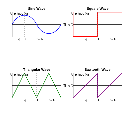
At its core, an electrical waveform is a graphical representation of an electrical signal's variation over time. The two primary types of waveforms are periodic and aperiodic. Periodic waveforms repeat at regular intervals and include sine, square, triangular, and sawtooth shapes. In contrast, aperiodic signals, such as random noise, do not exhibit regular repeating patterns.

Characteristics of Electrical Waveforms

Each waveform can be characterized by several parameters including:

Amplitude (A): The maximum value of the waveform, representing the strength of the signal.
Frequency (f): The number of cycles (or repetitions) per second, measured in Hertz (Hz).
Period (T): The time duration of one complete cycle, related to frequency by the equation T = 1/f.
Phase (φ): A measure of the position of the waveform cycle at a specified time, often expressed in degrees or radians.

Mathematical Representation

Mathematically, waveforms can be expressed using functions. The most common form is the sine wave, described by the equation:

$$ V(t) = A \sin(2\pi f t + φ) $$

Here, V(t) indicates the voltage at time t, while A, f, and φ represent the amplitude, frequency, and phase, respectively. This equation encapsulates the model for periodic signals, allowing for variations that can be dictated by the specific application. For instance, in communication systems, sine waves can be modulated to encode information effectively.

To further illustrate this relationship, let’s derive the expression for a square wave, which can be defined as alternating between two levels, with equal intervals of high and low potential. Its mathematical representation is given by:

$$ V(t) = \begin{cases} A & \text{for } 0 \leq t < T/2 \\ -A & \text{for } T/2 < t < T \end{cases} $$

Such a square waveform is especially valuable in digital electronics, where it symbolizes binary states (0 and 1), forming the foundation for logic circuits and switching systems.

Practical Applications of Electrical Waveforms

The study of electrical waveforms is essential in numerous fields:

Signal Processing: Engineers analyze various waveforms to extract information and ensure signal integrity in telecommunications.
Power Systems: Waveforms inform the design and stability of AC power systems, influencing how energy is distributed and utilized.
Medical Devices: Waveform analysis is critical for interpreting signals in medical imaging technologies and patient monitoring systems.
Audio Engineering: Understanding waveforms allows for better sound manipulation and effects processing in music production.

In conclusion, electrical waveforms serve as a crucial foundation in both theoretical and practical aspects of engineering and physics. By incorporating mathematical rigor and analyzing their attributes, we can devise solutions and innovations that impact multiple domains, ranging from consumer electronics to industrial applications.

Definition of Electrical Waveforms in Electrical Waveforms

Diagram Description: The diagram would visually illustrate the different types of electrical waveforms (sine, square, triangular, sawtooth) along with their key characteristics (amplitude, frequency, and phase) to enhance understanding. This representation can clarify their periodic and aperiodic nature, showing their time-domain behavior more effectively than text alone.

1.2 Importance of Waveforms in Electronics

Understanding electrical waveforms is fundamental to the design, analysis, and application of electronic systems. Waveforms convey critical information about signal characteristics such as frequency, amplitude, phase, and shape, which serve as the basis for various applications in electronics.

From the simplest circuits to complex digital communication systems, the shape and nature of waveforms can drastically alter the performance and functionality of an electronic design. For instance, in digital communication, waveform characteristics are essential for error detection, signal integrity, and overall transmission efficiency. A clear distinction between different waveforms allows engineers to achieve better data representation and modulation. This is particularly important in the context of time-division multiplexing (TDM), where multiple data streams are combined into one signal over a shared medium.

1.2.1 Frequency and its Implications

The frequency of a waveform has profound implications for its real-world applications. In alternating current (AC) circuits, for example, the frequency dictates not only the behavior of the circuit components but also how efficiently energy is transferred. High-frequency signals are often used in radio transmission, where smaller wavelengths allow for more efficient antenna size and improved data throughput.

Moreover, consider the scenario of signal filtering. Depending on the waveform's frequency, different filtering techniques can be applied. Low-pass filters will allow low-frequency signals to pass while attenuating higher frequencies, which is crucial in audio electronics to eliminate high-frequency noise. Conversely, high-pass filters serve the opposite purpose, making them invaluable in eliminating low-frequency noise in communication systems.

1.2.2 Amplitude and Signal Strength

The amplitude of a waveform is directly related to its signal strength. A higher amplitude indicates a stronger signal, which can improve communication reliability, particularly in wireless systems. However, it's crucial to balance amplitude levels to avoid distortion; excessively high amplitudes can lead to clipping, where the waveform's peaks are truncated. This is often seen in audio electronics and digital signals, necessitating the use of techniques such as automatic gain control (AGC) to maintain signal integrity.

For instance, in pulse-width modulation (PWM) applications, the amplitude can be varied to represent different voltage levels, thereby controlling motor speeds or LED brightness. Understanding the relationship between amplitude and power consumption is essential for optimizing electronic designs, particularly in battery-powered devices.

1.2.3 Waveform Shape and Its Impact

The shape of the waveform provides insights into the operation of the underlying electronic components. For example, sine waves are ideal for signaling in AC power systems due to their smooth variation, while square waves are used in digital circuits due to their binary nature. More complex waveforms can arise in scenarios where non-linear components are involved, leading to phenomena such as harmonics and intermodulation distortion. Fourier analysis is commonly employed to decompose these complex waveforms into their fundamental frequencies, aiding in the design and analysis of filters and amplifiers.

As such, understanding how waveform shape affects performance is crucial in applications ranging from audio signal processing to radio frequency (RF) transmission. For instance, in digital signal processing (DSP), engineers rely heavily on specific waveform shapes for effective data encoding and error correction, underscoring the critical role of waveforms in modern electronics.

In summary, the importance of waveforms in electronics cannot be overstated. Their characteristics—frequency, amplitude, and shape—are pivotal across numerous applications in signal processing, communication, and control systems. Mastering these concepts not only helps engineers design more efficient electronic devices but also equips researchers and physicists to explore new frontiers in technology.

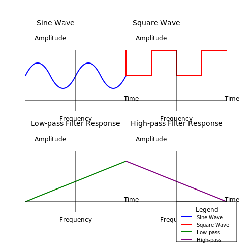
Importance of Waveforms in Electronics in Electrical Waveforms

Diagram Description: The diagram would illustrate the relation between frequency, amplitude, and shape of different waveforms, showing how they interact within electronic applications. This would visually clarify the distinct characteristics and implications of each aspect discussed in the text.

1.3 Basic Concepts of Waveforms

In the study of electrical waveforms, one must first understand the foundation upon which these waveforms are built. Waveforms represent the variation of a quantity (typically voltage or current) over time, and they play a critical role in a multitude of applications, from signal processing to power electronics. To appreciate the profound implications of waveforms, we must explore their fundamental characteristics, categories, and mathematical representations.

Waveform Characteristics

Waveforms can be characterized by several fundamental properties, which define their behavior and performance. 1. Amplitude: This refers to the maximum extent of a waveform's value from its mean position. In a voltage waveform, amplitude indicates the peak voltage, which directly affects power delivery in circuits. 2. Frequency: This is the number of cycles a waveform completes in one second, measured in Hertz (Hz). Frequency determines the behavior of waveforms in communication systems, influencing bandwidth and data transfer rates. 3. Period: The period is the duration taken to complete one full cycle of the waveform. It is inversely related to frequency, calculated as $ T = \frac{1}{f} $, where $ T $ is the period and $ f $ is the frequency. 4. Phase: This property indicates the position of the waveform relative to a reference point in time, expressed in degrees or radians. Phase relationships are crucial in AC circuits, where the synchronization of multiple waveforms can significantly impact system performance. Understanding these characteristics lays the groundwork for analyzing more complex waveforms and understanding their behavior in various applications.

Types of Waveforms

Waveforms can be broadly categorized into two types: continuous and discrete. However, the most common classifications are based on their shape and behavior, primarily:

Sinusoidal Waveforms: These periodic waveforms are smooth and repetitive, resembling the sine function. They are the foundation of alternating current (AC) circuits, representing pure frequency with a single frequency component. Sinusoidal waveforms are vital in power generation and transmission, where they minimize energy loss in resistive loads.
Square Waveforms: Characterized by their abrupt transitions between high and low states, square waveforms have a 50% duty cycle, meaning they spend equal time in the high and low states. They are instrumental in digital electronics and signal processing, acting as clock signals in circuits to synchronize operations.
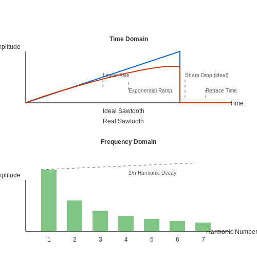
Sawtooth Waveforms: These waveforms increase linearly and sharply return to their starting point, resembling the teeth of a saw. They are often used in audio synthesizers and other electronic devices where linearly varying signals are needed.
Triangular Waveforms: Similar to sawtooth waveforms but with a linear rise and fall, triangular waveforms are used in modulation techniques and audio applications. Their smooth transitions minimize sudden changes in signal, reducing electromagnetic interference.

Each type of waveform offers unique advantages and is chosen based on the application's specific requirements.

Mathematical Representation of Waveforms

To rigorously analyze waveforms, it’s often necessary to express them mathematically. For example, a sinusoidal waveform can be represented as:

$$ V(t) = V_{max} \sin(2\pi f t + \phi) $$

where: - $ V(t) $: instantaneous voltage at time $ t $, - $ V_{max} $: peak voltage (amplitude), - $ f $: frequency, - $ \phi $: phase angle in radians. As a more complex example, the Fourier series allows us to express any periodic waveform as a sum of sinusoidal components, enabling analysis in the frequency domain:

$$ f(t) = a_0 + \sum_{n=1}^{\infty} (a_n \cos(2\pi nft) + b_n \sin(2\pi nft)) $$

where $ a_0 $, $ a_n $, and $ b_n $ are the Fourier coefficients, determining the amplitude of each frequency component in the waveform. This representation is particularly useful in signal processing and communications, allowing engineers to tailor signal characteristics for optimal performance.

Applications of Waveforms

The understanding of waveforms transcends mere academic curiosity; it translates into practical applications across various fields: - Power Distribution: Sinusoidal waveforms are pivotal in AC power systems, minimizing losses and ensuring compatibility with inductive and capacitive loads. - Signal Processing: Square and triangular waveforms are fundamental in digital communication systems, where signal integrity is paramount. - Audio Technology: Waveforms are manipulated in synthesizers to create and modulate sounds, influencing everything from musical production to sound design in film. - Control Systems: Frequency analysis of waveforms is essential in control systems, where feedback mechanisms rely on precise waveform characteristics for stability. In conclusion, a deeper exploration of the basic concepts surrounding electrical waveforms provides a solid foundation for more advanced topics in the field of electronics. Understanding the nuances of waveform properties, types, mathematical representations, and real-world applications is vital for any advanced practitioner in the field.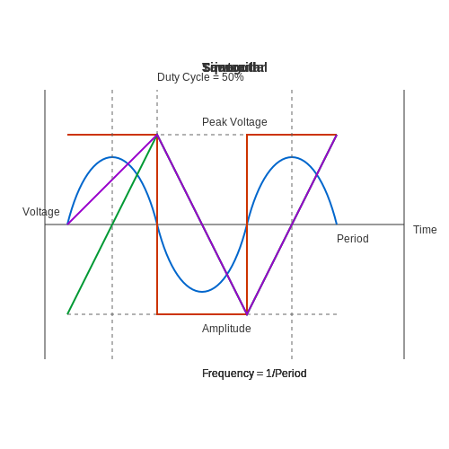

Basic Concepts of Waveforms in Electrical Waveforms

Diagram Description: The diagram would physically show the four types of waveforms (sinusoidal, square, sawtooth, triangular) along with their key characteristics (amplitude and period) visually represented to enhance understanding of their shapes and differences.

2. Sinusoidal Waveforms

2.1 Sinusoidal Waveforms

Sinusoidal waveforms form the foundational waveform in electrical engineering and physics, aiding in the analysis of alternating current (AC) systems, signal processing, and communication technologies. Characterized by their smooth periodic oscillations described mathematically by the sine and cosine functions, these waveforms have distinctive features that allow for various real-world applications.

Mathematical Representation

The sinusoidal waveform can be expressed in two common forms: the sine and cosine functions. The general mathematical representation is given by:

$$ f(t) = A \sin(\omega t + \phi) $$

Where:

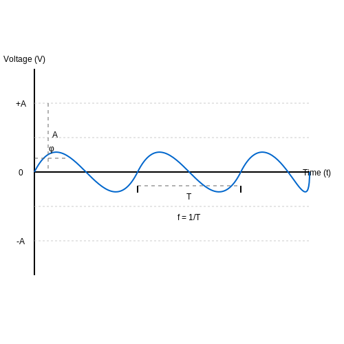
A represents the amplitude of the waveform, determining the peak value.
$\omega$ (the angular frequency) is defined as $ \omega = 2 \pi f $, where f is the frequency of the wave.
t denotes time.
$\phi$ is the phase shift, illustrating the horizontal displacement of the waveform.

Key Characteristics of Sinusoidal Waveforms

Sinusoidal waveforms have several critical characteristics that highlight their significance:

Period (T): The duration of one complete cycle, given by $ T = \frac{1}{f} $.
Frequency (f): The number of cycles per unit time, measured in hertz (Hz).
Amplitude (A): The maximum deviation from the mean value, representing the energy carried by the wave.
Phase Shift ($\phi$): The angle by which the waveform is shifted horizontally, critical in applications requiring synchronization.

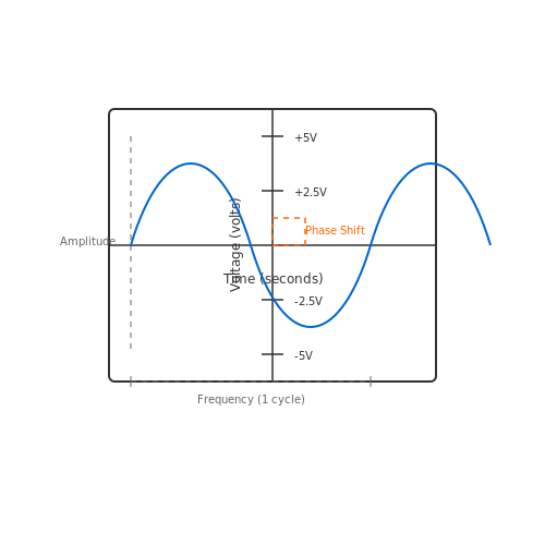
Visualizing a sinusoidal wave provides insight into its properties. Typically, the waveform appears as a smooth sinusoidal curve, oscillating above and below the zero voltage level. The peaks or troughs represent the positive and negative amplitudes, respectively, while the x-axis denotes time and the y-axis represents voltage or current.

Applications of Sinusoidal Waveforms

Sinusoidal waveforms are prevalent across multiple domains, including:

Power Generation: Used in AC power systems to transmit electricity efficiently over long distances.
Communication Systems: Employed in modulation techniques such as amplitude modulation (AM) and frequency modulation (FM).
Signal Processing: Integral to Fourier analysis, enabling the decomposition of complex signals into simpler sinusoidal components.

In engineering, the analysis of systems often utilizes the sinusoidal steady-state response to evaluate circuit behavior under sinusoidal inputs. The transfer functions derived from these sinusoidal waves allow engineers to predict stability and resonance behavior in linear time-invariant systems.

Conclusion

Understanding sinusoidal waveforms is essential for engineers and physicists alike, forming the basis for more complex signal behaviors and circuit analysis. As we proceed to explore more intricate waveforms, the foundational knowledge of sinusoidal functions will remain pivotal in grounding subsequent discussions.

Sinusoidal Waveforms in Electrical Waveforms

Diagram Description: The diagram would visually represent a sinusoidal waveform, showing its amplitude, period, frequency, and phase shift. This representation would clarify the key features of the waveform and its mathematical relationships.

2.2 Square Waveforms

Square waveforms are a fundamental type of periodic waveform characterized by their distinct 'on' and 'off' states, which switch instantaneously between two voltage levels. Unlike sine waves, square waves possess a non-continuous waveform consisting of sharp transitions, making them essential in various applications, notably in digital electronics, signal transmission, and clock generation.

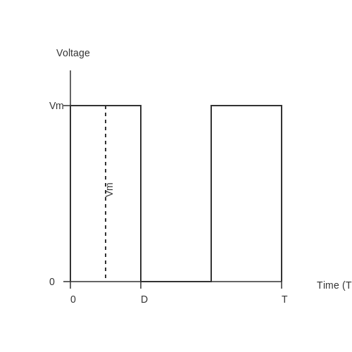
The typical square waveform can be analyzed through its mathematical representation, where it is often defined by its amplitude $ V_m $, frequency $ f $, and duty cycle. The duty cycle represents the proportion of the period during which the signal is in a high state. Specifically, if a square wave has a duty cycle of $ D $, its mathematical representation can be described as follows:

$$ V(t) = \begin{cases} V_m & \text{for } 0 \leq t < D \cdot T \\ 0 & \text{for } D \cdot T \leq t < T \end{cases} $$

Now, let us break down the formula to highlight the aspects of the square waveform. The function denotes that for a fraction $ D $ of the period $ T $, the voltage is at maximum amplitude $ V_m $ while for the remaining portion of the cycle, it returns to zero. This distinctive behavior is visually represented as follows:

In examining the properties of square waves, their Fourier series representation is particularly beneficial since this expands any periodic function into a series of sine and cosine functions. The Fourier series for a square wave can be represented as:

$$ V(t) = \frac{4V_m}{\pi} \sum_{n=1}^{\infty} \frac{1}{2n-1} \sin(2\pi(2n-1)ft) $$

This series reveals that square waves consist not only of their fundamental frequency but also include odd harmonics that contribute to the overall signal. The presence of these harmonics explains the rich spectrum observed when square waves are generated experimentally.

Practical Applications of Square Waveforms

Square waveforms find wide-ranging applications across various domains:

Digital Electronics: Square waves serve as clock signals that synchronize operations in digital circuits, enabling effective data transmission and processing.
Signal Generation: Many testing and functional devices utilize square waves to generate signals for analysis, forming the baseline for observing signal behavior under different conditions.
Inverter Circuits: In power electronics, square waves are often employed in inverter designs to transform DC into AC power by modulating the output waveform.

Historically, advances in the generation and analysis of square waveforms have paved the way for innovations in telecommunications, embedded systems, and modulated signal applications. Understanding the nature of square waveforms not only enhances design capabilities but also accelerates development in cutting-edge technologies.

Conclusion

In summary, square waveforms are integral to modern electronics and signal processing, characterized by their distinct structure. Their mathematical representation, frequency analysis, and practical applications highlight their importance across various scientific and engineering domains.

Square Waveforms in Electrical Waveforms

Diagram Description: A diagram is necessary to visually represent the instantaneous transitions of a square waveform between its 'on' and 'off' states, along with the duty cycle and amplitude. This visualization would clarify the relationship between time (T), duty cycle (D), and voltage (Vm) in a way that text alone does not fully convey.

2.3 Triangular Waveforms

Triangular waveforms are crucial in various engineering applications, particularly in signal processing, communication systems, and waveform generation. This section delves into the characteristics, mathematical properties, and practical applications of triangular waveforms.

Understanding Triangular Waveforms

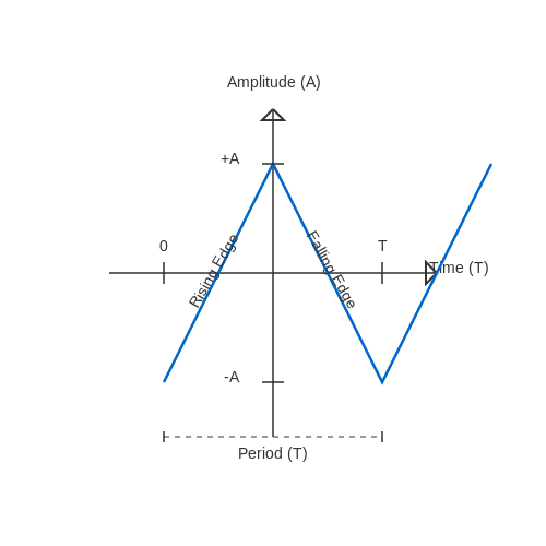
A triangular waveform is a non-sinusoidal waveform named for its triangular shape. It is characterized by linear rising and falling slopes, resulting in a waveform that alternates between maximum and minimum amplitude in a periodic manner.

Mathematically, a triangular waveform can be described as a piecewise function. The waveform can be defined by its period $ T $, amplitude $ A $, and the starting point in its cycle. For a complete cycle, the waveform rises from $-A$ to $A$ over a period defined as $ T/2 $ and then declines back to $-A$ in the next $ T/2 $.

Mathematical Representation

To derive the mathematical expression for a triangular waveform, we need to define its behavior over one complete cycle. The triangular waveform can be expressed in terms of time $ t $ as follows:

$$ x(t) = \begin{cases} \frac{4A}{T}t - A & \text{for } 0 \leq t < \frac{T}{2} \\ -\frac{4A}{T}t + 3A & \text{for } \frac{T}{2} \leq t < T \end{cases} $$

In this expression:

A is the peak amplitude of the waveform.
T is the period of the waveform.

For inverse representations, we can also express the triangular waveform using Fourier series, allowing us to analyze its frequency components:

$$ x(t) = \frac{8A}{\pi^2} \sum_{n=1,3,5}^{\infty} \frac{(-1)^{(n-1)/2}}{n^2} \sin\left(\frac{2\pi n}{T} t\right) $$

Key Characteristics

Triangular waveforms exhibit several remarkable characteristics, including:

Symmetry: The waveform is symmetric about the horizontal axis, enabling easy Fourier analysis.
Harmonic Content: The triangular waveform contains only odd harmonics, decaying in amplitude as the frequency increases.
Rising and Falling Edges: The transition times between maximum and minimum values are linear, allowing easy digital implementations.

Practical Applications

Triangular waveforms find numerous applications in the real world:

Signal Generation: They are used in function generators to create test signals in laboratories.
Communication Systems: Triangular waveforms can modulate signals for amplitude modulation (AM) and frequency modulation (FM).
Audio Synthesis: In synthesizers, triangular waves contribute to a rich sound palette, often used in the production of musical tones.
Control Systems: The smooth transitions of triangular waveforms facilitate linear control actions in electronic feedback systems.

Understanding triangular waveforms is essential for engineers and physicists, as it bridges the gap between theoretical analysis and practical implementation in a wide variety of fields.

Triangular Waveforms in Electrical Waveforms

Diagram Description: The diagram would illustrate the shape of a triangular waveform, showing its linear rising and falling edges over a complete cycle, as well as its amplitude and period. This visual representation would clarify the mathematical description and characteristics discussed in the text.

2.4 Sawtooth Waveforms

The sawtooth waveform is a unique electrical signal characterized by its linear rise and abrupt fall, resembling the teeth of a saw. This shape is prominent in various applications ranging from audio synthesis to television signals and even in timing circuits. Understanding the behavior and mathematical properties of sawtooth waveforms can significantly enhance their utilization in engineering and applied physics.

Mathematical Representation

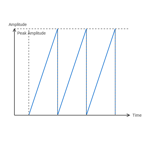
A sawtooth waveform can be described mathematically as a periodic function with a linear rise followed by an immediate drop. This can be captured using the following piecewise function:

$$ f(t) = \begin{cases} \frac{t}{T} & 0 \leq t < T \\ 0 & T \leq t < 2T \end{cases} $$

Here, T represents the period of the waveform. This function exemplifies a linear increase from 0 to 1 over the duration of one period, followed by a return to 0.

Fourier Series Representation

To analyze the harmonic content of a sawtooth waveform, one may employ Fourier series expansion. The Fourier series representation is beneficial in understanding how each harmonic contributes to the overall waveform.

The general formula for the Fourier series of a periodic function can be expressed as:

$$ f(t) = a_0 + \sum_{n=1}^{\infty} \left( a_n \cos\left(\frac{2\pi nt}{T}\right) + b_n \sin\left(\frac{2\pi nt}{T}\right) \right) $$

For a sawtooth waveform, it has been determined that:

$$ a_0 = 0 $$
$$ a_n = 0 $$ for all n
$$ b_n = \frac{2A}{n\pi} $$ for odd n, where A is the peak amplitude of the waveform.

This representation indicates that the sawtooth wave consists of an infinite number of odd harmonics, which contribute to its characteristic sound and behavior.

Practical Applications

Sawtooth waveforms find extensive application in various fields:

Audio Synthesis: They are commonly used to generate complex musical tones in synthesizers due to their rich harmonic structure.
Oscillators: In electronics, sawtooth oscillators are pivotal for generating timing signals in oscilloscopes and waveform generators.
Signal Processing: Their unique rise-and-fall pattern is utilized in analog-to-digital converters for sampling processes.

These applications underscore the versatility of sawtooth waveforms, allowing engineers and physicists to manipulate them in various systems for desired outcomes. Understanding their mathematical framework and inherent properties lays the groundwork for optimizing their use in real-world applications.

Visualizing the Sawtooth Waveform

To better understand the waveform, consider the following graphical representation. The x-axis signifies time, while the y-axis represents amplitude. The waveform displays a steep ascent, maintaining a constant slope until it abruptly reverts to zero, repeating this pattern indefinitely.

This visual underlines the repetitive nature of the waveform, allowing for an intuitive grasp of its linear behavior and sudden resets.

Sawtooth Waveforms in Electrical Waveforms

Diagram Description: The diagram visually represents the sawtooth waveform's unique linear rise and abrupt fall, emphasizing its periodic nature and making it clear how the waveform behaves over time. This illustration clearly communicates the waveform pattern that may be complex to grasp through text alone.

2.5 Pulse Waveforms

Pulse waveforms, characterized by their distinct rise and fall times, are fundamental to various fields such as telecommunications, radar technology, and digital electronics. Unlike continuous waveforms such as sine or square waves, pulse waveforms deliver discrete bursts of energy, making them suitable for applications that require precise timing and control over signal behavior.

To understand pulse waveforms effectively, it's crucial to examine their properties, types, and applications. In this subsection, we will delve into various aspects of pulse waveforms, elucidating their mathematical formulations, real-world implications, and significance in advanced engineering contexts.

Characteristics of Pulse Waveforms

Pulse waveforms exhibit several key characteristics that define their behavior:

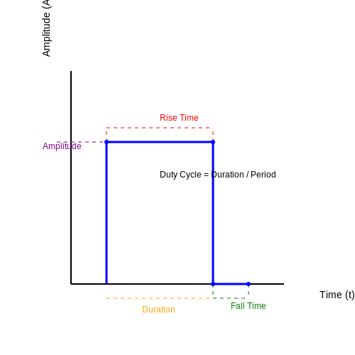
Duration: This is the total time the pulse remains at a high or low state, typically measured in microseconds or nanoseconds.
Amplitude: The maximum value of the pulse, which determines its strength and effectiveness in communicating information.
Duty Cycle: The ratio of the time the pulse is at a high level to the total period of the waveform, expressed as a percentage. It indicates how long the signal is "on" versus "off."
Rise and Fall Time: The time taken for the signal to transition from a low to a high state (rise time) and from high to low (fall time).

Mathematical Representation of Pulse Waveforms

Mathematically, a rectangular pulse can be defined using the Heaviside step function, which allows for precise modeling of pulse characteristics. The pulse can be represented as follows:

$$ P(t) = A \cdot [H(t - t_{on}) - H(t - t_{off})] $$

In this equation:

P(t): The pulse waveform as a function of time.
A: Amplitude of the pulse.
H(t): The Heaviside function, defined as:

$$ H(t) = \begin{cases} 0 & \text{for } t < 0 \\ 1 & \text{for } t \geq 0 \end{cases} $$

t_on: The time at which the pulse begins.
t_off: The time at which the pulse ends.

This representation gives a clear understanding of how alters in time can shape a pulse waveform, making it relevant for both theoretical studies and practical applications in circuit design.

Types of Pulse Waveforms

Several fundamental types of pulse waveforms are prevalent in engineering practices:

Unipolar Pulses: These pulses extend above the zero-voltage level, typically measured as a positive voltage. They are simpler to generate; however, they may not effectively convey information over long distances due to their unidirectional nature.
Bipolar Pulses: Bipolar pulses alternate between positive and negative voltages. Often used in data transmission schemes, these pulses reduce the DC component and improve signal integrity over transmission lines.
Gaussian Pulses: Renowned for their smooth transition and minimal side lobes, Gaussian pulses find applications in communications and signal processing to minimize inter-symbol interference.
Monocycles: These represent short-duration pulses with a single peak, often used in ultra-wideband communications where bandwidth efficiency is paramount.

Applications of Pulse Waveforms

The versatile nature of pulse waveforms leads to their use in several advanced applications:

Data Communication: Pulse modulation techniques, such as Pulse Code Modulation (PCM), use discrete pulse signals to represent analog information, enabling efficient data transmission.
Radar Systems: In radar technology, pulse waveforms are used to determine the distance and velocity of objects based on the time it takes for a signal to reflect back.
Digital Circuits: Modern digital electronics utilize pulse waveforms for clock signals, which synchronize the operations of various circuit components, ensuring seamless data processing.

Understanding pulse waveforms enhances our ability to design and innovate technological solutions that require precision and reliability. Mastering their characteristics and applications is indispensable for engineers and researchers dedicated to advancing fields like telecommunications and electronic circuit design.

Diagram Description: A diagram would illustrate the key characteristics of pulse waveforms, such as duration, amplitude, rise and fall times, and duty cycle, visually representing their relationships and transitions over time.

3. Amplitude

3.1 Amplitude

In the realm of electrical waveforms, amplitude serves as one of the foundational parameters, quantifying the extent of signal variation. The amplitude reflects the maximum value of a waveform, fundamentally shaping its physical and perceptual characteristics. Observing waveforms through oscilloscopes or simulation software highlights this parameter’s significance not only in theoretical physics but also in practical applications like acoustics, telecommunications, and signal processing.

Understanding Amplitude in Context

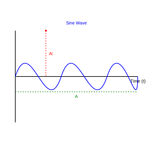
The term amplitude can broadly apply to various types of waveforms, including sinusoidal, square, triangular, or complex wave shapes. While the mathematical definition provides an abstraction, amplitude is directly observable in physical phenomena, such as the height of ocean waves or the intensity of sound waves. In the case of a sinusoidal waveform, mathematical representation is concise:

$$ A(t) = A_0 \sin(\omega t + \phi) $$

Here, A represents the instantaneous amplitude, A₀ the peak amplitude, ω the angular frequency, t time, and φ the phase shift. It’s crucial to differentiate peak amplitude, A₀, from root mean square (RMS) amplitude, which is often more representative of how energy is distributed in the waveform.

Mathematical Derivation of RMS Amplitude

RMS amplitude is a pertinent concept in real-world applications, especially in AC circuit calculations where effective voltage or current matters. The RMS value for a continuous function over one period (T) is calculated as follows:

$$ A_{RMS} = \sqrt{\frac{1}{T} \int_0^T A(t)^2 \, dt} $$

For a pure sinusoidal waveform, where A(t) = A_0 \sin(\omega t), substituting in gives:

$$ A_{RMS} = \sqrt{\frac{1}{T} \int_0^T (A_0 \sin(\omega t))^2 \, dt} $$

The integration bounds over one full cycle (consider ω = 2π/T) allows us to evaluate the integral. The solution simplifies to:

$$ A_{RMS} = \frac{A_0}{\sqrt{2}} $$

This factor underscores why RMS amplitude plays a crucial role in power calculations across AC circuits, as it correlates directly with the effective power delivered to resistive loads.

Practical Relevance and Applications

Amplitude is not merely a theoretical concept; it translates directly into the performance of devices and systems across disciplines:

Telecommunication: Signal amplitude defines the strength of a transmitted signal, impacting clarity and range.
Audio Engineering: Amplitude controls the loudness of audio signals, fundamentally affecting user experience.
Medical Imaging: In technologies such as ultrasound, amplitude variations signify different tissue densities, critical for diagnostic purposes.

Thus, understanding amplitude is essential for engineers and researchers working to optimize performance in these fields. The manipulation of amplitude through gain control, filtering, and modulation techniques are core to enhancing signal fidelity and reliability, ensuring effective communication, whether through sound or electromagnetic signals.

Diagram Description: The diagram would illustrate the sinusoidal waveform's amplitude, showing peak amplitude and RMS amplitude visually, allowing for immediate comparison of these two values within the context of the waveform.

3.2 Frequency

In the realm of electrical waveforms, frequency is a fundamental parameter that characterizes the oscillations of signals. It is defined as the number of complete cycles of a periodic waveform that occur in one second, with units measured in Hertz (Hz). Understanding frequency is crucial not only for theoretical physics but also for practical applications in engineering, telecommunications, audio technologies, and beyond.

Nature of Frequency

The concept of frequency extends beyond simple oscillations; it embodies the behavior of various physical systems. A deeper examination reveals that frequency can influence many properties of waveforms including amplitude, phase, and shape. For instance, in sound waves, higher frequencies correspond to higher pitches, while in electromagnetic waves, different frequencies denote different types of radiation, such as radio waves or X-rays. Mathematically, the frequency $ f $ of a waveform is related to the period $ T $, which is the duration of one cycle. This relationship is expressed as:

$$ f = \frac{1}{T} $$

Here, $ f $ is in Hertz (Hz) and $ T $ is in seconds. The reciprocal relationship between frequency and period is fundamental, indicating that as frequency increases, the duration of each cycle decreases.

Waveform Analysis and Frequency Components

When analyzing complex waveforms, Fourier analysis becomes an invaluable tool. According to the Fourier theorem, any periodic waveform can be decomposed into a sum of sine and cosine functions, each corresponding to different frequencies. This decomposition is expressed as:

$$ f(t) = \sum_{n=0}^{\infty} (A_n \cos(2 \pi n f_0 t) + B_n \sin(2 \pi n f_0 t)) $$

In this equation, $ A_n $ and $ B_n $ are the Fourier coefficients that determine the amplitude of each harmonic component, and $ f_0 $ is the fundamental frequency of the waveform. The practical implications of this decomposition are vast; for example, in signal processing, filters can be designed to allow only certain frequencies to pass, effectively manipulating the waveform for desired outcomes.

Real-World Frequency Applications

Frequency impacts a multitude of fields, such as:

Communications Technology: In radio transmission, different frequencies are used for various services (AM, FM, TV), which enables multiple stations to coexist while transmitting different information.
Audio Engineering: Sound designers utilize frequency manipulation to achieve various auditory effects. Equalizers, for instance, adjust the amplitude of specific frequency ranges, enhancing or diminishing sound quality.
Medical Imaging: Techniques like MRI rely on the concept of resonance at specific frequencies to generate images of the human body.

Conclusion

A profound understanding of frequency and its implications on waveforms is vital for both academic research and various engineering applications. The flexibility to manipulate frequency components in electrical signals empowers innovators to create new technologies and improve existing ones, illustrating the importance of this concept across multiple domains in science and technology. Each application opens doors to further research, driving progress in fields reliant on the precision and analysis of electrical waveforms.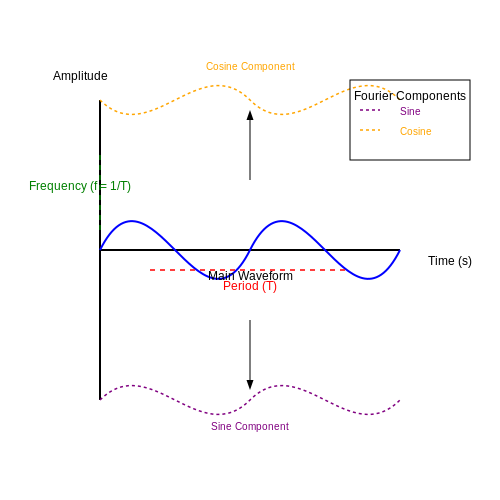

Diagram Description: A diagram would show the relationship between frequency and period visually, illustrating how an increase in frequency results in a decrease in the time duration of each cycle. Additionally, including a representation of Fourier analysis would depict how complex waveforms can be decomposed into their harmonic frequency components.

3.3 Period

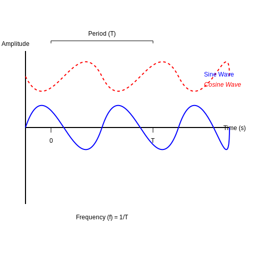
The concept of period is central to understanding electrical waveforms, particularly in the context of periodic signals. The period of a waveform is defined as the smallest interval over which the waveform repeats itself. This fundamental property not only embodies the behavior of the waveform but also has significant implications in both theoretical and practical aspects of electrical engineering and physics.

Understanding Period in Waveforms

Mathematically, the period $T$ of a waveform is the reciprocal of its frequency $f$. This relationship can be expressed with the equation:

$$ T = \frac{1}{f} $$

Here, the frequency $f$ is measured in Hertz (Hz), which denotes cycles per second. For instance, a signal with a frequency of 60 Hz will have a period of:

$$ T = \frac{1}{60} \approx 0.01667 \text{ seconds} $$

This means that the waveform completes one full cycle every 0.01667 seconds. Understanding this relationship is crucial when working with alternating current (AC) systems, where the frequency dictates the behaviour of electrical equipment such as transformers, motors, and even electronic circuits.

Practical Implications

The significance of the period extends beyond mere calculations; it plays a vital role in various applications:

AC Power Systems: In power distribution, the typical frequency is standardized (e.g., 50 Hz or 60 Hz), and understanding the period helps ensure devices are compatible with the electricity supply.
Signal Processing: In telecommunications and audio engineering, knowledge of the period ensures effective sampling rates, which is critical for accurate signal representation.
Control Systems: In feedback control systems, the period of input signals can significantly affect system stability and response times.

Comparison with Other Waveform Characteristics

The period is one of several key characteristics of waveforms. Others include:

Amplitude: The peak value of the waveform, which influences the power delivered by the signal and its effect on connected devices.
Phase: The position of the waveform relative to a time reference, which is crucial in applications involving multiple signals.
Shape: The form of the waveform—whether sinusoidal, square, triangular, etc.—affects how energy is transmitted through systems.

By comprehensively analyzing these characteristics in conjunction with the period, engineers and scientists can tailor systems for optimal performance in specific applications.

Conclusion

Understanding the concept of period in electrical waveforms is essential for professionals engaged in electronics, signal processing, and control systems. As a fundamental property, it links directly to the frequency and significantly impacts how electrical systems are designed and operated. Mastery of this concept allows engineers and researchers to innovate and improve upon existing technologies, ensuring robust and reliable electrical systems in the fast-evolving landscape of modern technology.

As you delve deeper into the study of electrical waveforms, consider how period interacts with other waveform characteristics to shape effective solutions in your projects and research endeavors.

Diagram Description: The diagram would illustrate the relationship between period and frequency in waveforms, visually representing how one waveform cycle relates to time and specifying the values of frequency and period for clarity. Additionally, it could show different waveform shapes to highlight how period varies across types.

3.4 Phase

In the study of electrical waveforms, the concept of phase plays a pivotal role in understanding how these waveforms interact with one another. Phase refers to a specific point in the cycle of a waveform, and it is typically measured in degrees or radians. The synchronization and timing of electrical signals are critical in various applications, including communications, signal processing, and power distribution. To grasp the notion of phase, it is essential to first understand the relationship between periodic waveforms. Consider two waveforms of the same frequency, $A$ and $B$. If these waveforms reach their maximum values simultaneously, they are said to be in phase. However, if one waveform reaches its maximum while the other is at zero, they are considered to be 90 degrees out of phase. The mathematical representation of the phase can be expressed as follows. For a sinusoidal waveform, we define the waveform $A(t)$ as: $$ A(t) = A_0 \sin(\omega t + \phi) $$ where: - $A_0$ is the amplitude, - $\omega$ is the angular frequency (related to the frequency $f$ by $\omega = 2\pi f$), - $t$ is time, - $\phi$ is the phase angle in radians. The phase angle $\phi$ is crucial as it dictates the waveform's initial position relative to a reference point. This becomes particularly important in systems where multiple waveforms interact. For instance, in alternating current (AC) circuits, the phase relationship between the voltage and current waveforms affects the real power delivered to the circuit, defined as: $$ P = VI \cos(\phi) $$ Here, $P$ represents the real power, $V$ is the instantaneous voltage, $I$ is the instantaneous current, and $\phi$ is the phase difference between them. To visualize the impact of phase difference, consider two sine waves. The first waveform, $A(t)$, may start at zero, while a second waveform, $B(t)$, might be shifted forward or backward in time. This phase shift can be represented as: $$ B(t) = A_0 \sin(\omega t + \phi + \Delta \phi) $$ where $\Delta \phi$ indicates the phase difference. As a practical application, phase detection methods are employed in various fields. For example, phase-locked loops (PLLs) are used in communication systems to synchronize signals. These systems continuously adjust a local oscillator's phase to match that of a reference signal, ensuring accurate data transmission and reduced errors. In the context of electronics, components like capacitors and inductors introduce phase shifts in AC circuits, making them essential for tuning and filtering applications. Understanding how these elements affect phase relationships is crucial for designing efficient circuits. The importance of phase extends into the realm of signal processing, where aligned or misaligned waveforms can determine the outcome of various algorithms and operations, such as in Fourier transform applications. To deepen your understanding, consider studying real-world cases of phase relationships in AC circuits and the implications they have on system performance, particularly in power electronics and telecommunications. Now that we have laid the groundwork for the concept of phase in electrical waveforms, we can further explore phase modulation techniques and their implications in communications systems. This exploration will unveil the intricate dance of synchronization and timing that defines modern electronics.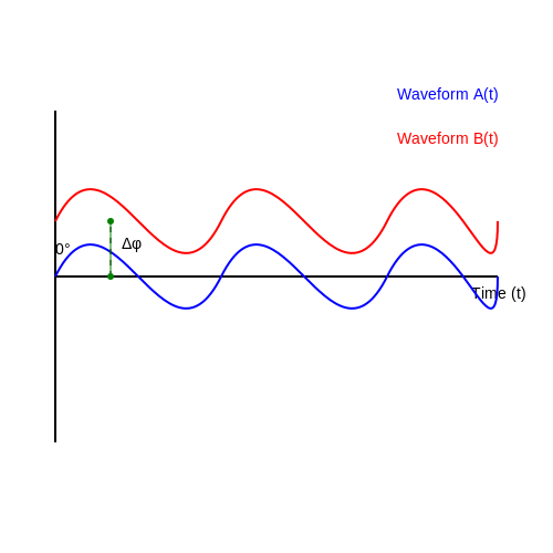

Diagram Description: The diagram would illustrate the phase relationship between two sine waveforms, showing their respective positions along the time axis and the resulting phase difference visually. This helps clarify how phase shifts affect synchronization in electrical signals.

3.5 Duty Cycle

The duty cycle is a critical concept in the analysis and design of electrical waveforms, especially in pulse width modulation (PWM) and signal processing applications. At its core, the duty cycle provides insight into the operational state of a signal, as it quantifies the proportion of time that a signal is in an active state compared to its total period. Understanding the duty cycle is key to optimizing circuit performance in various applications, including power supplies, motor control, and communication systems.

Definition and Basic Calculation

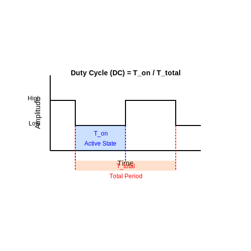
The duty cycle is defined mathematically as the ratio of the time the signal is high (active) to the total period of the waveform. It is usually expressed as a percentage. If we denote T_on as the time the signal is high and T_total as the total period of the waveform, the duty cycle (DC) can be expressed as:

$$ DC = \left(\frac{T_{on}}{T_{total}}\right) \times 100\% $$

For example, in a square wave where the signal is high for 2 ms and low for 3 ms, the total period T_total is 5 ms. Substituting these values into the formula gives:

$$ DC = \left(\frac{2\,\text{ms}}{5\,\text{ms}}\right) \times 100\% = 40\% $$

Applications of Duty Cycle

The varying duty cycles of signals enable numerous applications in electronics. One of the most notable areas is in PWM, where the duty cycle adjusts the average voltage delivered to an output load, such as a motor or LED. This allows for the effective control of power delivered without the need for bulky and inefficient analog components.

Motor Speed Control: By varying the duty cycle, an engineer can control the speed of a DC motor, allowing for precise adjustments in operations ranging from robotics to electric vehicles.
Brightness Control: Duty cycle modulation through PWM is widely used in LED lighting systems. By changing the duty cycle, the perceived brightness of an LED can be finely tuned, enhancing energy efficiency.
Signal Encoding: In communications, duty cycle manipulation can encode information, improving signal robustness against noise and interference.

Factors Influence Duty Cycle

Analyzing the duty cycle involves understanding how various factors—such as load characteristics, frequency, and control algorithms—can influence performance in real-world applications. For instance, high-frequency switching can lead to increased thermal loss in a device, necessitating careful duty cycle management to minimize power dissipation. Moreover, the operation of digital circuits often requires the synchronizing of duty cycles with system clocks to ensure signal integrity.

Conclusion

In summary, the duty cycle is a foundational element in understanding electrical waveforms, particularly in applications involving dynamic control and modulation of signals. Mastery of this concept enables engineers and researchers to design systems that are both efficient and effective in performance, paving the way for innovative solutions across multiple technologies.

Diagram Description: The diagram would physically show a waveform representing the duty cycle with clearly marked high and low periods, illustrating how the active time relates to the total period. It would also visually demonstrate the calculation of the duty cycle percentage.

4. Oscilloscope Overview

4.1 Oscilloscope Overview

In the realm of electrical engineering and experimental physics, the oscilloscope stands as an indispensable tool that visualizes electrical waveforms, allowing for detailed analysis of voltage, time, and transient phenomena. Understanding its functionalities not only enhances the ability to diagnose circuits but also enriches the grasp of signal behaviors in various applications ranging from simple electronics projects to advanced research endeavors.

What is an Oscilloscope?

An oscilloscope is an electronic instrument used to observe the changing signal voltages over time. It plots the output voltage on the vertical axis while time is represented on the horizontal axis. The resulting graph is known as a waveform, which provides insights into the signal's amplitude, frequency, and shape.

Key Components of an Oscilloscope

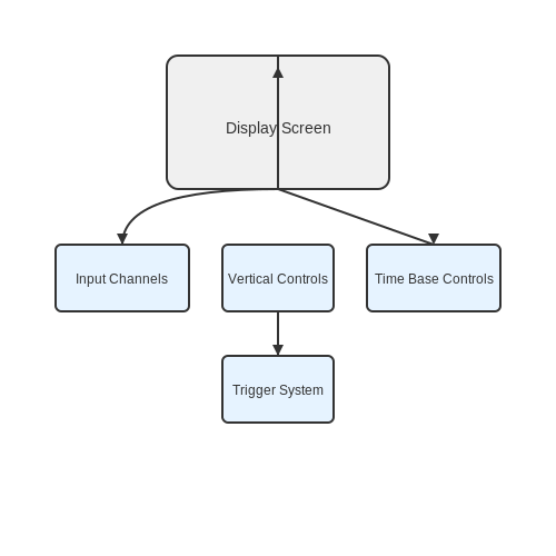
At its core, an oscilloscope comprises several critical components that work harmoniously to present accurate measurements. These include:

Display Screen: Visualizes the waveform in real-time.
Input Channels: Connects input signals from test points, often having multiple channels for comparative analysis.
Vertical Controls: Adjusts the scale of voltage on the display.
Time Base Controls: Configures the time scale to adapt the display to fast or slow signals.
Trigger System: Stabilizes repetitive waveforms ensuring that they are displayed consistently on the screen.

Types of Oscilloscopes

Oscilloscopes can be classified into different categories based on their technology and application. The main types include:

Analog Oscilloscopes: Utilize cathode ray tubes (CRTs) to display waveforms. Despite being less common in modern settings, they are prized for their simplicity and straightforward response.
Digital Oscilloscopes: Convert the input signal to digital format, enabling advanced features such as storage, signal processing, and complex triggering.
Mixed-Signal Oscilloscopes (MSOs): Combine the functionality of an analog oscilloscope and a logic analyzer, allowing engineers to observe both analog and digital signals simultaneously.

Practical Applications

The applications of oscilloscopes are vast and can be seen across numerous fields. In electronics, they are used for testing and troubleshooting circuits by observing signal shapes and timing relationships. In telecommunications, oscilloscopes analyze signal integrity, while in automotive technology, they help diagnose issues in electronic control units (ECUs). Furthermore, in physics research, oscilloscopes assist in studying wave phenomena and time-based experiments, making them crucial in both educational and professional laboratories.

Conclusion

The oscilloscope serves as a powerful window into the world of electrical signals. By mastering its functions and understanding its wave display capabilities, engineers and researchers can significantly enhance their ability to analyze and innovate within their fields. As technology advances, so too do the possibilities and features of oscilloscopes, continuing to push the boundaries of what can be understood through electrical waveforms.

Oscilloscope Overview in Electrical Waveforms

Diagram Description: The diagram would illustrate the key components of an oscilloscope, showing how each part interacts to display waveforms on the screen, which can be complex to visualize through text alone.

4.2 Using an Oscilloscope for Waveform Analysis

The oscilloscope serves as an indispensable tool in electrical engineering and experimental physics, offering a visual representation of electrical waveforms that can reveal crucial information about a circuit's behavior. Unlike multimeters, which provide only static measurements, oscilloscopes display waveforms in real time, enabling users to analyze dynamic changes in voltage and current over time.

Understanding the Basics of Oscilloscope Operation

To begin, an oscilloscope operates by sampling the voltage of an electrical signal and rendering it on a two-dimensional grid where the horizontal axis represents time and the vertical axis denotes voltage. The resulting display is a graphical representation of the waveform, which can exhibit various characteristics, such as amplitude, frequency, phase, and distortion. Understanding these characteristics is vital for accurate waveform analysis.

Typically, the oscilloscope captures the waveform using a probe connected to the circuit under investigation. The signal from the probe is fed into the input channels of the oscilloscope, which processes it and displays the resulting waveform. Different types of oscilloscopes are available, including analog and digital models, with digital oscilloscopes becoming more prevalent due to their advanced capabilities, such as storage and analysis.

Key Parameters to Measure

Amplitude: This indicates the maximum voltage level reached by the signal. It can provide insights into power levels and signals' strengths.
Frequency: The number of cycles per unit time, expressed in Hertz (Hz). This is a critical parameter for analyzing signal characteristics, particularly in communication and audio systems.
Phase Shift: The difference in phase between two signals can be observed to determine synchronization. This is especially crucial in applications involving multiple signals.
Rise and Fall Times: These metrics measure how quickly a signal transitions from low to high (and vice versa), revealing information about the bandwidth and speed of electronic components.

Calibration and Setup

Before initiating measurements, proper calibration of the oscilloscope is essential to ensure accuracy. This typically involves adjusting the vertical and horizontal scales according to the expected amplitude and frequency of the signal. Additionally, knowledge of the circuit’s characteristics will inform the choice of probes and their attenuation settings.

For accurate signal measurement, consider the following steps:

Connect the probe: Securely attach the probe tip to the point of interest in the circuit, ensuring that the ground clip is attached to the circuit ground.
Select the channel: Choose the appropriate channel on the oscilloscope for your measurement, adjusting the settings as needed.
Adjust the oscilloscope settings: Modify the time base and voltage scales to clearly observe the waveform. Utilize triggering options to stabilize the display.

Analyzing Waveform Data

Once the waveform is displayed, it is crucial to engage in a methodical analysis. Oscilloscopes often come equipped with built-in measurement tools that allow for automatic readings of amplitude, frequency, and other key parameters. However, manual measurements may be necessary in certain cases for a more in-depth understanding.

For practical applications, consider the following analysis techniques:

FFT Analysis: Many digital oscilloscopes provide a Fast Fourier Transform (FFT) function, which allows for spectral analysis. This can be invaluable in identifying signal harmonics and noise in complex signals.
Persistence Mode: This feature enables the oscilloscope to store and display multiple cycles of a waveform. This is beneficial when observing transient signals or infrequent events.
Triggering Options: Adjusting the triggering settings is crucial for capturing specific events within a signal and reducing noise.

In summary, the utilization of oscilloscopes in waveform analysis equips engineers and researchers with the critical insights needed for designing, testing, and diagnosing electronic systems effectively. Mastery of these tools leads to enhanced capabilities in understanding dynamic electrical phenomena.

Using an Oscilloscope for Waveform Analysis in Electrical Waveforms

Diagram Description: The diagram would illustrate the oscilloscope's waveform display, showing the relationship between time (horizontal axis) and voltage (vertical axis), as well as key parameters like amplitude and frequency. This visual representation would clarify how oscilloscopes analyze electrical signals over time.

4.3 Signal Generators

In the realm of electrical engineering and signal processing, signal generators hold a paramount importance due to their ubiquitous applications in testing, research, and development. As we build upon our understanding of electrical waveforms, it becomes imperative to delve into the functionalities and types of signal generators, their operational principles, and their practical implications in real-world scenarios. Signal generators can be classified into various categories based on their output characteristics, including function generators, signal sources, and sweep generators. Each type possesses unique attributes that cater to different applications, thus providing versatility in experimental setups and design validation.

Understanding Signal Generators

Signal generators are electronic devices that produce electronic signals with specified properties such as frequency, waveform, and amplitude. The ability to produce repetitive signals makes them essential tools in laboratories and field testing. The most commonly generated waveforms include:

Sine Waves: Generated using oscillators, ideal for applications requiring smooth harmonic signals.
Square Waves: Useful in digital circuits to represent binary signal states.
Triangular Waves: Employed in modulation and linear applications.
Sawtooth Waves: Often used in audio synthesizers for signal generation.

Each waveform carries distinct characteristics that influence the systems they interact with, making the choice of waveform critical depending on the testing or application requirements.

Operating Principles of Signal Generators

At the core of a signal generator lies an oscillator. An oscillator transforms direct current (DC) to alternating current (AC), generating the desired signal type. For instance, in a typical sine wave generator, a feedback loop utilizing an operational amplifier amplifies and filters the output to achieve the waveform's smoothness and frequency stability. The mathematical representation of these waveforms can be described using trigonometric functions. For example, a sine wave can be expressed as:

$$ V(t) = V_m \sin(2\pi ft + \phi) $$

Where: - $ V(t) $ is the instantaneous voltage, - $ V_m $ is the amplitude, - $ f $ is the frequency, - $ \phi $ is the phase shift. This equation encapsulates the essence of periodic signals and provides a foundation for understanding how variations in frequency and amplitude affect the output in practical applications.

Applications of Signal Generators

The applications of signal generators span across various fields, including: - Testing Electronic Devices: Signal generators create reference signals that are utilized to test various equipment, ensuring their functionality under different conditions. - Communications Systems: They generate modulated signals for transmitting data over communication channels, proving essential in both analog and digital formats. - Sensor Simulation: In system development, signal generators can be used to simulate sensor outputs, allowing for testing and calibration of signal processing circuits without the need for physical sensors. - Research and Development: Within the domains of physics and engineering, signal generators serve as critical tools for experimental setups, enabling researchers to explore the interplay of circuits and feedback mechanisms. Given this extensive applicability, understanding the operational theory behind signal generators is fundamental for engineers and researchers aiming to innovate and solve complex challenges in electronics. In conclusion, signal generators serve as the backbone of waveform production within the domain of electrical engineering. Their diverse functionalities and applications equip professionals with the tools necessary to validate designs and support advances in technology. Through the mastery of these devices and their characteristics, one can significantly enhance their effectiveness in both research and practical scenarios.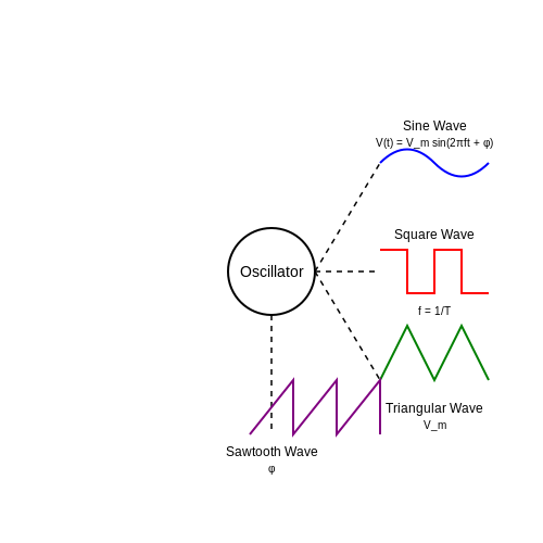

Signal Generators in Electrical Waveforms

Diagram Description: The diagram would illustrate the different types of waveforms generated by signal generators, as well as showcase the operational principles behind an oscillator transforming DC to AC. This visual representation would clarify how waveforms like sine, square, and triangular are produced and their relationships.

5. Communication Systems

5.1 Communication Systems

One of the most significant applications of electrical waveforms arises within the field of communication systems. Here, the transformation of information into electrical signals enables the efficient transmission of data over various media. As we delve into this domain, we will explore the nature of waveforms, modulation techniques, and their impact on modern communication technologies.

Understanding Waveforms in Communication

In communication systems, waveforms represent the state of an electrical signal as a function of time. They can be analog, such as sine waves, or digital, like square waves. The primary goal is to convey information by modulating these waveforms—altering certain attributes—such as amplitude, frequency, or phase. Consider the concept of amplitude modulation (AM), where information is encoded by varying the amplitude of a carrier wave. This contrasts with frequency modulation (FM), which encodes information by altering the carrier wave's frequency. The modulation scheme chosen determines the signal's resilience to noise, its bandwidth requirements, and the overall quality of the transmission.

The Role of Bandwidth

When discussing waveform processing in communication systems, the concept of bandwidth is critical. Bandwidth refers to the range of frequencies over which a waveform can operate effectively without degrading its performance. All communication mediums, whether wired or wireless, have inherent bandwidth limitations. For a more quantitative perspective, let us consider the Nyquist theorem, which provides insight into the maximum data rate, $ C $, that can be achieved over a band-limited channel:

$$ C = 2B \log_2(M) $$

In this formula: - $ C $ is the channel capacity in bits per second (bps). - $ B $ is the bandwidth of the channel in hertz (Hz). - $ M $ represents the number of discrete signal levels. A real-world application of this theorem can be seen in the design of both wired (e.g., DSL) and wireless (e.g., Wi-Fi) communication systems.

Modulation Techniques

Different modulation techniques serve various scenarios and requirements. Let's briefly discuss some common ones:

Amplitude Modulation (AM): Varies the amplitude of the carrier wave, primarily used in radio broadcasting.
Frequency Modulation (FM): Changes the frequency of the carrier wave; notably used in audio transmissions for better sound quality than AM.
Phase Modulation (PM): Alters the phase of the carrier wave, used in digital signal processing.
Quadrature Amplitude Modulation (QAM): Combines amplitude and phase modulation, commonly utilized in television broadcasting and broadband communications.

Each modulation technique has its strengths and weaknesses in terms of complexity, power efficiency, and resilience to interference.

Real-World Applications

Today, communication systems are embedded in our daily lives, from mobile devices to satellite communications. The selection of appropriate waveforms and modulation techniques directly impacts the performance of these systems. For example, in mobile communication, different modulation schemes adapt to various user requirements and environments. 4G and 5G networks leverage advanced QAM and OFDM (Orthogonal Frequency Division Multiplexing) to achieve high data rates and low latency, enabling seamless streaming, gaming, and data-intensive applications. As we advance further into the realm of communication technologies, the concepts of waveforms and modulation will continually evolve, addressing the increasing demand for speed, bandwidth, and reliability in data communication.

Conclusion

Understanding waveforms within communication systems is fundamental for any engineer or researcher in the field. By mastering modulation techniques and the role of bandwidth, one can effectively design systems that meet the communication demands of tomorrow.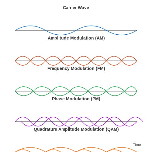

Communication Systems in Electrical Waveforms

Diagram Description: A diagram would visually illustrate the various modulation techniques (AM, FM, PM, QAM) by showing their waveforms and how they differ in amplitude, frequency, and phase. This visualization would enhance understanding of their respective characteristics and applications.

5.2 Power Electronics

Power electronics stands at the confluence of semiconductor technology and electromagnetic science, signaling a transformative approach to managing electrical energy. As various devices inherently operate using direct current (DC) or alternating current (AC), power electronics enables effective transition and control of these forms of electrical energy, crucial for modern electrical systems. This intricate domain encompasses several key components, circuits, and methodologies that allow for an array of applications, from renewable energy systems to efficient electric drive technology.

Fundamental Concepts in Power Electronics

To grasp the operational principles underlying power electronics, it is essential to be familiar with certain key concepts.

Switching Devices: At the heart of power electronic systems are switching devices such as diodes, transistors (BJT, MOSFET, IGBT), and thyristors. These components enable the control of power delivery to loads through rapid switching, which can maximize efficiency by minimizing energy loss.
Conversion Techniques: Power electronics primarily deals with the conversion of electrical energy between various forms and voltages. This includes AC to DC conversion (rectification), DC to AC conversion (inversion), and AC to AC or DC to DC conversions, depending on the configuration of the circuits and desired output.
Control Strategies: Effective control strategies are significant in addressing issues such as voltage regulation, harmonic mitigation, and transient response. Techniques like Pulse Width Modulation (PWM) have emerged as a cornerstone for efficiently managing the energy flow in these systems.

Mathematical Foundation

The principles governing power electronics can be elucidated through key equations that describe the relationships between voltage, current, and power. For instance, one of the fundamental relationships that must be understood is the power equation itself.

$$ P = VI $$

Here, $ P $ represents the power in watts, $ V $ is the voltage in volts, and $ I $ is the current in amperes. In the context of AC systems, however, we must factor in the phase difference between voltage and current, represented by the power factor $ \cos(\theta) $:

$$ P_{avg} = VI \cos(\theta) $$

In practical scenarios where power conversion occurs, understanding the efficiency of these conversions can be expressed as:

$$ \eta = \frac{P_{out}}{P_{in}} \times 100\% $$

where $ \eta $ signifies the efficiency of the converter.

Applications of Power Electronics

The implications of power electronics are vast and varied. The following applications illustrate how power electronic devices and systems are pertinent to various sectors:

Renewable Energy Systems: In solar photovoltaic systems, power electronics enable the conversion of DC generated by solar panels into AC suitable for grid connection. This is achieved through inverters, which are a prime example of power electronic converters.
Electric Vehicles (EV): Power electronics facilitates the efficient operation of EV drive systems by converting battery DC into AC, enabling the drive motors' operation, and managing battery charging.
HVDC Transmission: High Voltage Direct Current (HVDC) transmission systems leverage power electronics for efficient long-distance power transfer, minimizing line losses that occur over extended transmission lines.

Through the integration of power electronics into these applications, engineers can achieve enhanced efficiency, performance, and reliability, significantly impacting the overall economy of energy use.

Closing Thoughts

The realm of power electronics is continuously evolving, enriched by advancements in semiconductor materials, control algorithms, and integration techniques. As electric energy demand intensifies globally, the proficiency in designing and optimizing power electronic systems will remain a crucial skill for future engineers and technologists. Understanding these principles and applications provides a solid foundation for further exploration in this significant domain.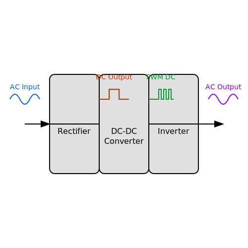

Power Electronics in Electrical Waveforms

Diagram Description: The diagram would illustrate the various types of power electronic converters (like rectifiers, inverters, and DC-DC converters) along with their input and output waveforms, showing how electricity transforms between different forms. This visual representation would clarify complex conversion techniques that involve both AC and DC systems.

5.3 Signal Processing

Signal processing is a critical component in the field of electrical engineering and physics, particularly when dealing with electrical waveforms, which are fundamental representations of electrical signals. The manipulation of these signals is essential for a variety of applications, spanning telecommunications, audio processing, image processing, and control systems. In this section, we will delve into various aspects of signal processing, examining essential concepts, techniques, and their practical applications.

Understanding Signal Processing

Signal processing involves the analysis, modification, and synthesis of signals. It employs mathematical techniques to process data measured over time or space, such as audio signals, sensor readings, and images. The fundamental goal is to improve the efficiency and performance of systems using these signals. There are two primary types of signal processing:

Analog Signal Processing — Operations performed on continuous-time signals.
Digital Signal Processing (DSP) — Techniques applied to discrete-time signals, typically implemented using algorithms on digital processors.

While both types have unique methodologies and applications, this section will primarily focus on digital signal processing, given its prevalence in modern technology.

The Mathematics of Signal Processing

At its core, digital signal processing operates on digital data representing continuous signals. The primary mathematical tools used in DSP are Fourier Transform and its variations, important for understanding signal frequency components. To convert a continuous-time signal, $ x(t) $, into a discrete-time signal, $ x[n] $, we sample the continuous signal at regular intervals governed by the sampling frequency, $ f_s $: $$ x[n] = x(nT) $$ where $ T $ is the sampling period (related to $ f_s $ by $ T = 1/f_s $). This transformation enables the use of digital techniques such as filtering, modulation, and spectral analysis. An essential aspect is the Nyquist-Shannon sampling theorem, which states that to avoid aliasing, the sampling frequency must be at least twice the highest frequency present in the signal: $$ f_s \geq 2f_{max} $$ In this case, $ f_{max} $ is the highest frequency contained in the original signal. With these concepts in hand, we can explore key techniques and applications in signal processing.

Key Techniques in Signal Processing

1. Filtering: Filtering techniques are essential for removing unwanted components from signals. Common types include: - Low-pass filters, which allow low-frequency signals to pass and attenuate high-frequency noise. - High-pass filters, which do the opposite, removing low-frequency trends and noise. - Band-pass filters, which permit signals within a specific frequency range to pass. 2. Fast Fourier Transform (FFT): The FFT is an algorithm to compute the Discrete Fourier Transform (DFT) efficiently. It provides frequency domain representations that are crucial for analyzing the spectral content of signals. 3. Wavelet Transform: Unlike the Fourier Transform, which provides a global analysis, the Wavelet Transform offers localized time-frequency analysis, making it suitable for processing transient signals. 4. Digital Modulation Techniques: These techniques such as Phase Shift Keying (PSK) and Frequency Shift Keying (FSK) are fundamental in digital communication systems to encode information onto a carrier wave.

Real-World Applications of Signal Processing

The applications of signal processing are vast and critical in various industries: - Telecommunications: Signal processing enhances communication quality by improving noise resilience and enabling data compression. - Audio Processing: Techniques in DSP have transformed music production, speech recognition, and noise cancellation technologies. - Medical Imaging: Imaging technologies like MRI and CT scans rely heavily on signal processing for image reconstruction and enhancement. - Control Systems: In automation and robotics, DSP techniques help in controlling dynamic systems through sensor data processing. Through the integration of these techniques, engineers can significantly enhance the performance of systems across disciplines. Signal processing, as explored here, is a powerful tool in the modern engineer's arsenal. It not only enhances our capability to manipulate and interpret data but directly impacts the efficiency and effectiveness with which we interact with the ever-evolving technological landscape. The knowledge of these principles constitutes a critical foundation for any advanced study or practical application in electronics and telecommunications.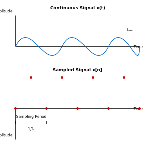

Signal Processing in Electrical Waveforms

Diagram Description: The diagram would illustrate the relationships between continuous-time signals, their discrete-time counterparts after sampling, and the Nyquist-Shannon theorem's implications on sampling frequency relative to the highest signal frequency.

6. Constructing a Simple Circuit with Waveforms

6.1 Constructing a Simple Circuit with Waveforms

In this subsection, we will delve into the practical construction of a basic circuit utilizing electrical waveforms. This subject is fundamental as it bridges the abstract concepts of waveforms with tangible physical applications, demonstrating how theoretical principles manifest in real circuits. By the end of this section, you will be equipped with knowledge about waveform generation, circuit assembly, and practical measurements.

Understanding Waveforms

Before constructing a circuit, it is critical to understand what waveforms represent. Waveforms are graphical representations of electrical signals that vary over time. They can take several forms such as sinusoidal, square, triangular, and sawtooth. Each waveform has distinct characteristics that influence how it interacts with circuit components. For instance, a sinusoidal waveform is characterized by its smooth periodic oscillations, often represented mathematically as:

$$ V(t) = V_{m} \sin(2\pi ft + \phi) $$

where $V_{m}$ is the peak voltage, $f$ is the frequency in hertz, and $\phi$ is the phase shift in radians. Understanding the parameters of waveforms is essential as they dictate the behavior of the circuit components such as resistors, capacitors, and inductors.

Components for the Circuit

To construct a simple circuit that generates and displays waveforms, you will need the following components:

Function Generator: This device generates various types of waveforms, essential for inputting the electrical signals into the circuit.
Oscilloscope: A crucial tool for visualizing waveforms, allowing you to observe and analyze signal changes over time.
Resistors, capacitors, and inductors: These components will be employed in various configurations to study how they respond to different waveforms.
Connecting wires and breadboard: For assembling the circuit in a flexible and experiment-friendly manner.

Constructing the Circuit

The next step involves assembling the circuit. We will create a simple RC (resistor-capacitor) low-pass filter circuit, which will allow sinusoidal waveforms to pass through while attenuating higher frequencies. Below are the steps to construct the circuit: 1. Set Up the Function Generator: Configure the function generator to produce a sinusoidal waveform at a desired frequency (e.g., 1 kHz) and amplitude (e.g., 5 V peak-to-peak). 2. Connect Circuit Components: Using connecting wires, connect the function generator's output to one terminal of the resistor. Connect the other terminal of the resistor to one terminal of the capacitor. Finally, ground the other terminal of the capacitor. 3. Connect Oscilloscope: Attach the probe of the oscilloscope to the junction between the resistor and capacitor to measure the voltage drop, which illustrates the filtered output waveform.

$$ f_c = \frac{1}{2\pi RC} $$

The cutoff frequency $ f_c $ represents the frequency above which the output signal starts to drop off and is determined by the values of the resistor $ R $ and capacitor $ C $.

Measurements and Observations

Once the circuit is assembled, observe the output waveform on the oscilloscope. Perform the following: 1. Adjust the frequency of the input waveform while monitoring the output on the oscilloscope. 2. Note how the amplitude and shape of the output waveform change as the input frequency approaches and surpasses the cutoff frequency ($f_c$). 3. Record your observations on how different values of $R$ and $C$ influence the circuit's response characteristics.

Practical Relevance and Applications

Understanding and constructing circuits with waveforms is vital in various applications. From filtering signals in communication systems to designing oscillators and amplifiers in audio engineering, the principles established here underpin much of modern electronics. This knowledge also serves as a foundation for more complex systems, such as converters and signal modulation techniques. In conclusion, by constructing this simple circuit, you will have hands-on experience with electrical waveforms and an appreciation for their fundamental role in the behavior of electronic systems. This practical understanding is essential for any advanced-level professional in the fields of physics and engineering.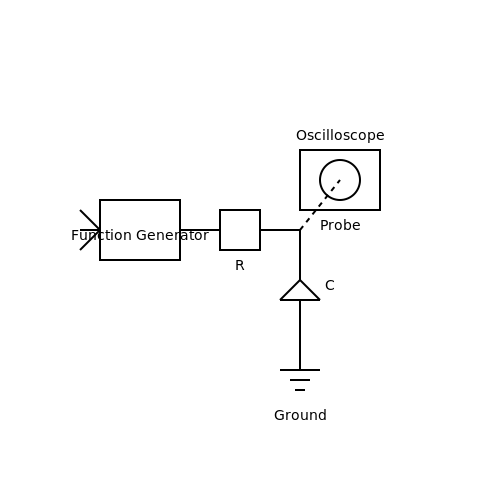

Constructing a Simple Circuit with Waveforms in Electrical Waveforms

Diagram Description: The diagram would visually depict the RC low-pass filter circuit layout, including the connections between the function generator, resistor, capacitor, and oscilloscope, clarifying signal flow and component interaction.

6.2 Measuring Waveform Characteristics

As we delve into the intricacies of electrical waveforms, an understanding of how to measure their characteristics becomes paramount. Waveforms are not just visual representations; they hold significant information about the underlying physics of electrical signals. This section explores how we quantitatively assess waveforms through several key characteristics, such as amplitude, frequency, phase, rise and fall times, and duty cycle.

Amplitude

Amplitude represents the maximum value of a waveform, whether it be voltage, current, or power. It is crucial for determining the signal strength and its effectiveness in communication systems. To measure the amplitude, one typically utilizes instruments like oscilloscopes or multimeters. Oscilloscopes allow for dynamic observation, capturing transient behaviors that might otherwise go unnoticed. Additionally, the peak-to-peak voltage (Vpp) is often calculated for periodic waveforms, defined mathematically as:

$$ V_{pp} = V_{max} - V_{min} $$

where $ V_{max} $ represents the maximum voltage, and $ V_{min} $ is the minimum voltage of the waveform.

Frequency

Frequency, the number of cycles of a waveform per second, is another critical characteristic, measured in hertz (Hz). It is crucial in applications such as communications, audio engineering, and signal processing. The frequency can be computed as the reciprocal of the period (T) of the waveform, expressed mathematically as:

$$ f = \frac{1}{T} $$

where: - $ f $ is the frequency, - $ T $ is the period, defined as the time taken for one complete cycle. Modern oscilloscopes can provide direct frequency readouts, aiding engineers and scientists in rapid assessments.

Phase

Phase differences between signals can significantly affect system performance, particularly in multi-signal environments. The phase of a waveform is typically measured in degrees. To analyze phase, one can compare the waveform of interest to a reference waveform. Mathematically, we express the phase difference ($ \phi $) as:

$$ \phi = \frac{360^\circ}{T} \cdot \Delta t $$

where $ \Delta t $ is the time difference between corresponding points of the two waveforms being compared. Oscilloscopes with cursor measurements or phase meters facilitate this analysis efficiently.

Rise and Fall Times

Rise time (tr) and fall time (tf) describe the transient response of a waveform, specifically the time taken for a signal to rise from 10% to 90% of its maximum value or fall from 90% to 10% of its maximum value, respectively. These parameters are crucial in characterizing high-speed digital signals. Mathematically, these times can be defined as:

$$ t_r = t_{90\%} - t_{10\%} $$

$$ t_f = t_{90\%} - t_{10\%} $$

The analysis of rise and fall times is vital for ensuring signal integrity in high-speed applications, affecting factors like data rates and system stability.

Duty Cycle

The duty cycle, defined as the ratio of the time a signal is active to the total period of the waveform, is usually expressed as a percentage. It plays a significant role in PWM (Pulse Width Modulation) applications. Mathematically, the duty cycle (D) can be expressed as:

$$ D = \left( \frac{T_{on}}{T_{on} + T_{off}} \right) \cdot 100 $$

where: - $ T_{on} $ is the time the signal is high, - $ T_{off} $ is the time the signal is low. A higher duty cycle indicates more power delivered to a load in pulse-width modulated systems, hence its crucial relevance in power electronics.

Conclusion and Practical Relevance

Understanding how to measure and interpret these characteristics of electrical waveforms is fundamental not only for academic pursuits but also for real-world applications in telecommunications, signal processing, and control systems. Engineers routinely assess these parameters to optimize system performance, ensuring effective communication and efficient power delivery in modern electronic devices. As we progress, exploring the tools and methodologies for these measurements will enrich our understanding of signal characteristics, equipping us for innovation in electronics and engineering. In the next section, we will explore the tools available for waveform analysis and their respective methodologies.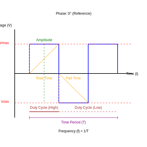

Measuring Waveform Characteristics in Electrical Waveforms

Diagram Description: A diagram would visually represent the amplitude, frequency, phase, rise and fall times, and duty cycle of waveforms, showing how these characteristics are measured and calculated. It would illustrate relationships that text alone cannot convey, particularly the time scale and signal levels.

6.3 Analyzing Circuit Behavior with Different Waveforms

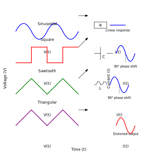
The behavior of electrical circuits is profoundly influenced by the type of waveform applied to them. In this section, we will explore how various waveforms—such as sinusoidal, square, sawtooth, and triangular—affect circuit performance. Each waveform produces different characteristics in circuit responses, allowing for a wide range of applications in electronics and signal processing.

An Overview of Waveforms

Electrical waveforms can be categorized based on their shape and characteristics:

Sinusoidal Waveforms: Represented by the function V(t) = V₀ sin(ωt + φ), where V₀ is the amplitude, ω is the angular frequency, and φ is the phase shift. Sinusoidal waveforms are fundamental in alternating current (AC) analysis.
Square Waveforms: Function as a series of abrupt transitions between high and low levels, often described as V(t) = V₀ sgn(sin(ωt)). They are extensively used in digital electronics.
Sawtooth and Triangular Waveforms: Typically used in signal generation, these waveforms offer linear ramp-up and ramp-down profiles.

Impact of Waveforms on Circuit Behavior

Understanding the impact of these waveforms on different types of circuits is crucial. Below, we will analyze how specific circuit components respond to these waveforms:

1. Resistor Circuits

In resistor circuits, the current follows Ohm's Law, regardless of the waveform applied. The relationship can be expressed as:

$$ I(t) = \frac{V(t)}{R} $$

This means that the current waveform will directly mimic the voltage waveform, scaled by the resistance. Such circuits are linear, exhibiting consistent behavior across all waveform shapes.

2. Capacitor Circuits

Capacitors introduce phase shifts between voltage and current. For a sinusoidal input, the relationship can be derived from:

$$ V_C(t) = \frac{1}{C} \int I(t) dt $$

Thus, the current leads the voltage by 90 degrees. In the case of a square or triangular waveform, the capacitor will charge and discharge differently, resulting in various current waveforms and possibly significant distortion.

3. Inductor Circuits

Inductors, on the other hand, oppose changes in current. With a sinusoidal voltage:

$$ V_L(t) = L \frac{dI(t)}{dt} $$

The voltage across the inductor will lead current by 90 degrees. Non-sinusoidal inputs will lead to complex interactions, including harmonic distortion, especially evident with square waves.

Practical Applications

The analysis of circuit behavior under different waveforms has practical significance in various fields:

Signal Processing: Different waveforms are used for modulation in communication systems where bandwidth and distortion considerations are critical.
Power Electronics: Understanding waveform distortion and harmonics is essential for designing filters and converters.
Testing and Measurement: Testing devices often need to evaluate circuit response to different waveforms to ascertain reliability and performance.

In summary, analyzing circuit behavior with various waveforms allows engineers to develop better designs for specific applications, ensuring efficient operation and enhanced performance across a multitude of electronic systems.

Analyzing Circuit Behavior with Different Waveforms in Electrical Waveforms

Diagram Description: The diagram would illustrate the various voltage waveforms (sinusoidal, square, sawtooth, and triangular) along with their transformations across different circuit components (resistor, capacitor, inductor), showing phase shifts and waveform interactions visually.

7. Recommended Textbooks

7.1 Recommended Textbooks

Electric Circuits by James W. Nilsson and Susan Riedel — This textbook covers fundamental electrical engineering concepts and introduces electrical waveforms with detailed examples and problem-solving techniques. It's particularly suited for advanced undergraduate and graduate students.
RF and Microwave Circuit Design by Charles E. Free — This book provides an in-depth look into microwave circuit design and includes real-world applications of waveform analysis in high-frequency circuits, which is essential for understanding modern communication systems.
Signals, Systems, and Transforms by Charles L. Phillips and John Parr — An excellent resource for comprehending the mathematical methods behind waveforms. The book balances theory with practical insights into transforms, signals processing, and real-world waveform applications.
Electronics and Circuit Analysis using MATLAB by John Okyere Attia — A hands-on guide for circuit analysis using MATLAB, focusing on waveform generation and visualization, ideal for researchers interested in practical computational tools for electrical engineering.
Principles of Modern Radar: Basic Principles — Offers essential insights into radar systems where waveform analysis plays a critical role. Useful for professionals dealing with radar systems and looking for a comprehensive overview of radar waveform properties.
Fundamentals of Electric Power Quality by Surya Santoso — This book addresses waveform quality in power systems, including harmonic distortion analysis crucial for ensuring optimal power delivery and system reliability.
Modern Digital and Analog Communication Systems by B.P. Lathi and Zhi Ding — A detailed exploration of both digital and analog communication techniques with comprehensive sections on waveform analysis, modulation, and noise in communication circuits.

7.2 Online Resources

Electronics Tutorials — This website offers a comprehensive set of tutorials on electrical waveforms and circuits. It includes detailed explanations, diagrams, and practical examples relevant to engineers and advanced students.
WikiElectronics — A collaborative platform providing in-depth articles on various electronic concepts, including detailed guidance on understanding and utilizing electrical waveforms in real-world applications.
Khan Academy Electrical Engineering — Offers a series of lectures and notes on foundational and advanced concepts in electrical waveforms as part of its engineering courses.
National Nanotechnology Initiative — While this source focuses broader on matter at the nanoscale, it also provides relevant articles on electrical waveforms and nanoelectronics, connecting micro-scale electrical phenomena to practical scenarios.
Coursera - Electrical Engineering Course — An online course that spurs a deeper understanding of electrical waveform generation, manipulation, and application, complete with video lectures, readings, and quizzes.
EdX - Electronics by The University of California, Berkeley — Provides a rigorous, university-level study on electronics and waveform analysis. Ideal for self-paced learners interested in comprehensive learning.
Understanding Electrical Waveforms - ECM — A practical guide that explains electrical waveforms through a series of industry-relevant applications and videos, suitable for professionals and researchers looking for applied knowledge.

7.3 Research Papers

Waveform Analysis of Electrical Circuits — This paper provides an in-depth study on various waveform behaviors in electrical circuits. It reviews both theoretical and practical aspects and offers experimental data to validate the theoretical assumptions.
Nonlinear Dynamics of Electrical Waveforms — Explores the nonlinear phenomena in electrical waveforms. This research emphasizes understanding the impact of nonlinearity on circuit performance, essential for advanced electronic designs.
Physics Reports on Signal Processing via Electrical Waveform Analysis — A comprehensive report discussing the methods of signal processing and system identification through waveform analysis, detailing various algorithmic approaches.
Advanced Measurement Techniques for Electrical Waveforms — Focuses on state-of-the-art methods for measuring complex waveforms. It offers insights into the latest technological advancements and their implementation in modern electronic applications.
Critical Analysis of Waveform Dynamics in Electric Systems — Analyzes critical aspects of waveform behaviors and dynamics in electrical systems, offering an analysis framework useful for researchers involved in power electronics and circuit design.
Real-world Applications of Electrical Waveforms in Engineering — Discusses the practical applications of waveform analysis in engineering, highlighting how theoretical concepts translate into real-world challenges and solutions.
Optoelectronic Conversion of Electrical Waveforms — Investigates the optoelectronic conversion processes used in modern applications, including challenges and innovations in converting and managing electrical waveforms.