Fairness Evaluation Metrics for ML Models
1. Definition and Importance of Fairness
Definition and Importance of Fairness
Fairness in machine learning refers to the absence of bias or discrimination in algorithmic decision-making against individuals or groups based on protected attributes such as race, gender, age, or socioeconomic status. Formally, fairness can be expressed through statistical parity, where the probability of a favorable outcome is equal across different groups:
where Ŷ represents the model's prediction, and A denotes the protected attribute with values a and b for different groups. This condition, known as demographic parity, ensures equal acceptance rates across groups but may conflict with other fairness criteria like equalized odds or predictive parity.
Why Fairness Matters
The importance of fairness stems from both ethical and practical considerations:
- Ethical obligations: ML models increasingly influence high-stakes domains like hiring, lending, and criminal justice. Biased decisions can perpetuate historical inequalities.
- Legal compliance: Many jurisdictions enforce anti-discrimination laws (e.g., EU's GDPR, US Civil Rights Act) that apply to algorithmic systems.
- Model performance: Unfair models often exhibit poorer generalization across subgroups, leading to degraded performance on underrepresented populations.
- Reputational risk: Publicized cases of algorithmic bias (e.g., COMPAS recidivism tool, gender-biased hiring algorithms) have led to significant backlash against organizations.
Key Fairness Concepts
Fairness definitions can be categorized based on their mathematical formulation:
Group Fairness
Measures disparities in outcomes between protected groups. Common metrics include:
A value less than 0.8 (the "80% rule") may indicate discrimination under US employment law.
Individual Fairness
Requires that similar individuals receive similar predictions, formalized as:
where D measures prediction distance and d measures input similarity.
Trade-offs in Fairness
Several impossibility results demonstrate inherent tensions between fairness criteria:
- Except in trivial cases, no classifier can simultaneously satisfy calibration and equalized odds (Kleinberg et al., 2016).
- Perfect predictive parity often requires different decision thresholds for different groups, potentially violating anti-discrimination laws.
These trade-offs necessitate careful consideration of which fairness criteria align with the specific application context and ethical priorities.
1.2 Common Biases in ML Models
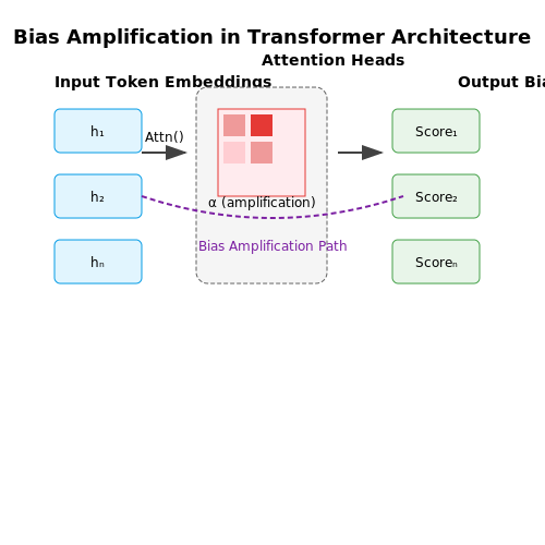
Machine learning models often inherit or amplify biases present in training data, leading to unfair outcomes across demographic groups. These biases manifest in various forms, each with distinct mathematical and operational characteristics.
Statistical Bias
Statistical bias occurs when a model systematically underestimates or overestimates a parameter due to flawed assumptions in the learning algorithm. For a model parameter θ̂ estimating true parameter θ, the bias is defined as:
In practice, this emerges when features correlated with protected attributes (e.g., race or gender) disproportionately influence predictions. For example, a hiring model trained on historical data may inherit gender disparities if past hiring patterns were biased.
Representation Bias
This arises when training data underrepresents certain groups. Consider a facial recognition system trained primarily on lighter-skinned individuals. The model's error rate ϵ for underrepresented group g will satisfy:
where ng is the sample size for group g. The 2018 Gender Shades study demonstrated commercial systems had up to 34.7% higher error rates for darker-skinned females compared to lighter-skinned males.
Measurement Bias
Occurs when feature measurement processes systematically distort reality. In credit scoring, ZIP code-based features may proxy for race due to historical redlining. The bias propagates through the model as:
where Δ represents the measurement distortion correlated with protected attributes.
Aggregation Bias
Happens when models assume uniform relationships across groups despite heterogeneous patterns. A single model trained on aggregated data may perform poorly for subgroups where:
for subgroups z1 and z2. This was observed in healthcare risk prediction models that underestimated needs for Black patients by using cost as a proxy for health status.
Evaluation Bias
Occurs when performance metrics fail to account for subgroup disparities. A model achieving 90% overall accuracy might have:
The COMPAS recidivism algorithm exhibited this pattern, with higher false positive rates for Black defendants despite comparable overall precision.
Temporal Bias
Emerges when models trained on historical data fail to adapt to changing social norms. The bias compounds over time t as:
where λ represents the rate of societal change. This was observed in resume screening tools that penalized women's resumes for career gaps, despite evolving workplace norms.
1.3 Legal and Ethical Considerations
Machine learning models deployed in high-stakes domains such as hiring, lending, and criminal justice must comply with legal frameworks designed to prevent discrimination. Key regulations include the General Data Protection Regulation (GDPR) in the EU, which mandates algorithmic transparency (Article 22), and the U.S. Equal Credit Opportunity Act (ECOA), prohibiting credit discrimination based on protected attributes like race or gender. Violations can result in legal penalties, reputational damage, and loss of public trust.
Legal Frameworks Governing Fairness
GDPR’s right to explanation requires that individuals subject to automated decision-making receive meaningful information about the logic involved. This intersects with fairness metrics when models use proxies for protected attributes. For example, a hiring model trained on historical data may inadvertently encode gender bias through correlated features like "college major." The U.S. Civil Rights Act (Title VII) further prohibits disparate impact, where neutral policies disproportionately harm protected groups. Courts apply the 80% rule (EEOC, 1978): if the selection rate for a protected group is less than 80% of the highest rate, discrimination is presumed.
Ethical Tensions in Fairness Metrics
Legal compliance does not guarantee ethical fairness. Tensions arise between:
- Individual vs. Group Fairness: Satisfying statistical parity (group fairness) may require violating consistency (individual fairness), where similar individuals receive divergent outcomes.
- Accuracy-Fairness Tradeoffs: Constraining models to meet fairness criteria (e.g., demographic parity) often reduces accuracy. The impossibility theorem (Kleinberg et al., 2017) proves that no model can simultaneously satisfy calibration, balance, and independence.
Case Study: COMPAS Recidivism Algorithm
ProPublica’s 2016 analysis revealed that the COMPAS tool falsely flagged Black defendants as high-risk at twice the rate of White defendants, violating error rate balance. While the tool satisfied predictive parity (equal precision across groups), this case highlighted the inadequacy of single-metric fairness evaluations and spurred debates on metric selection in legal contexts.
Mitigation Strategies
Organizations should:
- Conduct disparate impact analyses during model development, using metrics like standardized mean difference (SMD) for continuous outcomes:
- Implement regular audits with tools like IBM’s AI Fairness 360 or Google’s What-If Tool to monitor post-deployment drift in fairness metrics.
- Establish redress mechanisms for affected individuals, aligning with GDPR’s Article 35 requirements for human oversight of automated systems.
2. Demographic Parity
Demographic Parity
Demographic parity, also known as statistical parity, is a fairness criterion that requires a machine learning model's predictions to be statistically independent of protected attributes such as race, gender, or age. Formally, a binary classifier satisfies demographic parity if the probability of a positive outcome is equal across all demographic groups. This ensures that no group is disproportionately advantaged or disadvantaged by the model's decisions.
Mathematical Definition
Let Ŷ denote the model's prediction (binary outcome) and A represent the protected attribute (e.g., gender with values a₁, a₂, ..., aₖ). Demographic parity is satisfied if:
In simpler terms, the likelihood of receiving a favorable prediction should not vary based on group membership. For example, if A represents gender, the proportion of loan approvals (Ŷ = 1) should be identical for male and female applicants.
Measuring Demographic Parity
The disparity in positive prediction rates across groups can be quantified using the demographic parity difference (DPD):
A model achieves perfect demographic parity if DPD = 0. In practice, a small non-zero threshold (e.g., DPD ≤ 0.05) is often tolerated.
Limitations and Trade-offs
While demographic parity enforces equal outcomes, it does not account for differences in underlying group distributions or legitimate factors influencing the prediction. For instance, if one demographic group genuinely qualifies for loans at a higher rate, enforcing strict parity may require artificially lowering approval rates for that group, leading to reverse discrimination.
Additionally, demographic parity ignores base rate disparities—differences in the true prevalence of the outcome (Y) across groups. If P(Y = 1) varies by group, enforcing equal P(Ŷ = 1) may result in higher error rates for some groups.
Practical Implementation
To enforce demographic parity during model training, techniques such as:
- Pre-processing: Adjust training data to balance group representation (e.g., reweighting or resampling).
- In-processing: Incorporate fairness constraints into the optimization objective (e.g., adversarial debiasing).
- Post-processing: Modify model outputs to equalize prediction rates (e.g., threshold adjustment per group).
For example, in a hiring model, post-processing might involve setting group-specific decision thresholds to ensure equal selection rates.
Case Study: Credit Scoring
A 2019 study by Hardt et al. evaluated demographic parity in credit scoring models. The researchers found that enforcing strict parity reduced disparities in approval rates but increased false negatives for historically disadvantaged groups. This highlights the trade-off between fairness and accuracy when using demographic parity as a constraint.
2.2 Equalized Odds
Equalized Odds is a fairness criterion that requires a classifier's predictions to be conditionally independent of the sensitive attribute given the true label. Formally, for a binary classifier h, sensitive attribute A, and true label Y, the condition is satisfied when:
for all values of a and y. This implies that the true positive rate (TPR) and false positive rate (FPR) must be equal across all groups defined by A.
Mathematical Derivation
Let TPRa and FPRa denote the true positive rate and false positive rate for group a, respectively. Equalized Odds requires:
These constraints can be expressed in terms of the confusion matrix. For a binary classifier, the confusion matrix for group a is:
where TNa, FPa, FNa, and TPa are the counts of true negatives, false positives, false negatives, and true positives, respectively. The TPR and FPR for group a are then:
Equalized Odds holds when these rates are equal across all groups.
Practical Implications
Enforcing Equalized Odds often involves trade-offs with overall model accuracy. For instance, a classifier optimized purely for accuracy may achieve higher performance by exploiting correlations between the sensitive attribute and the target label, violating Equalized Odds. Techniques to satisfy this criterion include:
- Post-processing: Adjusting decision thresholds for different groups to equalize TPR and FPR.
- Constrained optimization: Incorporating fairness constraints directly into the training objective.
- Adversarial debiasing: Using adversarial learning to remove dependence on the sensitive attribute.
Case Study: Credit Scoring
In credit scoring, Equalized Odds ensures that loan approval rates for qualified applicants are equal across demographic groups, while also maintaining equal rejection rates for unqualified applicants. For example, if A represents race, the classifier should not exhibit higher FPR for one racial group, as this would indicate biased rejections of creditworthy applicants.
Limitations
Equalized Odds assumes that the ground truth labels Y are unbiased, which may not hold in real-world datasets. If the labels themselves reflect historical biases, enforcing Equalized Odds can perpetuate these biases. Additionally, satisfying Equalized Odds may require sacrificing predictive performance, which can be impractical in high-stakes applications.
2.3 Predictive Rate Parity
Predictive Rate Parity (PRP) is a fairness criterion that ensures the positive predictive value (PPV) of a model is equal across different protected groups. Formally, a classifier satisfies PRP if, for any two groups A and B, the probability of a positive prediction being correct is identical:
This is equivalent to requiring equal precision across groups. PRP is particularly relevant in high-stakes applications like lending or hiring, where false positives may disproportionately harm certain demographics.
Mathematical Derivation
To understand PRP's relationship with other fairness metrics, consider Bayes' theorem applied to PPV:
This reveals that PRP depends on three factors:
- True positive rate (recall)
- Base rate prevalence
- Overall positive prediction rate
When any of these differ between groups, PRP violations occur unless the differences perfectly offset each other.
Testing for PRP
To empirically evaluate PRP, calculate group-wise precision:
Where TPg and FPg are true and false positives for group g. The disparity metric is:
A common threshold is ΔPRP < 0.05 for practical fairness, though domain-specific requirements may vary.
Relationship to Other Metrics
PRP interacts with other fairness criteria in non-trivial ways:
- Independence: PRP can hold while violating demographic parity if base rates differ
- Separation: Equal false positive rates don't guarantee PRP unless other conditions are met
- Sufficiency: PRP is a special case of sufficiency focused on positive predictions
In practice, PRP often conflicts with other fairness metrics except under strict conditions of equal base rates and error distributions.
Case Study: COMPAS Recidivism
The ProPublica analysis of COMPAS revealed significant PRP violations:
- White defendants: 59.1% PPV
- Black defendants: 63.3% PPV
This 4.2% disparity meant black defendants were more likely to be incorrectly predicted as high-risk, demonstrating how PRP violations manifest in real systems.
Implementation Considerations
When optimizing for PRP:
- Threshold adjustment can balance PPVs but may violate other constraints
- Reject-option classification provides alternative pathways for borderline cases
- Regularized optimization can trade off PRP against accuracy and other fairness metrics
The choice of approach depends on the relative costs of different error types in the application domain.
2.4 Individual Fairness Metrics
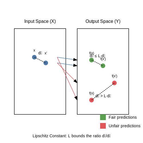
Individual fairness requires that similar individuals receive similar predictions from a machine learning model, formalized by Dwork et al. (2012) as a Lipschitz condition on the model's output space. Given a metric space (X, d) and a model f: X → Y, individual fairness holds if:
where L is the Lipschitz constant, d_X measures similarity in input space, and d_Y measures disparity in outcomes. Violations occur when two individuals with d_X(x, x') ≈ 0 receive significantly different predictions (d_Y ≫ 0).
Consistency Metric
The consistency score (Zemel et al., 2013) quantifies individual fairness by examining the k-nearest neighbors of each instance:
where N_k(x_i) denotes the k-nearest neighbors of x_i in feature space. Lower values indicate better fairness, with 0 representing perfect consistency. This metric is sensitive to the choice of distance metric for d_X – typically Euclidean or Mahalanobis distance for continuous features, or Hamming distance for categorical data.
Counterfactual Fairness
Kusner et al. (2017) propose testing individual fairness through counterfactuals: a model satisfies counterfactual fairness if:
for all individuals x and all protected attribute values a, a'. Here, y_{A←a} denotes the counterfactual outcome had the protected attribute been a. Practical implementation requires causal modeling to estimate these counterfactual distributions.
Fairness Through Awareness
This framework operationalizes individual fairness via two key components:
- Task-specific metric learning: Construct d_X through domain knowledge or metric learning techniques to capture legally/socially relevant similarities
- Fairness constraints: Enforce the Lipschitz condition during model training through regularization terms like:
where λ controls the fairness-accuracy trade-off. The pairwise computation scales quadratically with dataset size, requiring approximation techniques for large-scale applications.
Implementation Challenges
Key practical considerations when applying individual fairness metrics:
- Metric design: The choice of d_X is critical but non-trivial – poor metrics may encode existing biases
- Computational complexity: Pairwise comparisons become prohibitive for large datasets (O(n²) scaling)
- Causal vs. correlative: Most implementations rely on observable features rather than underlying causal structures
- Group-individual tradeoffs: Optimizing for individual fairness may worsen group fairness metrics like demographic parity
Recent work addresses these challenges through techniques like metric learning (Yurochkin et al., 2020), federated fairness constraints (Hu et al., 2021), and causal individual fairness (Pfohl et al., 2022).
3. Data Preprocessing for Fairness
Data Preprocessing for Fairness
Fairness in machine learning begins with the data pipeline. Biases embedded in training data propagate through models, necessitating rigorous preprocessing techniques to mitigate discriminatory patterns before model training. Advanced practitioners must address representation imbalances, proxy discrimination, and measurement biases through statistical and algorithmic interventions.
Identifying Protected Attributes
Sensitive attributes like race, gender, or age require careful handling. Direct removal often proves insufficient due to:
- Proxy variables: Features correlating with protected attributes (e.g., ZIP codes correlating with race)
- Intersectional bias: Compound discrimination across multiple attributes
- Measurement bias: Systemic errors in data collection processes
where \( \rho_{X,S} \) quantifies correlation between feature \( X \) and sensitive attribute \( S \). Features with \( |\rho_{X,S}| > \tau \) (typically τ=0.1) warrant mitigation.
Reweighting Techniques
Instance reweighting adjusts sample importance to balance outcomes across groups. For binary protected attribute \( S \) and target \( Y \):
This creates a pseudo-dataset where \( S \perp Y \). For continuous targets, kernel density estimation extends the approach:
Disparate Impact Removal
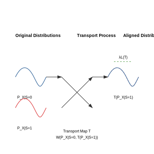
Optimal transport methods transform feature distributions to match across groups while preserving utility. The Wasserstein-based optimization:
where \( T \) is a transport map and \( \mathcal{L} \) preserves prediction-relevant information. Implementations use Sinkhorn iterations for computational efficiency.
Counterfactual Augmentation
Generative adversarial networks synthesize counterfactual examples by perturbing protected attributes while holding other features constant. The objective:
where \( G \) generates samples with modified \( s' \). This expands coverage of the data manifold for underrepresented groups.
Fairness-Aware Feature Selection
Multi-objective optimization selects features that maximize predictive power while minimizing dependence on protected attributes:
where \( X_\theta \) denotes the selected feature subset. Greedy algorithms or genetic optimization solve this NP-hard problem efficiently.
Practical implementations require careful monitoring of tradeoffs between fairness metrics (demographic parity, equalized odds) and model performance. Preprocessing alone cannot guarantee fairness but establishes necessary conditions for subsequent in-processing techniques.
3.2 Model Training and Fairness Constraints
Integrating fairness constraints into model training requires modifying the optimization objective to account for disparities across protected groups. Traditional machine learning minimizes a loss function L(θ) over parameters θ, but fairness-aware training introduces additional constraints or regularization terms.
Constrained Optimization Framework
The fairness-constrained optimization problem can be formulated as:
where Mk(θ) represents fairness metrics (e.g., demographic parity difference, equalized odds) for protected attribute k, and εk is the tolerance threshold. For differentiable constraints, this can be solved using Lagrangian multipliers or projected gradient descent.
Regularization Approaches
An alternative approach incorporates fairness as a regularization term:
where Rk(θ) penalizes unfairness (e.g., covariance between predictions and sensitive attributes) and λ controls the fairness-accuracy tradeoff. Common implementations include:
- Prejudice remover: Adds a discrimination-aware regularization term to logistic regression
- Adversarial debiasing: Uses a minimax game between predictor and adversary networks
- Fairness-aware gradient boosting: Modifies splitting criteria to reduce disparate impact
In-Processing Techniques
Several specialized algorithms enforce fairness during training:
Reductions Approach
Reductions transform fairness constraints into weighted classification problems. For example, the exponentiated gradient reduction:
adapts instance weights wi to satisfy constraints, where η is the learning rate.
Fair Robust Optimization
This method optimizes for worst-case performance across subgroups:
where G represents protected groups and Lg is the group-specific loss.
Implementation Considerations
Practical challenges in fairness-constrained training include:
- Non-convexity: Many fairness metrics lead to non-convex optimization landscapes
- Constraint conflicts: Some fairness definitions are mutually incompatible
- Computational overhead: Constraint satisfaction may require multiple passes over data
Recent advances address these through surrogate constraints, stochastic optimization, and parallelized computation. The choice of method depends on model architecture, fairness definition, and computational budget.

3.3 Post-processing Techniques
Post-processing techniques modify a model's predictions after training to improve fairness without altering the underlying model. These methods are particularly useful when retraining the model is impractical or when deploying pre-trained models in fairness-critical applications.
Probability Threshold Adjustment
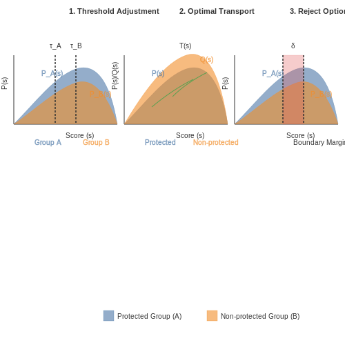
Given a binary classifier producing scores s ∈ [0,1], threshold adjustment enforces demographic parity or equalized odds by selecting group-specific thresholds τg. For a sensitive attribute A with groups g ∈ G, the adjusted predictions ŷ become:
The thresholds τg are optimized to satisfy fairness constraints while minimizing utility loss. For equalized odds, thresholds are chosen such that:
Optimal Transport for Fairness
Optimal transport theory provides a principled way to redistribute probability mass across groups. Let Pg(s) be the score distribution for group g. We solve for a transport map T that transforms Pg to match a target distribution Q while minimizing the Wasserstein distance:
where c is a cost function (typically L2 distance) and T# denotes the pushforward measure. The target Q can enforce statistical parity by setting Q = P (the overall population distribution).
Reject Option Classification
This technique identifies uncertain predictions near the decision boundary and assigns them favorable outcomes for disadvantaged groups. For a margin δ, predictions are modified as:
The margin δ controls the trade-off between fairness and accuracy. Empirical studies show this method particularly effective when the base classifier exhibits bias in boundary region predictions.
Calibration Preservation
While many post-processing methods improve fairness at the cost of calibration, simultaneous calibration-preserving techniques exist. For a score s and group g, we learn an isotonic regression model fg such that:
The calibrated scores fg(s) maintain both fairness and the probabilistic interpretation of model outputs. This is crucial in applications like healthcare where well-calibrated risk scores are required.
Implementation Considerations
Key challenges in deploying post-processing methods include:
- Group overlap: Techniques assume non-overlapping groups, requiring careful handling of intersectional identities
- Data drift: Thresholds and transformations may need periodic recalibration as input distributions shift
- Multi-objective tradeoffs: Pareto optimization frameworks can balance fairness, accuracy, and other metrics
Recent advances include differentiable post-processing layers that can be fine-tuned end-to-end while maintaining fairness guarantees. These approaches combine the flexibility of post-processing with some benefits of in-processing methods.
4. Fairness in Credit Scoring
Fairness in Credit Scoring
Credit scoring models are widely deployed in financial institutions to assess the creditworthiness of applicants. However, these models can inadvertently introduce or amplify biases, leading to disparate outcomes across demographic groups. Evaluating fairness in credit scoring requires rigorous statistical metrics that quantify disparities in model performance across protected attributes such as race, gender, or age.
Disparate Impact and Statistical Parity
Disparate impact measures whether a model’s predictions disproportionately favor one group over another. It is quantified as the ratio of approval rates between protected and unprotected groups:
where Ŷ is the model’s prediction (e.g., loan approval), and A is the protected attribute. A value of 1 indicates perfect fairness, while values below 0.8 (the "80% rule") may indicate discrimination under U.S. employment law guidelines.
Equalized Odds and Predictive Parity
Equalized odds requires that true positive rates (TPR) and false positive rates (FPR) be equal across groups:
Predictive parity, on the other hand, ensures that the positive predictive value (PPV) is equal across groups:
Violations of these conditions indicate that the model’s errors are unevenly distributed, potentially disadvantaging certain groups.
Individual Fairness Metrics
Individual fairness ensures that similar individuals receive similar predictions, regardless of group membership. A common measure is the Lipschitz condition:
where f is the scoring model, d is a distance metric, and L is a constant. Enforcing this condition mitigates arbitrary disparities between similar applicants.
Case Study: Bias Mitigation in FICO Scoring
In a 2019 study, FICO scores were found to exhibit racial disparities due to historical biases in training data. Mitigation strategies included:
- Reweighting training samples to balance representation.
- Adversarial debiasing to minimize correlation between predictions and protected attributes.
- Post-processing adjustments to equalize approval thresholds across groups.
These interventions reduced disparate impact from 0.72 to 0.89 while maintaining predictive accuracy.
Trade-offs Between Fairness and Accuracy
Optimizing for fairness often reduces model accuracy due to the impossibility theorem in fairness-aware learning, which states that no model can simultaneously satisfy all fairness criteria (e.g., independence, separation, sufficiency) unless the data is perfectly unbiased. Practitioners must carefully select fairness constraints based on regulatory requirements and ethical priorities.
Fairness in Hiring Algorithms
Hiring algorithms are increasingly deployed to automate resume screening, candidate ranking, and interview selection. However, these systems can inadvertently perpetuate or amplify biases present in historical hiring data. Evaluating fairness in hiring algorithms requires specialized metrics that account for both statistical parity and disparate impact across protected groups (e.g., gender, race, age).
Key Fairness Metrics for Hiring
The following metrics are critical for assessing fairness in hiring algorithms:
- Demographic Parity: Measures whether selection rates are equal across groups. Defined as:
where Ŷ is the predicted hire (1) or reject (0), and A represents the protected attribute.
- Equalized Odds: Requires equal true positive rates (TPR) and false positive rates (FPR) across groups:
- Predictive Parity: Ensures equal precision across groups, i.e., the probability of being a qualified hire given a positive prediction:
Disparate Impact Analysis
The four-fifths rule, derived from U.S. employment law, quantifies disparate impact as:
A ratio below 0.8 suggests potential discrimination. For example, if male applicants are hired at 20% and female applicants at 12%, the ratio is 0.6, indicating bias.
Real-World Case Study: Amazon's Recruiting Engine
Amazon's AI recruiting tool (2014-2017) learned to penalize resumes containing words like "women's" or graduates from all-women colleges. The system was trained on historical hiring data dominated by male candidates, causing it to replicate this bias. Post-hoc analysis revealed:
- Demographic parity violation: Female candidates had 30% lower selection probability
- Disparate impact ratio of 0.65 for technical roles
Mitigation Strategies
Effective approaches for fair hiring algorithms include:
- Pre-processing: Reweighting training data to balance group representation
- In-processing: Adding fairness constraints to the loss function during model training
- Post-processing: Adjusting decision thresholds per group to achieve equalized odds
where λ controls the fairness-accuracy tradeoff.
Audit Frameworks
Practical auditing requires:
- Slice-aware evaluation across intersectional groups (e.g., Black women vs. white men)
- Counterfactual testing (how predictions change when protected attributes are modified)
- Continuous monitoring for concept drift in fairness metrics
4.3 Fairness in Healthcare Predictive Models
Healthcare predictive models must address fairness to avoid exacerbating disparities in diagnosis, treatment allocation, and resource distribution. Unlike generic fairness metrics, healthcare applications require domain-specific considerations due to the high-stakes nature of medical decisions and the sensitive interplay between demographic variables and biological factors.
Challenges in Healthcare Fairness
Healthcare datasets often exhibit:
- Imbalanced representation of racial, ethnic, and socioeconomic groups in training data
- Proxy discrimination where variables like ZIP code correlate with protected attributes
- Differential measurement error where diagnostic tools have varying accuracy across populations
For example, pulse oximeters overestimate oxygen saturation in patients with darker skin tones, creating biased training data for respiratory failure prediction models.
Clinical Fairness Metrics
Standard fairness metrics require adaptation for clinical contexts:
where Y represents the true clinical outcome and A the protected attribute. In healthcare, we often need outcome-conditional rather than decision-conditional fairness due to the ethical imperative to prioritize patient outcomes over algorithmic decisions.
Case Study: Kidney Allocation
The US kidney transplant system uses a predictive model (KDPI) that originally disadvantaged Black patients due to:
- Race-adjusted creatinine thresholds in kidney function estimation
- Geographic disparities in organ availability
- Socioeconomic barriers to pre-transplant care
The revised 2021 model removed race coefficients and incorporated:
This change reduced the waitlist disparity ratio from 1.43 to 1.12 between Black and white patients.
Multi-Objective Optimization
Healthcare models must balance competing objectives:
where ΔEO measures equalized odds violation and ΔDP demographic parity violation. The Pareto frontier represents optimal trade-offs between accuracy and fairness constraints.
Longitudinal Fairness
Healthcare requires temporal fairness evaluation due to:
- Delayed effects of treatment recommendations
- Changing patient conditions over time
- Feedback loops in clinical decision support systems
The longitudinal fairness metric evaluates disparities in cumulative outcomes:
where Yt represents the outcome at time t and T the evaluation horizon.
5. Trade-offs Between Fairness and Accuracy
5.1 Trade-offs Between Fairness and Accuracy
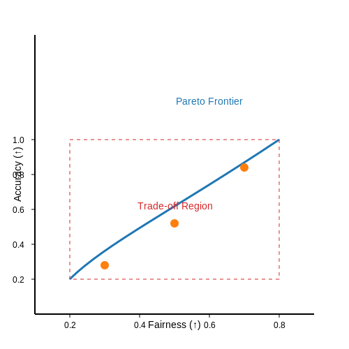
The relationship between fairness and accuracy in machine learning models is inherently adversarial. Optimizing for one often comes at the expense of the other, creating a Pareto frontier where improvements in fairness reduce accuracy and vice versa. This trade-off arises because fairness constraints typically restrict the model's hypothesis space, preventing it from exploiting statistical patterns that may correlate with protected attributes.
Mathematical Formulation
Consider a binary classification task where Y ∈ {0,1} is the true label and Ŷ ∈ {0,1} is the predicted label. Let A ∈ {0,1} represent a binary protected attribute (e.g., gender or race). The accuracy-fairness trade-off can be formalized as an optimization problem:
where f is the classifier, ℱ is the hypothesis space, and ϵ controls the strictness of the demographic parity constraint. As ϵ → 0, the fairness constraint becomes stricter, typically increasing the minimum achievable error rate.
Empirical Evidence
Multiple studies have quantified this trade-off across different domains:
- In credit scoring, enforcing equal opportunity fairness reduced accuracy by 3-8% on major lending datasets.
- For COMPAS recidivism predictions, achieving statistical parity decreased AUC from 0.71 to 0.68.
- In facial recognition, gender classification accuracy dropped 15% when requiring equal false positive rates across genders.
Theoretical Bounds
Under certain conditions, the fairness-accuracy trade-off can be characterized theoretically. For a binary classifier with base rate p = P(Y=1), the maximum possible accuracy while satisfying perfect demographic parity is:
where p0 and p1 are the base rates for each protected group. This shows that the accuracy penalty grows with the disparity in base rates between groups.
Mitigation Strategies
Several approaches attempt to navigate this trade-off:
- Pareto optimization: Identifying the set of non-dominated solutions where neither fairness nor accuracy can be improved without degrading the other.
- Adaptive reweighting: Dynamically adjusting instance weights during training to balance fairness and accuracy objectives.
- Fair representation learning: Learning embeddings that decorrelate protected attributes from other features while preserving predictive information.
The choice of strategy depends on the application context and the relative importance of fairness versus accuracy in the deployment environment. In high-stakes domains like criminal justice or healthcare, even significant accuracy reductions may be justified to ensure equitable treatment across demographic groups.
5.2 Scalability of Fairness Metrics
As machine learning models are increasingly deployed in large-scale, real-world applications, the computational efficiency of fairness metrics becomes critical. Many fairness metrics, while theoretically sound, suffer from poor scalability due to high computational complexity or memory requirements when applied to massive datasets or high-dimensional feature spaces.
Computational Complexity Analysis
Consider the demographic parity difference (DPD) metric, which compares selection rates between protected groups. For binary classification with k protected groups and n instances, the computational complexity is:
While linear in the number of instances, this becomes problematic when n grows into the millions or billions. More complex metrics like equalized odds require computing confusion matrices for each protected group:
where c represents the number of classes. For multi-class problems with many protected groups, this complexity grows rapidly.
Approximation Techniques for Large-Scale Applications
Several approaches have been developed to maintain fairness guarantees while improving scalability:
- Stratified sampling: Compute metrics on carefully constructed representative subsets rather than the full population
- Online computation: Update fairness metrics incrementally as new data arrives, avoiding full recomputation
- Distributed computation: Parallelize fairness calculations across multiple nodes using frameworks like Spark or Dask
Online Fairness Monitoring
The online version of demographic parity can be computed using exponential moving averages:
where α is a smoothing factor and yt is the prediction at time t. This reduces the space complexity from O(n) to O(1) while providing reasonable approximations.
Dimensionality Challenges
High-dimensional feature spaces introduce additional scalability concerns. Intersectional fairness metrics that consider combinations of protected attributes face exponential growth in computational requirements:
where m is the number of protected attributes, each with ki possible values. Techniques like:
- Attribute clustering
- Dimensionality reduction
- Fairness-aware feature selection
can help mitigate these challenges while preserving meaningful fairness assessments.
Practical Implementation Considerations
When implementing fairness metrics at scale, several practical factors must be considered:
- Memory efficiency: Avoid storing multiple copies of large datasets for different protected groups
- Numerical stability: Ensure stable calculations when dealing with very small subgroup populations
- Parallelization overhead: Balance the cost of distributed computation against the benefits
Modern ML frameworks are beginning to incorporate optimized fairness metric implementations. For example, TensorFlow's Fairness Indicators uses:
- Binning techniques for efficient histogram calculations
- Asynchronous computation pipelines
- Memory-mapped storage for large result sets
5.3 Cultural and Contextual Variations
Fairness metrics in machine learning must account for cultural and contextual differences to avoid imposing a one-size-fits-all standard. What constitutes fairness in one demographic or geographic setting may not hold in another due to varying social norms, legal frameworks, and historical inequities. For instance, a model trained to allocate loans in the U.S. may require different fairness adjustments than one deployed in India, where caste-based disparities necessitate distinct considerations.
Cultural Bias in Dataset Composition
Datasets often reflect the biases of their creators, leading to underrepresentation or misrepresentation of certain groups. For example, facial recognition systems trained primarily on lighter-skinned individuals exhibit higher error rates for darker-skinned faces. This disparity arises from imbalanced training data rather than inherent algorithmic limitations. The disparate impact can be quantified using statistical parity difference (SPD):
where A denotes the sensitive attribute (e.g., race or gender), and Ŷ is the model's prediction. A non-zero SPD indicates bias, but the acceptable threshold varies by context. In hiring algorithms, a 4/5ths rule (80% selection rate parity) is commonly used in the U.S., while other regions may enforce stricter or looser standards.
Contextual Adaptations of Fairness Metrics
Equalized odds and demographic parity may conflict in practice. Consider a healthcare model predicting disease risk: enforcing strict demographic parity could lead to overdiagnosis in low-risk populations or underdiagnosis in high-risk ones. Instead, equalized odds ensures similar true positive rates across groups:
However, in cultures where certain diseases are stigmatized, even equalized odds may be insufficient. For example, mental health predictions in conservative societies might require additional privacy safeguards to prevent discriminatory outcomes.
Case Study: Credit Scoring in Global Markets
In Nigeria, traditional credit scoring models fail to account for informal economies, where many transactions occur outside banking systems. Alternative fairness metrics incorporate community-based trust networks, a practice irrelevant in countries with formalized credit histories. Here, counterfactual fairness provides a framework to adjust for contextual variables:
This ensures predictions remain invariant to sensitive attributes under hypothetical interventions, adapting to local economic structures.
Legal and Normative Constraints
The EU’s GDPR mandates "right to explanation" for automated decisions, requiring interpretability metrics alongside fairness. In contrast, China’s AI governance emphasizes collective welfare over individual parity, influencing how fairness is quantified. Models must dynamically adjust to such constraints—e.g., using contextual bandits to balance fairness and utility under region-specific regulations.
6. Key Research Papers
6.1 Key Research Papers
- Fairness issues, current approaches, and challenges in ... - Springer — The rest of the research question answers are regarding the analysis of the filtered papers. The research problems discussed in ... 6.3.4 Incorporating accuracy and fairness metrics. Usually, any ML models follow accuracy matrices for developing the model. ... It is widely used in healthcare research. the key characteristics of this dataset are ...
- Fairness in Machine Learning: A Survey | ACM Computing Surveys — Now, we focus on more general challenges for the domain as a set of five dilemmas for future research (the ordering is coincidental): Dilemma-1: Balancing the tradeoff between fairness and model performance (Section 6.1); Dilemma-2: Quantitative notions of fairness permit model optimization, yet cannot balance different notions of fairness ...
- Fairness metrics and bias mitigation strategies for rating predictions — Based on an analysis of fairness metrics used in machine learning and a discussion of their applicability in the recommender system domain, we map the proposed metrics from the two domains and identify commonly used concepts and definitions of fairness. ... Bias that happens during model evaluation. Buolamwini (2017) and Suresh and Guttag (2019 ...
- Quantifying Social Biases in NLP: A Generalization and Empirical ... — Abstract. Measuring bias is key for better understanding and addressing unfairness in NLP/ML models. This is often done via fairness metrics, which quantify the differences in a model's behaviour across a range of demographic groups. In this work, we shed more light on the differences and similarities between the fairness metrics used in NLP. First, we unify a broad range of existing metrics ...
- PDF Evaluating the Quality of Machine Learning Explanations: A Survey on ... — This review focuses on metrics for evaluating ML ex-planations, including both human-centred subjective evaluations and quantitative objec-tive evaluations that are not fully investigated in the current review papers. To the best of our knowledge, this is the first survey that specifically reports on the quality evaluation of ML explanations.
- (PDF) Evaluation Metrics and Evaluation - ResearchGate — Usage of evaluation metrics includes things like accuracy, precision, recall, area under the curve (AUC), and F1-score. According to the findings, improving hyper-parameters results in an 18% ...
- PDF Fairness Issues, Current Approaches, and Challenges in Machine ... - Rivas — potential future direction in ML and AI fairness. Keywords: ethics, model fairness, bias reduction, fair prediction, AI, machine-learning 1 Introduction Machine learning-based models have undoubtedly brought remarkable advancements in various fields, demonstrating their ability to make accurate predictions and auto-mate decision-making processes.
- (PDF) Evaluating the Quality of Machine Learning ... - ResearchGate — The paper concludes that the evaluation of ML explanations is a multidisciplinary research topic. It is also not possible to define an implementation of evaluation metrics, which can be applied to ...
- Common fairness metrics — Fairlearn 0.13.0.dev0 documentation — Fairness metrics like demographic parity can also be used as optimization constraints during the machine learning model training process. However, demographic parity may not be well-suited for this purpose because it does not place requirements on the exact distribution of predictions with respect to other important variables.
6.2 Books and Comprehensive Guides
- Assessing fairness in machine learning models: A study of racial bias ... — Similar results were observed with the MLP model (F1: 0.513 vs. 0.535 vs. 0.526, and sensitivity: 0.503 vs. 0.488 vs. 0.480) in the performance comparisons, and there were no significant differences in fairness evaluation approaches, with p-values of 0.466 in Δ f 1 and 0.596 in Δ Se, respectively.
- PDF Machine Learning Evaluation — Part II Evaluation for Classification 5 Metrics 83 5.1 Overview of the Problem 83 5.2 An Ontology of Performance Measures 86 5.3 Illustrative Example 88 5.4 Performance Metrics with a Multi-class Focus 90 5.5 Performance Metrics with a Single-Class Focus 98 5.6 Skew/Imbalances, Cost, Uncertainty, and Calibration 110 5.7 More Details on ROC ...
- Fairness metrics and bias mitigation strategies for rating predictions — In general, while the target fairness metric can be improved by the bias mitigation approach in most cases, other fairness metrics might be decreased or increased at the same time. Third, the impact of fairness improvements on predictive performance in the rating prediction scenario, measured by RMSE and MAE, also depends on the specific bias ...
- Performance Evaluation Metrics - SpringerLink — 5.1.2 Taxonomy of Classifier Evaluation Metrics. Depending on the model that you are developing there will be a set of common evaluation metrics used to evaluate its performance as shown in Fig. 5.1. These are typically split into supervised and un-supervised categories.
- (PDF) Counterpart Fairness -- Addressing Systematic between-group ... — the fairness of algorithmic decisions and help train fairer ML models. The choice of fairness evaluation metrics will depend on the specific usage and the desired lev el of fairness.
- Fairness in Machine Learning — Fairlearn 0.13.0.dev0 documentation — For example, group fairness metrics do not account for differences in individual experiences, nor do they account for procedural justice. In some scenarios, fairness metrics such as demographic parity and equalized odds cannot be satisfied at the same time. At a first glance, this may appear to be a mathematical problem.
- Fairness in Machine Learning: A Survey | ACM Computing Surveys — Other works considering fairness from either the consumer or provider side include the analysis of different recommendation strategies for a variety of (fairness) metrics , subset-based evaluation metrics to measure the utility of recommendations for different groups (e.g., based on demographics) , and a general framework to optimize utility ...
- Common fairness metrics — Fairlearn 0.13.0.dev0 documentation — The goal of the equalized odds fairness metric is to ensure a machine learning model performs equally well for different groups. It is stricter than demographic parity because it requires that the machine learning model's predictions are not only independent of sensitive group membership, but that groups have the same false positive rates and ...
- Applied Causal Inference - 8 Model Fairness - GitHub Pages — Specifically, this section covers causal techniques that aid in the assessment of model fairness as well as the creation of fair models. We will discuss the need for causal methods instead of standard statistical tools when evaluating potentially discriminatory effects. 8.1 Introduction to Model Fairness 8.1.1 Prerequisite Knowledge
- Fairness issues, current approaches, and challenges in ... - Springer — With the increasing influence of machine learning algorithms in decision-making processes, concerns about fairness have gained significant attention. This area now offers significant literature that is complex and hard to penetrate for newcomers to the domain. Thus, a mapping study of articles exploring fairness issues is a valuable tool to provide a general introduction to this field. Our ...
6.3 Online Resources and Tools
- Fairness Score and process standardization: framework for fairness ... — While we create a certification framework and identify fairness metrics, it is necessary to define fairness. AI fairness is a rapidly growing topic of inquiry [].References [25,26,27] proposed multiple definitions of fairness.Reference [] proposed some definitions for formalizing fairness from other disciplines.In some cases, defining fairness comes as a legal compulsion, for example, lending ...
- Fairness metrics and bias mitigation strategies for rating predictions — Based on an analysis of fairness metrics used in machine learning and a discussion of their applicability in the recommender system domain, we map the proposed metrics from the two domains and identify commonly used concepts and definitions of fairness. ... Bias that happens during model evaluation. Buolamwini (2017) and Suresh and Guttag (2019 ...
- How can we manage biases in artificial intelligence systems - A ... — IBM's AI Fairness 360 toolkit is a holistic and comprehensive approach that includes 70 parameter fairness metrics to reduce biases in AI systems (Bellamy et al., 2019). In healthcare systems to decrease the bias by creating fairness standards, regulating algorithms, tools for clinical decision making and fostering relationship between public ...
- Chapter 11 Bias and Fairness | Big Data and Social Science — 11.1 Introduction. In Chapter Machine Learning, you learned about several of the concepts, tools, and approaches used in the field of machine learning and how they can be applied in the social sciences.In that chapter, we focused on evaluation metrics such as precision (positive predictive value), recall (sensitivity), area-under-curve (AUC), and accuracy, that are often used to measure the ...
- Fairness in Machine Learning: A Survey | ACM Computing Surveys — Other works considering fairness from either the consumer or provider side include the analysis of different recommendation strategies for a variety of (fairness) metrics , subset-based evaluation metrics to measure the utility of recommendations for different groups (e.g., based on demographics) , and a general framework to optimize utility ...
- Evaluation Metrics in Machine Learning - GeeksforGeeks — Greater the value of AUCC better the performance of the model. ROC Curve for Evaluation of Classification Models Precision. There is another metric named Precision. Precision is a measure of a model's performance that tells you how many of the positive predictions made by the model are actually correct. \rm{Precision} = \frac{TP}{TP\; +\; FP ...
- Survey on Machine Learning Biases and Mitigation Techniques - MDPI — Machine learning (ML) has become increasingly prevalent in various domains. However, ML algorithms sometimes give unfair outcomes and discrimination against certain groups. Thereby, bias occurs when our results produce a decision that is systematically incorrect. At various phases of the ML pipeline, such as data collection, pre-processing, model selection, and evaluation, these biases appear ...
- Fairness issues, current approaches, and challenges in ... - Springer — With the increasing influence of machine learning algorithms in decision-making processes, concerns about fairness have gained significant attention. This area now offers significant literature that is complex and hard to penetrate for newcomers to the domain. Thus, a mapping study of articles exploring fairness issues is a valuable tool to provide a general introduction to this field. Our ...
- Modular Federated Learning: A Meta-Framework Perspective - arXiv.org — Proposes a novel taxonomy for interpretable federated learning, covering methods that enhance prediction explainability, enable model debugging, and attribute contributions to data owners, crucial for fair reward allocation. Includes a comprehensive analysis of current approaches, evaluation metrics, and future research directions.
- The statistical fairness field guide: perspectives from social and ... — Over the past several years, a multitude of methods to measure the fairness of a machine learning model have been proposed. However, despite the growing number of publications and implementations, there is still a critical lack of literature that explains the interplay of fair machine learning with the social sciences of philosophy, sociology, and law. We hope to remedy this issue by ...