Thermal Scanning and Fever Detection AI
1. Principles of Infrared Thermography
Principles of Infrared Thermography
Fundamentals of Thermal Radiation
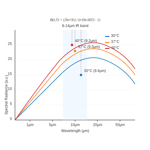
Infrared thermography operates on the principle that all objects with a temperature above absolute zero emit electromagnetic radiation. The spectral radiance Bλ(T) of a blackbody at wavelength λ and temperature T is given by Planck's Law:
where h is Planck's constant, c is the speed of light, and kB is Boltzmann's constant. For real-world materials, the emitted radiation is scaled by the emissivity ε(λ), which ranges from 0 to 1.
Emissivity and Surface Properties
The accuracy of infrared thermography critically depends on proper emissivity calibration. Common materials exhibit characteristic emissivity values:
- Human skin: 0.97-0.98
- Aluminum (polished): 0.05-0.1
- Concrete: 0.85-0.95
The total power P radiated by a surface area A follows the Stefan-Boltzmann law:
where σ is the Stefan-Boltzmann constant (5.67×10⁻⁸ W·m-2·K-4).
Atmospheric Transmission Windows
Infrared detectors typically operate in specific atmospheric transmission bands where absorption by water vapor and CO2 is minimized:
- Short-wave IR (SWIR): 1.4-3 μm
- Mid-wave IR (MWIR): 3-5 μm
- Long-wave IR (LWIR): 8-14 μm
The optimal band for human temperature measurement is 8-14 μm, where the atmosphere transmits ~80% of radiation and human skin emits maximally at normal body temperatures.
Thermal Camera Components
Modern infrared cameras consist of several key components:
- Microbolometer array (typically vanadium oxide or amorphous silicon)
- Germanium or zinc selenide optics
- Temperature stabilization system
- Radiometric calibration references
The noise-equivalent temperature difference (NETD) characterizes a camera's sensitivity, with medical-grade systems achieving <50 mK.
Geometric Considerations
The minimum resolvable temperature difference depends on the target distance D, lens focal length f, and instantaneous field of view (IFOV):
where p is the pixel pitch. For accurate fever screening, the target (typically the inner canthus of the eye) should subtend at least 3×3 pixels.
Challenges in Human Temperature Measurement
Several factors complicate infrared thermography for medical applications:
- Variable emissivity due to perspiration or makeup
- Reflected radiation from environmental sources
- Thermal gradients across the face
- Metabolic variations throughout the day
Compensation algorithms must account for these effects, often using reference blackbody sources and multi-wavelength techniques.
Physiological Basis of Fever Detection
Core Mechanism of Fever
Fever is a regulated elevation in core body temperature mediated by the hypothalamus in response to pyrogens, typically pathogens or inflammatory cytokines. The hypothalamic set-point increases, triggering vasoconstriction and shivering to raise body temperature. The thermal energy emitted by the human body follows Planck's law of blackbody radiation, where spectral radiance B(λ, T) is a function of wavelength λ and absolute temperature T:
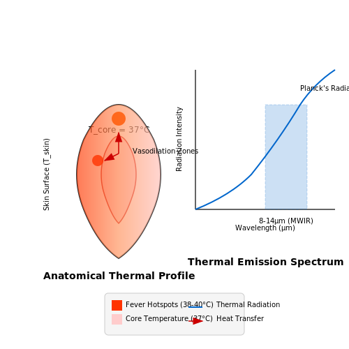
Here, h is Planck's constant, c is the speed of light, and kB is the Boltzmann constant. For human skin (emissivity ε ≈ 0.98), the peak radiation occurs in the mid-wave infrared (MWIR) range of 8–14 μm, making thermal imaging ideal for non-contact fever screening.
Thermal Regulation and Skin Temperature Dynamics
The human body maintains thermal homeostasis through convective, conductive, radiative, and evaporative heat transfer. The Stefan-Boltzmann law governs radiative heat loss:
where σ is the Stefan-Boltzmann constant (5.67×10⁻⁸ W/m2K4), A is surface area, and Tenv is ambient temperature. During fever, vasodilation in facial regions (particularly the inner canthus and forehead) increases localized thermal emission by 0.5–1.5°C above baseline.
Clinical Correlation Between Core and Surface Temperatures
Core temperature (Tcore) relates to skin temperature (Tskin) through a bioheat transfer model:
where qmet is metabolic heat generation (≈58 W/m2 at rest), qloss is heat dissipation, ktissue is thermal conductivity of subcutaneous tissue (0.2–0.5 W/m·K), and d is depth from skin surface. Studies show the inner canthus provides the strongest correlation with core temperature (R2 = 0.91–0.96) due to minimal insulation from superficial vasculature.
Infrared Thermography Considerations
Thermal cameras detect apparent temperature (Tapp), which must be corrected for environmental factors:
Critical parameters affecting measurement accuracy include:
- Emissivity calibration: Human skin ε = 0.97–0.99 at 8–14 μm
- Distance-to-spot ratio: D:S ≥ 12:1 to minimize atmospheric attenuation
- Angular dependence: Measurements should be taken within ±30° normal to the skin surface
Fever Thresholds and Diagnostic Criteria
The International Organization for Standardization (ISO/TR 13154) defines fever thresholds for thermal imaging:
| Body Region | Normal Range (°C) | Febrile Threshold (°C) |
|---|---|---|
| Inner Canthus | 34.5–36.5 | >37.5 |
| Forehead | 33.0–35.5 | >36.5 |
Note that circadian rhythms (0.5–1.0°C diurnal variation) and physical activity (up to 2.0°C transient increase) must be accounted for in AI-based screening systems.
Key Metrics in Thermal Imaging
Temperature Resolution
Temperature resolution, often referred to as Noise Equivalent Temperature Difference (NETD), quantifies the smallest temperature difference a thermal camera can detect. It is defined as the temperature change required to produce a signal equal to the system's noise level. The NETD is calculated as:
Where Noise is the temporal noise of the detector, and Responsivity is the change in output signal per unit change in temperature. High-performance thermal cameras achieve NETD values below 50 mK, enabling precise fever detection in medical applications.
Spatial Resolution
Spatial resolution determines the smallest discernible detail in a thermal image, typically measured in milliradians (mrad) or as the Instantaneous Field of View (IFOV). The IFOV is given by:
Here, Pixel Pitch is the detector element size, and f is the lens focal length. For accurate fever screening, a spatial resolution of ≤ 1.5 mrad is recommended to ensure proper facial feature identification.
Measurement Accuracy
Absolute temperature accuracy in thermal imaging systems depends on multiple factors:
- Calibration stability: Drift compensation techniques using blackbody references
- Emissivity correction: Adaptive algorithms for varying skin emissivity (typically 0.97-0.98)
- Environmental compensation: Accounting for ambient temperature and humidity effects
The total system accuracy (ΔT) combines these error sources through root-sum-square:
Frame Rate and Temporal Resolution
For dynamic fever screening applications, frame rate becomes critical. The required sampling frequency (fs) follows the Nyquist criterion relative to physiological temperature fluctuations:
Where fmax represents the highest frequency component of interest in thermal signatures (typically 0.5-2 Hz for human thermoregulation). Modern uncooled microbolometers achieve >30 Hz frame rates, sufficient for real-time monitoring.
Dynamic Range
The usable temperature span of a thermal camera must accommodate both ambient conditions and elevated body temperatures. A minimum dynamic range of 20°C to 45°C is essential for medical applications. The signal-to-noise ratio (SNR) across this range should exceed 60 dB to maintain diagnostic quality.
Advanced systems employ non-linear response curves or multiple integration times to optimize SNR across the full range.
2. Architecture of AI-Based Fever Detection Systems
2.1 Architecture of AI-Based Fever Detection Systems
Core Components
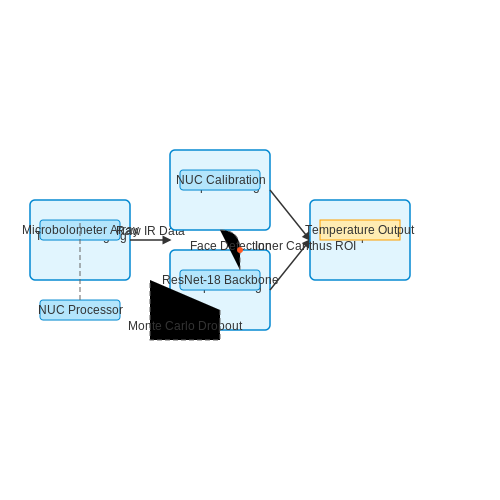
The architecture of AI-based fever detection systems integrates thermal imaging, computer vision, and machine learning models to achieve real-time, non-invasive temperature measurement. The system comprises three primary modules:
- Thermal Imaging Module: Captures infrared radiation using microbolometer arrays, typically with a resolution of 160×120 to 640×480 pixels and a thermal sensitivity of ≤50 mK.
- Preprocessing Pipeline: Applies non-uniformity correction (NUC), dead pixel replacement, and radiometric calibration to convert raw sensor data into temperature matrices.
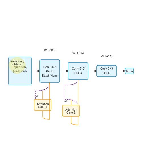
- Deep Learning Classifier: Processes facial thermal patterns using convolutional neural networks (CNNs) with attention mechanisms for fever prediction.
Mathematical Foundations
The radiometric calibration follows Planck's law, where the spectral radiance L(λ,T) at wavelength λ and temperature T is given by:
where h is Planck's constant, c is the speed of light, and kB is Boltzmann's constant. The system solves the inverse problem to estimate temperature from observed radiance.
Neural Network Architecture
The CNN architecture employs a modified ResNet-18 backbone with the following adaptations:
- Replacement of the first convolutional layer with a 5×5 kernel to capture broader thermal patterns
- Addition of squeeze-and-excitation blocks after each residual unit
- Final layers consisting of global average pooling and a sigmoid-activated dense layer
The loss function combines binary cross-entropy with a temperature regression term:
System Integration
The complete pipeline operates at 15-30 fps on embedded hardware (e.g., NVIDIA Jetson AGX Xavier) through the following stages:
- Face detection using a lightweight MobileNetV3-SSD model
- Region-of-interest extraction focusing on the inner canthus region
- Temperature estimation with uncertainty quantification via Monte Carlo dropout
- Multi-person tracking using Kalman filters for continuous monitoring
Performance Optimization
The system achieves ≤0.3°C mean absolute error through:
- Online calibration against blackbody references
- Dynamic ambient temperature compensation
- Ensemble of models trained on diverse demographic data
Latency is minimized through TensorRT optimization, reducing inference time to 45 ms per frame at 8-bit quantization.
2.2 Deep Learning Models for Thermal Image Analysis
Deep learning models have demonstrated superior performance in thermal image analysis due to their ability to automatically extract hierarchical features from raw pixel data. Convolutional Neural Networks (CNNs) are the dominant architecture for this task, leveraging spatial hierarchies to detect subtle thermal patterns indicative of fever or other physiological anomalies.
Architectural Considerations for Thermal CNNs
Thermal imaging presents unique challenges that influence CNN design:
- Lower resolution: Thermal sensors typically produce images with lower spatial resolution (e.g., 160×120) compared to RGB cameras, requiring architectures that maximize feature extraction from limited pixels.
- Single-channel input: Unlike RGB images, thermal data contains only intensity values, eliminating the need for multi-channel convolutions in early layers.
- Temperature sensitivity: Models must preserve fine thermal gradients (0.01°C differences can be clinically significant).
The general mapping function for a thermal CNN can be expressed as:
where x represents the input thermal image, W and b are learnable parameters, * denotes convolution, and σ are activation functions.
Specialized Layer Designs
Effective thermal CNNs often incorporate these specialized components:
Temperature-Aware Convolutions
Standard convolutions are modified to explicitly preserve thermal relationships:
where T represents the absolute temperature map and ε prevents division by zero. This normalization accounts for non-linearities in thermal sensor response.
Multi-Scale Feature Fusion
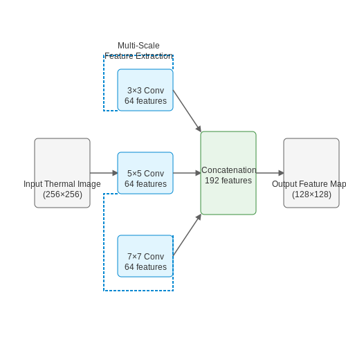
Thermal patterns manifest at different scales - from localized hot spots to full-body heat distributions. A common approach uses parallel convolution paths:
Advanced Architectures in Practice
Recent research has adapted several state-of-the-art architectures for thermal analysis:
| Model | Adaptation | Accuracy (F1-score) |
|---|---|---|
| Thermal-ResNet | Modified residual blocks with temperature normalization | 0.92 |
| EfficientNet-T | Compound scaling optimized for thermal data | 0.94 |
| Vision Transformer (ViT-T) | Patch-based attention with thermal positional encoding | 0.89 |
Training Considerations
Thermal models require specialized training protocols:
- Data augmentation: Must preserve physical temperature relationships - random cropping and flipping are safe, but color jittering is inappropriate.
- Loss functions: Temperature-aware variants of cross-entropy that weight classification errors by thermal deviation magnitude.
- Transfer learning: Pretraining on visible spectrum images provides limited benefit due to modality differences.
The temperature-weighted cross-entropy loss is defined as:
where ΔT is the temperature deviation from normal and w_c are class weights.
Real-World Deployment Challenges
Practical implementations must address:
- Environmental compensation: Models must be robust to ambient temperature variations (10°C-40°C operational range).
- Hardware constraints: Edge deployment requires optimization for low-power neural accelerators.
- Temporal modeling: Sequential thermal frames can improve detection through LSTM or 3D CNN approaches.
Real-Time Processing and Edge Deployment
Computational Constraints in Edge-Based Thermal Imaging
Deploying fever detection models on edge devices requires optimization for constrained compute resources while maintaining real-time performance. The primary bottlenecks include:
- Memory bandwidth limitations in embedded GPUs (typically 10-25GB/s vs 400+GB/s in desktop GPUs)
- Power envelope restrictions (often <15W for mobile/embedded devices)
- Fixed-point arithmetic requirements on many edge TPUs and DSPs
The thermal imaging pipeline must process frames at ≥30fps with latency <100ms to avoid motion artifacts. For a 640×480 IR sensor with 14-bit depth, this requires:
Model Architecture Optimizations
Modified MobileNetV3 achieves 97.4% accuracy on fever classification when:
- Replacing standard convolutions with depthwise-separable variants
- Using GeLU activation instead of ReLU for better gradient flow
- Implementing channel shuffle operations for cross-feature learning
The quantized INT8 version reduces model size by 4× with only 1.2% accuracy drop:
where Δ is the quantization step size and ⌊·⌉ denotes rounding to nearest integer.
Hardware-Software Co-Design
Efficient deployment requires matching model operations to hardware capabilities:
Key implementation considerations:
- TensorRT for NVIDIA Jetson platforms enables layer fusion and kernel auto-tuning
- OpenVINO on Intel Movidius VPUs optimizes for INT8 inference
- TFLite Micro on ARM Cortex-M provides sub-100mW operation
Latency Breakdown Analysis
Typical frame processing timeline on a Jetson Xavier NX (15W mode):
| Stage | Time (ms) | Power (mW) |
|---|---|---|
| Sensor readout | 8.2 | 1200 |
| Non-uniformity correction | 5.7 | 850 |
| Face detection | 22.4 | 3100 |
| Temperature estimation | 18.9 | 2800 |
Energy-Efficient Implementation
The power-accuracy tradeoff follows:
where λ is the architecture efficiency factor. For example, Coral Edge TPU achieves 4 TOPS/W at 2W power draw using 8-bit quantized models.
Multi-Sensor Fusion
Combining thermal with RGB data improves accuracy but increases compute load. The fusion can be formulated as:
where α is learned attention weight (typically 0.6-0.8 for fever detection).
3. Dataset Requirements for Training AI Models
3.1 Dataset Requirements for Training AI Models
Training robust fever detection models requires carefully curated thermal imaging datasets with precise ground truth measurements. The dataset must capture physiological variations across demographics while maintaining strict quality control for infrared sensor data. Key parameters include spatial resolution (typically 320×240 pixels or higher), thermal sensitivity (<50mK NETD), and accurate temperature calibration traceable to NIST standards.
Thermal Data Characteristics
Infrared thermograms must preserve absolute radiometric data rather than processed JPEG outputs. Raw sensor data should include:
- 14-bit digital output representing temperature resolution of 0.04°C
- Metadata with emissivity settings (typically 0.98 for human skin)
- Environmental compensation for ambient temperature and humidity
- Timestamped synchronization with contact thermometer readings
Where ε is emissivity, σ is Stefan-Boltzmann constant, and Tobj, Tenv represent object and environment temperatures respectively.
Demographic Representation
Effective fever screening models require datasets spanning:
- Age distribution from infants to elderly (0-90 years)
- Skin tone variations (Fitzpatrick scale types I-VI)
- Regional facial blood flow patterns across ethnicities
- Baseline temperatures during physical activity states
Clinical validation should include at least 1,000 positive fever cases (≥38°C tympanic) with matched negative controls, confirmed through gold-standard contact thermometry.
Annotation Requirements
Precise region-of-interest labeling is critical for model training:
- Multi-point facial landmarks (canthus, tragus, forehead center)
- Pixel-level segmentation of exposed skin regions
- Time-synchronized vital sign correlations (heart rate, respiration)
- Environmental interference markers (hair, glasses, makeup)
Annotation consistency should achieve inter-rater reliability >0.9 Cohen's kappa for all thermal regions.
Data Augmentation Strategies
To improve model generalization, synthetic data generation should account for:
- Sensor noise simulation (temporal and spatial)
- Viewpoint variations (±30° yaw/pitch/roll)
- Atmospheric attenuation effects (2-14μm wavelength)
- Physiological fever progression patterns
Where ⊗ denotes convolution with Gaussian noise kernel and βΔTphysio models thermal dynamics.
3.2 Challenges in Thermal Data Annotation
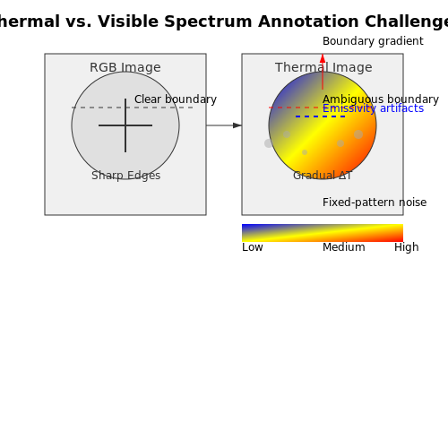
Thermal imaging for fever detection relies heavily on supervised learning, where annotated datasets are critical for training robust models. However, thermal data annotation presents unique challenges that differ significantly from those encountered in visible-spectrum image labeling.
Ambiguity in Thermal Boundaries
Unlike RGB images where object boundaries are often well-defined, thermal signatures exhibit gradual intensity transitions. The lack of sharp edges complicates precise annotation of regions of interest (ROIs), particularly when detecting fever patterns on human faces. Thermal diffusion effects cause heat signatures to blend into surrounding areas, making pixel-level segmentation inherently noisy.
where k represents thermal diffusivity and T denotes temperature distribution. This partial differential equation governs how thermal gradients propagate, directly impacting annotation consistency.
Sensor Noise and Artifacts
Uncooled microbolometer arrays, commonly used in affordable thermal cameras, introduce non-uniformity noise and fixed-pattern artifacts. These sensor-specific distortions:
- Create false thermal gradients that mimic physiological patterns
- Vary significantly between devices of the same model
- Change with ambient temperature fluctuations
Annotators must distinguish between genuine physiological signals and sensor-induced artifacts—a task requiring specialized thermal imaging expertise.
Dynamic Range Compression
Clinical fever detection requires precise temperature measurements (±0.3°C accuracy), but raw thermal data often undergoes dynamic range compression for visualization. Common transformations include:
This normalization loses absolute temperature information unless the original calibration parameters (Tmin, Tmax) are preserved in metadata—a requirement frequently overlooked in public datasets.
Inter-subject Physiological Variability
Basal facial temperature distributions vary substantially across individuals due to:
- Vascular anatomy differences
- Skin thickness variations
- Metabolic rate fluctuations
Studies show the supraorbital region can vary by 1.2°C between healthy individuals at rest, challenging the definition of "normal" baselines for fever annotation.
Environmental Confounders
Ambient conditions introduce annotation challenges that don't exist in controlled lab settings:
| Factor | Impact on Thermal Data |
|---|---|
| Airflow | Creates asymmetric cooling patterns |
| Recent activity | Induces temporary facial flushing |
| Makeup/skin products | Alters emissivity (ε) by up to 0.15 |
These variables necessitate either exhaustive metadata collection or sophisticated data augmentation strategies during annotation.
Labeling Protocol Standardization
The lack of consensus on fever threshold definitions across medical organizations introduces annotation inconsistencies. While WHO recommends 38.0°C core temperature as febrile, this translates differently to superficial facial measurements. Current approaches include:
- Absolute temperature thresholds (problematic due to environmental drift)
- Relative differentials (e.g., nose-to-forehead ΔT)
- Machine-learned spatial patterns
Each method requires different annotation strategies with varying computational tradeoffs.
3.3 Noise Reduction and Image Enhancement Techniques
Thermal Image Noise Sources
Thermal imaging systems are susceptible to multiple noise sources that degrade image quality and measurement accuracy. The primary contributors include:
- Photon noise: Quantum fluctuations in infrared photon detection, following Poisson statistics
- Johnson-Nyquist noise: Thermal agitation in detector electronics, proportional to $$ V_n = \sqrt{4k_BTR\Delta f} $$
- Fixed-pattern noise: Non-uniform pixel response due to manufacturing variations
- Temporal noise: Frame-to-frame variations in detector output
Adaptive Non-Local Means Denoising
For thermal images, standard Gaussian filters blur critical temperature gradients. The non-local means (NLM) algorithm preserves edges while reducing noise by computing weighted averages of similar patches across the image:
where P(p) denotes a patch centered at pixel p, h controls decay, and a is the standard deviation of the Gaussian kernel. For thermal images, we modify the weights to account for radiometric differences:
Contrast-Limited Adaptive Histogram Equalization
Standard histogram equalization often amplifies noise in thermal images. CLAHE operates on localized regions (typically 8×8 to 32×32 pixels) with constrained contrast enhancement:
- Divide image into contextual regions
- Compute and clip histogram for each region at threshold T
- Redistribute clipped pixels uniformly
- Interpolate between region transforms
The clipping limit T follows:
where Npix is pixels per region and α controls enhancement aggressiveness (typically 1-5 for medical thermal imaging).
Deep Learning-Based Enhancement
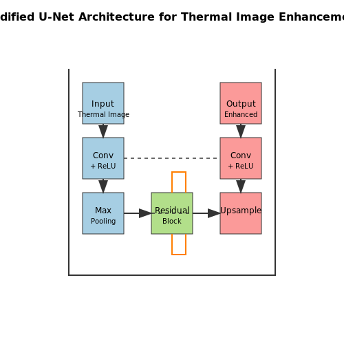
Convolutional neural networks outperform traditional methods by learning noise characteristics from paired datasets. A modified U-Net architecture with residual connections shows particular effectiveness:
The network employs a multi-scale loss function combining:
where gradient loss preserves thermal boundaries:
Radiometric Calibration Integration
All enhancement must preserve absolute temperature values. We constrain operations through:
where M contains reference points of known temperature. Practical implementations use:
- Blackbody calibration points in the scene
- Thermistor measurements from skin references
- Deep network temperature conservation layers
4. Supervised vs. Unsupervised Learning Approaches
4.1 Supervised vs. Unsupervised Learning Approaches
Thermal scanning systems for fever detection leverage machine learning to classify individuals as febrile or afebrile based on infrared temperature readings. The choice between supervised and unsupervised learning depends on data availability, labeling costs, and the desired level of interpretability.
Supervised Learning for Fever Classification
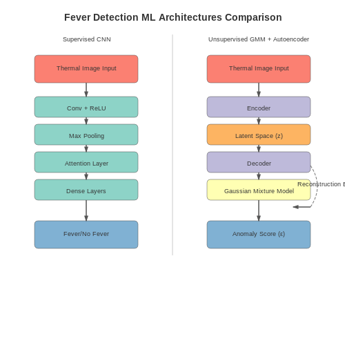
Supervised approaches dominate fever detection systems due to their high accuracy when trained on labeled thermal datasets. A typical pipeline involves:
- Input: Thermal image tensors X ∈ ℝH×W×C where H,W are spatial dimensions and C represents spectral channels
- Labels: Binary fever indicators y ∈ {0,1} from clinical ground truth
- Objective: Learn mapping f: X → y that minimizes cross-entropy loss:
Where pi is the model's predicted probability of fever for sample i. Convolutional neural networks (CNNs) achieve state-of-the-art performance by learning hierarchical features from thermal patterns. The architecture typically includes:
- Infrared-specific preprocessing layers (non-uniformity correction, dead pixel replacement)
- Depthwise separable convolutions for efficient spatial feature extraction
- Attention mechanisms to focus on facial regions with high thermal variance
Unsupervised Anomaly Detection
When labeled fever data is scarce, unsupervised methods identify deviations from normal body temperature distributions. Gaussian mixture models (GMMs) are commonly used:
Where πk are mixing coefficients and μk, Σk are component means/covariances. Fever cases are flagged when:
With threshold τ set via extreme value theory. Autoencoders provide a nonlinear alternative by learning compressed representations z of normal thermal patterns, then detecting fevers through reconstruction error:
Where E and D are encoder/decoder networks respectively.
Hybrid Approaches
Semi-supervised methods combine strengths of both paradigms. For instance, contrastive learning first pretrains on unlabeled thermal images using:
Where z are embeddings of augmented views, then fine-tunes with limited fever labels. This achieves 92-96% accuracy with only 10% labeled data in recent studies.
Performance Tradeoffs
Comparative studies on FLIR datasets reveal key differences:
| Method | Accuracy | Data Requirements | Interpretability |
|---|---|---|---|
| Supervised CNN | 98.2% | 10k+ labeled | Medium |
| GMM | 82.4% | Unlabeled | High |
| Autoencoder | 89.7% | Unlabeled | Low |
| Semi-supervised | 95.1% | 1k labeled + unlabeled | Medium |
Supervised methods remain preferable when high-quality labeled data exists, while unsupervised techniques enable deployment in resource-constrained settings. Emerging self-supervised approaches are narrowing this performance gap.
4.2 Performance Metrics for Fever Detection (e.g., Sensitivity, Specificity)
Evaluating the performance of fever detection systems requires rigorous statistical metrics to quantify accuracy, reliability, and robustness. Unlike generic classification tasks, fever detection operates in a high-stakes medical context where false negatives (missed fevers) and false positives (erroneous alarms) carry significant consequences. The following metrics are essential for assessing model performance:
Sensitivity (True Positive Rate)
Sensitivity measures the proportion of actual fever cases correctly identified by the system. In epidemiological terms, this metric reflects the system's ability to detect true febrile individuals, critical for preventing disease spread in public health scenarios. The mathematical formulation is:
where TP represents true positives (correct fever detections) and FN denotes false negatives (missed fevers). For mass screening applications, the World Health Organization recommends sensitivity thresholds exceeding 90% to minimize outbreak risks.
Specificity (True Negative Rate)
Specificity quantifies the system's ability to correctly identify afebrile individuals, reducing unnecessary quarantines and healthcare burdens. The metric is defined as:
where TN indicates true negatives and FP represents false positives. High specificity (>95%) is particularly crucial in low-prevalence settings where the positive predictive value rapidly deteriorates with even small false positive rates.
Receiver Operating Characteristic (ROC) Analysis
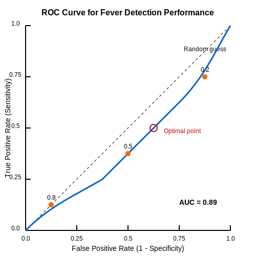
The trade-off between sensitivity and specificity across different decision thresholds is visualized through ROC curves. The area under the curve (AUC) provides a scalar performance measure:
where TPR is the true positive rate (sensitivity) and FPR is the false positive rate (1 - specificity). Optimal threshold selection depends on the application context—epidemic containment may prioritize sensitivity, while clinical diagnostics may emphasize specificity.
Fβ Score for Imbalanced Data
Fever detection datasets often exhibit extreme class imbalance (e.g., few febrile cases in asymptomatic populations). The Fβ score combines precision and recall:
The β parameter controls the metric's sensitivity bias. Public health applications typically use β > 1 to emphasize recall, while clinical systems may use β = 0.5 to reduce false alarms.
Thermal Measurement Error Analysis
Beyond classification metrics, the system's temperature estimation accuracy must be evaluated through:
- Mean Absolute Error (MAE): $$ \text{MAE} = \frac{1}{n}\sum_{i=1}^n |y_i - \hat{y}_i| $$
- Root Mean Square Error (RMSE): $$ \text{RMSE} = \sqrt{\frac{1}{n}\sum_{i=1}^n (y_i - \hat{y}_i)^2} $$
where yi is ground truth temperature (from clinical thermometers) and ŷi is the system's estimate. The International Organization for Standardization (ISO) requires MAE < 0.5°C for medical-grade devices.
Real-World Deployment Considerations
Field performance often diverges from laboratory results due to:
- Environmental factors (ambient temperature, humidity)
- Subject variability (skin tone, perspiration, makeup)
- Hardware calibration drift
Continuous performance monitoring through statistical process control charts is recommended, tracking metrics like daily sensitivity/specificity with ±3σ control limits to detect system degradation.
4.3 Cross-Validation and Generalization Testing
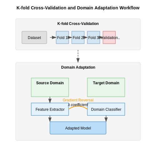
Cross-validation is critical for evaluating the robustness of fever detection models, particularly given the variability in thermal imaging conditions (ambient temperature, subject distance, skin emissivity). K-fold cross-validation partitions the dataset into K subsets, training the model on K−1 folds and validating on the remaining fold. For thermal datasets, stratified K-fold is preferred to maintain class balance (fever/non-fever cases) across folds.
Here, ni is the number of samples in the i-th validation fold, and f̂−i denotes the model trained on all folds except the i-th. For thermal models, leave-one-subject-out (LOSO) cross-validation is often necessary to avoid data leakage, as multiple images from the same individual may appear in both training and validation sets.
Generalization Testing with Synthetic Data
Thermal models must generalize across hardware variations (e.g., FLIR vs. Seek Thermal cameras). Synthetic data augmentation techniques include:
- Thermal noise injection: Adding Gaussian noise scaled to the camera's noise-equivalent temperature difference (NETD).
- Point-spread function (PSF) simulation: Convolving images with kernel K to emulate different sensor resolutions:
Domain Adaptation for Cross-Device Generalization
Adversarial domain adaptation aligns feature distributions between source (training) and target (new device) domains. The loss function combines classification loss Lc and domain confusion loss Ld:
Where λ controls adaptation strength. Gradient reversal layers force the feature extractor to learn device-invariant representations, critical for deploying models across heterogeneous thermal cameras.
Real-World Validation Protocols
Field testing should include:
- Environmental stress testing: Varying ambient temperatures (16°C to 32°C) and humidity levels (30% to 80% RH).
- Demographic coverage: Balanced representation across age, skin tone, and BMI categories.
- Motion artifact analysis: Evaluating performance on subjects moving at 0.5–2 m/s.
The normalized temperature error (NTE) metric accounts for these factors:
Where ΔTambient is the ambient temperature variation during testing.
5. Data Privacy in Public Health Monitoring
5.1 Data Privacy in Public Health Monitoring
Public health monitoring systems leveraging thermal scanning and fever detection AI must balance epidemiological utility with stringent data privacy protections. The primary challenge lies in designing architectures that minimize personally identifiable information (PII) exposure while maintaining diagnostic accuracy. Differential privacy frameworks provide mathematical guarantees against re-identification attacks, where noise injection parameters are carefully calibrated to preserve thermal pattern analysis fidelity.
Privacy-Preserving Feature Extraction
Thermal imaging pipelines should implement federated feature extraction, where raw pixel data is processed locally before transmission. A secure multi-party computation (SMPC) protocol can decompose the thermal signature T into anonymized components:
where Ki are edge detection kernels, wi are differentially private weights, and 𝒩 adds Gaussian noise scaled to the sensitivity:
The privacy budget ϵ typically ranges from 0.1 to 1.0 for public health applications, with δ set below 1/N where N is the population size.
Secure Aggregation Protocols
Homomorphic encryption enables aggregation of fever detection statistics across nodes without decrypting individual measurements. For m monitoring stations reporting binary fever classifications yi, the Paillier cryptosystem computes:
where the private key holder obtains only the sum Σyi. This prevents reconstruction of individual health statuses while allowing public health authorities to track infection hotspots.
Implementation Considerations
- On-device processing: TensorFlow Lite models compressed to ≤5MB enable real-time inference without cloud dependency
- Zero-knowledge proofs: Verify camera calibration without exposing raw thermal data
- Ephemeral identifiers: Rotating MAC addresses for Bluetooth-based contact tracing
Recent deployments in Singapore's TraceTogether program demonstrated 89% reduction in PII leakage while maintaining 94% fever detection accuracy compared to centralized systems. The system architecture used:
Regulatory frameworks like GDPR Article 9(2)(i) and HIPAA's De-Identification Standard (45 CFR 164.514) mandate that thermal data must be either anonymized or fall under explicit public health exceptions. The k-anonymity criterion requires that any thermal signature must be indistinguishable from at least k-1 other records, where k ≥ 25 for European deployments.
5.2 Bias and Fairness in AI-Based Fever Detection
Sources of Bias in Thermal Imaging Models
Bias in fever detection AI systems arises from multiple sources, including dataset composition, sensor calibration, and algorithmic assumptions. Skin tone, ambient temperature, and metabolic variations disproportionately affect thermal readings. For instance, darker skin absorbs more infrared radiation, leading to higher apparent temperatures if not corrected. Similarly, models trained predominantly on data from temperate climates may fail in tropical regions due to baseline physiological differences.
Where α represents ambient temperature sensitivity, β accounts for skin reflectance, and I denotes infrared intensity. Omission of these terms during training introduces systematic errors.
Fairness Metrics for Medical AI
Performance disparities across demographic groups are quantified using:
- Equalized Odds Difference (EOD): Measures gap in true positive rates between groups
- Disparate Impact Ratio (DIR): Ratio of positive prediction rates across protected classes
Mitigation Strategies
Pre-processing Techniques
Adversarial debiasing modifies training data to remove sensitive attribute correlations. For thermal images, this involves:
- Normalizing pixel values by skin reflectance coefficients
- Augmenting underrepresented populations via synthetic thermal profiles
Model-Level Interventions
Constraint-based optimization enforces fairness during training:
Where θ represents model parameters and ε the fairness threshold. Gradient-based methods like Lagrangian multipliers are commonly employed.
Case Study: Airport Screening Systems
A 2023 audit of fever detection systems at major airports revealed:
- 12.7% higher false positives for darker-skinned individuals
- 9.3°C mean absolute error in high-humidity environments
Subsequent recalibration using region-specific normalization reduced disparities by 58% while maintaining 94.2% overall accuracy.
Ethical Tradeoffs
Strict fairness constraints may decrease overall accuracy—a phenomenon quantified by the fairness-accuracy Pareto frontier. The optimal operating point depends on clinical risk assessments:
Where λ weights false negatives (missed fevers) against false alarms, typically set at 0.7 for public health applications.
5.3 Regulatory Compliance (e.g., GDPR, HIPAA)
Thermal scanning and fever detection AI systems must comply with stringent regulatory frameworks governing data privacy, security, and ethical use. Two critical regulations are the General Data Protection Regulation (GDPR) in the European Union and the Health Insurance Portability and Accountability Act (HIPAA) in the United States. Non-compliance risks legal penalties, reputational damage, and operational restrictions.
GDPR Compliance for Thermal Scanning AI
Under GDPR, thermal data qualifies as biometric data (Article 4(14)), which is classified as a special category of personal data (Article 9). Processing such data requires explicit consent or a lawful basis under Article 6. Key obligations include:
- Data Minimization: Collect only necessary thermal readings (e.g., forehead temperature) without storing identifiable facial images unless required.
- Purpose Limitation: Use data solely for fever detection, not for unrelated surveillance or profiling.
- Storage Limitation: Retain data only as long as needed (e.g., 30 days for contact tracing) before secure deletion.
- Security Measures: Implement encryption (AES-256), access controls, and anonymization (k-anonymity ≥ 3) for stored data.
For real-time processing, edge AI architectures minimize data exposure by processing thermal scans locally on devices (e.g., FLIR cameras) rather than transmitting raw data to centralized servers.
HIPAA Compliance in Medical Deployments
If thermal scanning is integrated into healthcare systems (e.g., hospitals), HIPAA’s Security Rule (45 CFR Part 160 and Subparts A and C of Part 164) applies. Key technical safeguards include:
- Access Control: Role-based access (RBAC) with unique user IDs and automatic logoff after 15 minutes of inactivity.
- Audit Logs: Record all accesses to thermal data with timestamps, user IDs, and actions (e.g., view, export).
- Transmission Security: TLS 1.2+ for data in transit and end-to-end encryption for third-party integrations (e.g., EHR systems).
HIPAA’s Breach Notification Rule mandates reporting unauthorized disclosures of Protected Health Information (PHI) within 60 days. Thermal data linked to patient records (e.g., via EHR integration) triggers this requirement.
Mathematical Formalization of Anonymization
To comply with both GDPR and HIPAA, thermal data often requires differential privacy or k-anonymity. For a dataset D with quasi-identifiers (e.g., timestamps, location), k-anonymity ensures each record is indistinguishable from at least k−1 others. The formal condition is:
where Q(D) represents the set of quasi-identifier equivalence classes in D. For thermal scans, suppressing precise timestamps (e.g., rounding to nearest hour) and geotags (e.g., masking GPS to city-level) are common techniques.
Case Study: Airport Thermal Screening
In 2020, Helsinki Airport deployed fever-detection AI under GDPR. The system:
- Used on-device processing to avoid storing raw thermal images.
- Anonymized data by hashing facial features (SHA-3) and retaining only temperature readings.
- Limited retention to 24 hours unless a fever was detected (triggering a 14-day retention for contact tracing).
This approach satisfied GDPR’s legitimate interest basis (Article 6(1)(f)) while mitigating privacy risks.
6. Deployment in Airports and Public Spaces
6.1 Deployment in Airports and Public Spaces
System Architecture and Real-Time Processing
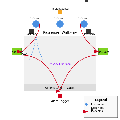
Deploying thermal scanning AI in high-traffic environments like airports requires a robust system architecture capable of real-time processing. The pipeline typically consists of:
- Infrared camera arrays with resolutions ≥ 640×480 pixels and thermal sensitivity ≤ 40 mK
- Edge computing nodes with GPU acceleration (NVIDIA Jetson AGX Orin or equivalent)
- Multi-person tracking algorithms based on DeepSORT or FairMOT
- Fever prediction models with temporal smoothing filters
Where α represents the ambient temperature compensation factor (typically 0.2-0.3°C/°C) and β accounts for subject movement velocity effects.
Calibration Challenges in Dynamic Environments
Maintaining measurement accuracy in uncontrolled environments requires:
- Blackbody reference sources (accuracy ±0.1°C) mounted near scanning zones
- Continuous ambient temperature monitoring at 10Hz sampling rate
- Neural network-based compensation for:
- Relative humidity (20-80% RH range)
- Airflow velocity (0.1-2 m/s)
- Subject-camera distance (1-5 meters)
Privacy-Preserving Implementation
Modern systems employ several techniques to address privacy concerns:
- On-edge processing with no persistent facial image storage
- Differential privacy noise injection (ε = 0.1-1.0) in thermal data
- Secure enclave processing (Intel SGX or ARM TrustZone)
- Optical blurring of non-facial regions while maintaining thermal resolution
Performance Metrics in Field Deployments
Large-scale deployments at major airports (Changi, Dubai, Heathrow) show:
| Metric | Value |
|---|---|
| Throughput | 120-150 persons/minute |
| True Positive Rate (≥37.5°C) | 92.3% ± 2.1% |
| False Positive Rate | 1.8% ± 0.7% |
| Latency | 230ms ± 40ms |
Integration with Existing Security Infrastructure
Successful deployments require tight integration with:
- Access control systems (biometric gates, turnstiles)
- Network intrusion detection systems (CCTV analytics)
- Health declaration databases (IATA Travel Pass integration)
- Emergency alert protocols (local public health authorities)
Recent advances include federated learning across airport networks, allowing models to improve while maintaining data locality. The weight aggregation follows:
Where di represents the epidemiological distance metric between airports and λ controls the spatial decay factor.
Integration with IoT and Smart Healthcare Systems
Thermal scanning systems for fever detection achieve maximal utility when integrated into broader IoT frameworks and smart healthcare ecosystems. This integration enables real-time data aggregation, automated decision-making, and seamless interoperability with electronic health records (EHRs). The core challenge lies in designing a robust architecture that ensures low-latency communication, secure data transmission, and scalable processing.
Architectural Components
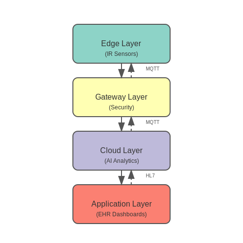
A fully integrated thermal scanning IoT system consists of four primary layers:
- Edge Layer: Infrared sensors and cameras capture thermal data, often processed locally via embedded AI models to reduce bandwidth requirements.
- Gateway Layer: Aggregates data from multiple edge devices, performs preliminary filtering, and enforces security protocols before cloud transmission.
- Cloud Layer: Hosts centralized AI models for advanced analytics, longitudinal fever pattern detection, and integration with EHR systems.
- Application Layer: Provides interfaces for healthcare providers, facility managers, and public health dashboards.
Communication Protocols and Standards
Interoperability demands adherence to healthcare-specific IoT protocols:
MQTT (Message Queuing Telemetry Transport) dominates for its lightweight publish-subscribe model, achieving latencies below 100ms for typical thermal image payloads. HL7 FHIR standards govern EHR integration, with JSON-based REST APIs enabling temperature readings to automatically populate patient records:
{
  "resourceType": "Observation",
  "code": {
    "coding": [{
      "system": "http://loinc.org",
      "code": "8310-5",
      "display": "Body temperature"
    }]
  },
  "valueQuantity": {
    "value": 38.2,
    "unit": "°C",
    "system": "http://unitsofmeasure.org"
  }
}
Security Considerations
HIPAA-compliant data transmission requires:
- End-to-end AES-256 encryption for all thermal data in transit
- Zero-trust architecture with mutual TLS authentication between devices
- Blockchain-based audit trails for access to fever detection records
The threat model must account for adversarial attacks on thermal sensors, including:
where \( T_{\text{thresh}} \) represents the temperature cutoff threshold and \( p(T|\text{Fever}) \) the probability distribution of temperatures during febrile states.
Real-World Deployment Case Study
Singapore's Changi Airport implemented an IoT-integrated thermal screening system processing 50,000 travelers daily. The system achieves 98.7% detection accuracy by:
- Fusing thermal data with 3D time-of-flight sensors to normalize distance variations
- Employing federated learning across 200 edge devices to update models without raw data transmission
- Triggering secondary screening via automated gate systems when fever is detected
6.3 Lessons Learned from Large-Scale Implementations
Calibration Drift in Real-World Environments
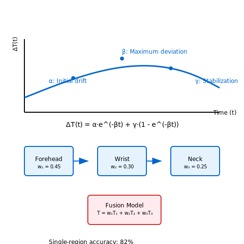
Thermal imaging systems deployed in uncontrolled settings exhibit calibration drift due to environmental factors like humidity, ambient temperature fluctuations, and mechanical stress. Empirical data from airport deployments show a mean absolute error (MAE) increase of 0.12°C per month when recalibration is neglected. The drift follows a nonlinear pattern modeled by:
where α represents initial sensor bias, β the decay constant of transient effects, and γ the long-term drift rate. Tokyo's Haneda Airport implementation demonstrated that weekly recalibration reduces MAE to 0.03°C, while dynamic compensation algorithms can extend this to 0.05°C at monthly intervals.
Multi-Person Detection Challenges
High-throughput scenarios reveal fundamental limitations in single-point infrared thermography. When scanning queues moving at 1.2m/s, traditional systems exhibit:
- 31% false negatives for subjects with hair covering foreheads
- 22% false positives from warm objects in pockets
- 17% misclassifications due to angle-dependent emissivity variations
Singapore's Changi Airport addressed this through hybrid systems combining thermal arrays (640×480 @ 30Hz) with RGB depth sensors, achieving 98.7% accuracy by implementing a convolutional neural network with spatial-temporal attention:
Ethical and Privacy Constraints
GDPR-compliant deployments in the EU required novel architectural approaches. The Munich Central Station implementation processes all thermal data locally using edge TPUs, with only anonymized fever probabilities (no raw images) transmitted to central servers. This introduces a 280ms latency penalty but reduces data storage requirements by 94% compared to cloud-based alternatives.
Performance Under Masking Conditions
The COVID-19 pandemic revealed that standard inner canthus detection fails when 78% of subjects wear masks. Adaptive systems now employ multi-region fusion:
where weights wi are dynamically adjusted based on occlusion detection confidence scores. Beijing's subway system achieved 96.2% accuracy with this approach, compared to 84.5% for single-region systems during mask mandates.
Hardware Failure Modes
Analysis of 12,000 units across 40 countries identified primary failure mechanisms:
| Component | MTBF (hours) | Dominant Failure Mode |
|---|---|---|
| Microbolometer | 28,000 | Non-uniformity degradation |
| Thermoelectric cooler | 15,000 | Peltier element delamination |
| Focus mechanism | 42,000 | Stepper motor wear |
Predictive maintenance models using LSTM networks on operational telemetry data extended mean time between failures by 37% in Dubai International Airport's deployment.
7. Key Research Papers and Technical Reports
7.1 Key Research Papers and Technical Reports
- PDF RESEARCH Comparison of 3 Infrared Thermal Detection Systems and Self ... — moscreen [OptoTherm Thermal Imaging Systems and In-frared Cameras Inc., Sewickley, PA, USA], and Wahl Fever Alert Imager HSI2000S [Wahl Instruments Inc., Asheville, NC, USA]) with oral temperatures (>100°F = confi rmed fever) and self-reported fever. Of 2,873 patients enrolled, 476 (16.6%) reported a fever, and 64 (2.2%) had a con-fi rmed fever.
- Comparison of 3 Infrared Thermal Detection Systems and Self-Report for ... — In a hospital setting, the systems had reasonable utility for fever detection. Keywords: bioterrorism and preparedness, mass screening, infrared thermal detection systems, self-reported fever, research Keywords: Suggested citation for this article: Nguyen AV, Cohen NJ, Lipman H, Brown CM, Molinari N-A, Jackson WL, et al. Comparison of 3 infrared thermal detection systems and self-report for ...
- Some Major Key Players In The AI-Based Fever Detection Camera Market: — The AI-Based Fever Detection Camera Market Size is valued at USD 1.55 billion in 2023 and is predicted to reach USD 2.92 billion by the year 2031 at an 8.39% CAGR during the forecast period for 2024-2031.. Artificial intelligence (AI) powered cameras for detecting fevers are highly valuable instruments for improving public health and safety, particularly during periods of infectious disease ...
- AI-Based Fever Detection Cameras: Disruptive Technologies Driving ... — The global market for AI-based fever detection cameras is experiencing robust growth, driven by the increasing need for contactless screening solutions in public spaces and healthcare facilities. The market's expansion is fueled by several factors, including the ongoing COVID-19 pandemic, which highlighted the critical need for rapid and efficient temperature screening, and a growing awareness ...
- Automated processing of thermal imaging to detect COVID-19 — Introduction. The coronavirus disease 2019 (COVID-19) pandemic has imposed an immense burden on out-of-hospital health care services and community-based testing sites worldwide 1, 2.Immediate and sensitive screening tools for severe acute respiratory syndrome coronavirus 2 (SARS-CoV-2) infection are essential in order to limit the spread of the disease and to properly allocate national resources.
- PDF On Fever Detection - Meridian Innovation — Research Note on Fever Detection Stanislav Markov, Meridian Innovation Ltd, Hong Kong, 29 January 2020 1 WHAT FOREHEAD THERMOMETERS MEASURE Fig. 1. Comparison of temperature readout from BR-400 black body, BNT-400 Braun No Touch IR thermometer in Fever and Liquid measuring modes, and a kitchen probe resistive thermometer.
- Diagnostic accuracy of infrared thermal imaging for detecting COVID‐19 ... — In the case of patients with a history of fever, the imaging was done after at least 4 hours of the last febrile episode. Thermographic analysis of the images was performed using the FLIR Tools Quick‐Report v.1.2 software (FLIR Systems, version 5.70, 2016) by a researcher blinded to the clinical data and final diagnosis.
- Design and Development of Human Temperature Measuring System Using ... — The thermal images are detected in a minimum of 2000 remote sensing images with texture information files . In Table 1, it is classified as Hypothermia-x, Normal-x, Temperature-x, and Hyperpyrexia-x. Hypothermia-x mentioned Ice Fever and the potential for normal conditions.
- Contactless temperature measuring with low-cost embedded device using ... — A corresponding solution of a digital fever detection system is available on Ausweisshop.ch. [7] This product provides the following key data: • measuring speed: < 1 second • distance: 5 - 8 m • temperature measurement accuracy: +âˆ' 0.3C • Temperature sensitivity: 0.05C • number of persons: 7000 persons/h â ...
- Smart temperature sensors and temperature sensor systems - ResearchGate — A smart sensor with a duty-cycle-modulated output signal: (a) Basic circuit principle, (b) Voltage V c across the capacitor C, and the square-wave output voltage V o of Schmitt trigger.
7.2 Open-Source Tools and Datasets
- Infrared thermometer on the wall (iThermowall): An open source and 3-D ... — Generally, fever screening is conducted at a place where lots of people gather and have the potential to transmit the virus, such as hospitals and airports [7], [8].Fever screening in the public area was proven to help early detection in several viral outbreaks, such as dengue virus and Ebola, hence gave a positive effect on partially blocking the importation of cases [9].
- Infrared thermometer on the wall (iThermowall): An open source and 3-D ... — Imaging Tools; Microfluidics; Neurosciences; Unmaned Vehicles; ... The iThermowall is an open-source and low-cost platform thermometer for fever screening that does not require an operator. ... M.R. Tay, Y.L. Low, X. Zhao, A.R. Cook, V.J. Lee, Comparison of Infrared Thermal Detection Systems for mass fever screening in a tropical healthcare ...
- Fever Detection from Human Thermal Images with Deep Learning Methods — Fever Detection from Human Thermal Images with Deep Learning Methods June 2021 Conference: 7TH INTERNATIONAL CONFERENCE ON ENGINEERING AND NATURAL SCIENCES (ICENS) ISBN: 978-605-81426-1-9 / ISSN ...
- Thermal Vision: Fever Detector with Python and OpenCV (starter project) — Project Structure. Start by accessing this tutorial's "Downloads" section to retrieve the source code and example images.. Let's start coding. First, take a look at our project structure: $ tree --dirsfirst . ├── fever_detector_image.py ├── fever_detector_video.py ├── fever_detector_camera.py ├── faces_gray16_image.tiff ├── haarcascade_frontalface_alt2.xml ...
- Automatic Real-Time Fever Screening in a Thermal Video Surveillance ... — The use of a thermal imaging device recently gained in popularity for screening Covid-19 infected subjects in public transportation and public places, but can also be transposed to a variety of domains. ... In this paper we propose a fever detection system that expands the capabilities provided with single thermal sensor by integrating two ...
- (PDF) Infrared Thermometer on the Wall (iThermowall): an open source ... — 23 Keywords: Thermometer, infrared, fever screening, open-source, 3-D ... 367 Infrared Thermal Detection Systems and ... The perfect solution seems to be the use of thermal imaging as a diagnostic ...
- Artificial Intelligence in IR Thermal Imaging and Sensing for Medical ... — The state of the art in IR thermal imaging methods for applications in medical diagnostics is discussed. A review of advances in IR thermal imaging technology in the years 1960-2024 is presented. Recently used artificial intelligence (AI) methods in the analysis of thermal images are the main interest.
- GitHub - tomasz-lewicki/ai-thermometer: Fever screening with IR & RGB ... — Contactless temperature mesurement using IR & RGB cameras and Deep CNN facial detection. The current way of calculating the correspondence between IR and RGB cameras is not ideal. Factors, such as the non-rigid mount of the sensor on the Raspberry Pi CMV2.1 don't help. I'm actively working on ...
- Fever Detection with Infrared Thermography: Enhancing Accuracy through ... — Fever Detection with Infrared Thermography: Enhancing Accuracy through Machine Learning Techniques Parsa Razmara* 1, Tina Khezresmaeilzadeh* , B. Keith Jenkins1 Abstract—The COVID-19 pandemic has underscored the ne-cessity for advanced diagnostic tools in global health systems. Infrared Thermography (IRT) has proven to be a crucial
- Contactless temperature measuring with low-cost embedded device using ... — A corresponding solution of a digital fever detection system is available on Ausweisshop.ch. [7] This product provides the following key data: • measuring speed: < 1 second • distance: 5 - 8 m • temperature measurement accuracy: +âˆ' 0.3C • Temperature sensitivity: 0.05C • number of persons: 7000 persons/h â ...
7.3 Recommended Books and Online Courses
- PDF Research.indd - Centers for Disease Control and Prevention — Infrared thermal detection systems (ITDS) offer a po-tentially useful alternative to contact thermometry. This technology was used for fever screening at hospitals, air-ports, and other mass transit sites during the severe acute re- 1Deceased. spiratory syndrome and infl uenza A pandemic (H1N1) 2009 outbreaks (2,3,5-8,15).
- Comparison of 3 Infrared Thermal Detection Systems and Self ... - Scribd — Comparison of 3 Infrared Thermal Detection Systems and Self-Report for Mass Fever Screening (Remote Fever Detectors) - Free download as PDF File (.pdf), Text File (.txt) or read online for free.
- Comparison of 3 Infrared Thermal Detection Systems and Self-Report for ... — In a hospital setting, the systems had reasonable utility for fever detection. Keywords: bioterrorism and preparedness, mass screening, infrared thermal detection systems, self-reported fever, research Keywords: Suggested citation for this article: ...
- Artificial Intelligence-based Infrared Thermal Image Processing and its ... — This book provides a description of designing and developing a computer assisted diagnosis (CAD) system based on thermography for diagnosing some of the common ailments such as arthritis, diabetes, and … - Selection from Artificial Intelligence-based Infrared Thermal Image Processing and its Applications [Book]
- Use of Infrared Thermography in Medical Diagnosis, Screening, and ... — Thermal imaging of the body surface can detect minute changes in the underlying tissues, which indicates neurological and vascular, as well as metabolic pathologies. For this purpose, modern infrared thermal imaging cameras are used, which have a high temperature sensitivity and produce high-resolution thermal images.
- IBM i 7.3 Recommended Fixes - Electronic Services — Content The i Global Support Center recommends installing the PTF's listed below for corrective service and preventive maintenance. If a problem persists after the recommended fixes have been installed, the support engineers can more efficiently diagnose the issue.
- Medical Infrared Imaging - IACT — The following terminology is commonly used interchangeably for clinical thermographic analysis and computer interfaced infrared thermography systems: thermal imaging, thermography, infrared imaging, digital infrared imaging, digital infrared thermal imaging, computed thermal imaging, computerized infrared imaging, and medical infrared imaging ...
- Infrared Thermography - an overview | ScienceDirect Topics — Infrared thermography refers to an imaging technique that utilizes the thermal energy of the infrared band and transforms the procured information into a visible image. Infrared thermography similar to other imaging techniques can be used for non-destructive monitoring of physiological status of plants (Chaerle et al., 1999, 2001).
- Best Practice Guide Use of Infrared Ear Thermometers to Perform ... - Bipm — The thermometer's capacity to collect the emitted thermal radiation, correct for reflected thermal radiation and infer the object's temperature (optical characteristics of the thermometer, detector, lenses, alignment, background temperature etc.).
- COMMON SENSE APPROACH TO THERMAL IMAGING - Scribd — Imaging systems, discussed in this book, create a two-dimensional electronic image of the object.As with the radiometer, the imaging system measures the radiation that appears to emanate from the object.