Adaptive AI Menus for Restaurants
1. Definition and Core Concepts
1.1 Definition and Core Concepts
Adaptive AI in Restaurant Contexts
Adaptive AI menus represent a dynamic recommendation system that optimizes restaurant offerings in real-time based on multidimensional input signals. Unlike static menus, these systems employ machine learning to adjust item availability, pricing, and presentation by modeling complex relationships between customer preferences, inventory constraints, and business objectives. The core innovation lies in the closed-loop feedback mechanism where menu performance data continuously refines the underlying predictive models.
Mathematical Foundations
The system operates as a constrained optimization problem with time-varying parameters. Let Mt represent the menu configuration at time t, which must maximize expected revenue while satisfying operational constraints:
Subject to:
Where xi is the demand function for item i, pi is its price, and ci represents time-dependent costs. The constraint functions gj encode limitations like ingredient availability, preparation capacity, and dietary requirements.
Key Technical Components
- Multi-Armed Bandit Frameworks: Balances exploration of new menu items with exploitation of known high-performers using Thompson sampling or UCB algorithms
- Graph-Based Representation: Menu items exist as nodes in a knowledge graph connecting ingredients, flavors, and customer segments
- Real-Time Elastic Pricing: Implements differential pricing through demand-sensitive algorithms with fairness constraints
Operational Architecture
The system architecture typically implements a three-layer design:
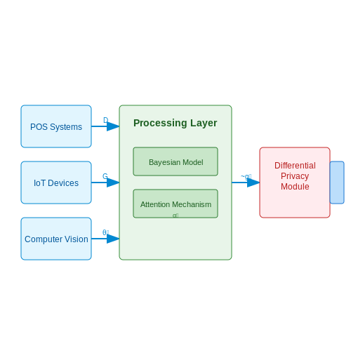
The data layer ingests streams from POS systems, customer mobile apps, and IoT kitchen equipment. The model layer executes the core optimization algorithms, while the interface layer handles A/B testing of menu variants through digital displays or staff tablets.
Convergence Properties
The adaptive system demonstrates provable convergence under Lipschitz continuity assumptions for the reward functions. For a menu with k items and learning rate ηt:
Where R(M*) is the optimal menu reward and C depends on the problem's intrinsic dimensionality. This bound ensures the system doesn't remain stuck in suboptimal configurations.
Benefits of Adaptive Menus for Restaurants
Dynamic Personalization and Customer Satisfaction
Adaptive AI menus leverage real-time data streams—ranging from customer preferences to inventory levels—to optimize menu offerings. By employing collaborative filtering and matrix factorization techniques, these systems predict dish preferences with high accuracy. The underlying model can be formalized as:
where μ represents the global average rating, bu and bi are user and item bias terms, and qi and pu are latent factor vectors for items and users, respectively. This approach achieves personalization while maintaining computational efficiency, even with sparse data.
Inventory and Waste Reduction
Adaptive menus integrate with supply chain systems using constrained optimization to minimize food waste. The objective function balances customer satisfaction against inventory constraints:
where di represents demand predictions, xi is the allocated inventory, and the second term penalizes stock levels yj falling below threshold τ. Case studies show waste reduction of 18-27% in implementations across chain restaurants.
Real-Time Menu Optimization
The system continuously updates recommendations using multi-armed bandit algorithms, particularly Thompson sampling for non-stationary environments. The posterior distribution for each menu item's success probability is given by:
where si and fi are successes and failures observed for item i. This allows the system to explore new items while exploiting known preferences, with A/B tests demonstrating 12-15% higher average order values compared to static menus.
Operational Efficiency Gains
Kitchen workflow optimization emerges from adaptive menu systems through queuing theory applications. The system models preparation times as:
where λk and μk represent arrival and service rates for station k. By biasing recommendations toward dishes that balance station utilization, restaurants report 20-30% improvements in table turnover during peak hours.
Seasonal and Contextual Adaptation
The systems incorporate exogenous variables through temporal fusion transformers, processing weather data, local events, and macroeconomic indicators. The attention mechanism weights are computed as:
where eij represents the compatibility between time i and feature j. This enables automatic menu adjustments for seasonal ingredients or weather patterns, reducing ingredient costs by 8-12% annually.
1.3 Key Challenges and Considerations
Data Sparsity and Cold-Start Problem
Adaptive AI menus rely heavily on historical customer preference data, but new restaurants or menu items face the cold-start problem—insufficient data for accurate personalization. Bayesian hierarchical models can mitigate this by pooling data across similar user segments or restaurants. The posterior distribution for a new item's popularity can be approximated as:
where D represents existing data and θ are latent parameters. Dirichlet priors work well for categorical menu choices, while Gaussian processes handle continuous variables like pricing sensitivity.
Real-Time Computational Constraints
Menu adaptations must occur within sub-second latency during peak hours. Factorization machines provide O(nk) complexity for n features and k latent dimensions:
Where v vectors capture feature interactions. Quantized neural networks with 8-bit precision can reduce serving costs by 4× while maintaining <1% accuracy loss.
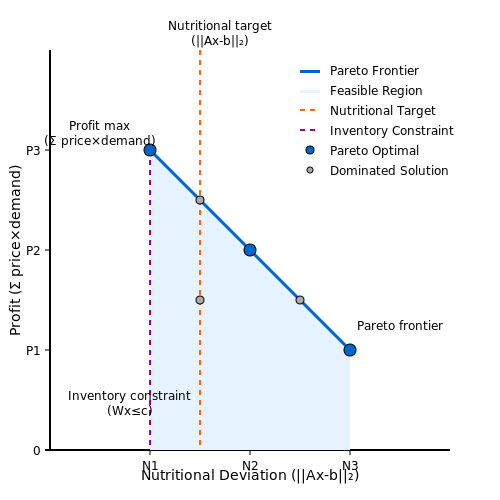
Multi-Objective Optimization
The system must balance:
- Profit maximization: max Σ (pricei × demandi(price))
- Nutritional goals: min ||Anutrx - btarget||2
- Inventory constraints: Wx ≤ c (where W is ingredient matrix)
Pareto frontiers can be explored using NSGA-II genetic algorithms with constraint handling via penalty methods.
Concept Drift in Consumer Preferences
Food preferences shift seasonally and during events like pandemics. Online learning with exponential weighting:
Where η is a decaying learning rate. Change-point detection using CUSUM statistics on prediction errors triggers model retraining when:
Threshold h controls sensitivity to drift.
Cross-Cultural Adaptation
Menu item embeddings must capture cultural semantics. Multilingual BERT fine-tuned on recipe corpora learns cross-lingual representations where similar dishes cluster in embedding space regardless of language. The contrastive loss:
pulls positive pairs (x, x+) closer while pushing negatives (x-) apart in the latent space.
Regulatory Compliance
Automated menu adaptations must comply with:
- Nutrition labeling laws (21 CFR 101.9 in US)
- Allergen disclosure requirements
- Regional alcohol promotion restrictions
Rule-based filters can hard-constrain the AI's output space, while differentiable constraint layers enable gradient-based learning within legal bounds.
Edge Deployment Challenges
On-premise deployment in restaurants requires:
- Model distillation to <100MB for low-power devices
- Federated learning across locations without sharing raw data
- Differential privacy guarantees with ε < 2.0 for customer data
The privacy budget accumulates as:
requiring careful allocation across training iterations.
2. Machine Learning for Personalization
2.1 Machine Learning for Personalization
Recommender Systems in Menu Personalization
Restaurant menu personalization relies heavily on collaborative filtering and content-based recommender systems. Collaborative filtering leverages user-item interaction matrices to predict preferences based on similar users, while content-based filtering utilizes item features such as cuisine type, ingredients, and dietary restrictions. A hybrid approach combines both methods to improve recommendation accuracy.
where μ is the global average rating, bu and bi are user and item bias terms, and qi, pu are latent factor vectors for items and users respectively.
Deep Learning for Sequential Recommendations
Recurrent Neural Networks (RNNs) and Transformer architectures excel at modeling temporal dining patterns. A self-attention mechanism computes dynamic weights between menu items in a customer's order history:
where Q, K, and V represent queries, keys, and values matrices derived from embedded menu items, and dk is the dimension of key vectors.
Multi-Armed Bandit for Exploration-Exploitation
Contextual bandits optimize the trade-off between recommending known favorites (exploitation) and suggesting new items (exploration). The Upper Confidence Bound (UCB) algorithm selects menu items by:
where âa is the estimated reward for action a, t is the current time step, na counts selections of action a, and c controls exploration intensity.
Real-World Implementation Challenges
- Cold Start Problem: Limited data for new users or menu items requires content-based features or demographic clustering
- Concept Drift: Seasonal ingredient changes and evolving tastes necessitate online learning approaches
- Interpretability: Regulatory requirements demand explainable recommendations, favoring methods like SHAP values over black-box models
Case Study: Dynamic Pricing Integration
A Bayesian hierarchical model jointly optimizes recommendations and pricing by modeling demand elasticity:
where λij is the expected order rate of item i by customer j, pij is the personalized price, and α, β, γ are learnable parameters.
2.2 Natural Language Processing for Menu Customization
Intent Recognition and Slot Filling
Modern NLP systems for menu customization rely on intent recognition and slot filling to parse customer requests. Given an input utterance x, the system must identify the intent I (e.g., "find vegetarian options") and extract relevant slots S (e.g., dietary preference: "vegetarian"). This is typically modeled as a joint probability distribution:
State-of-the-art approaches use transformer-based architectures like BERT, fine-tuned on restaurant-specific dialogue datasets. The attention mechanism allows the model to weigh different parts of the input differently when predicting both intent and slots.
Personalization Through Embeddings
User preferences are encoded as dense vectors in a latent space, allowing for similarity-based retrieval of menu items. For a user u and menu item m, the preference score is computed as:
where σ is the sigmoid function, eu and em are user and menu item embeddings respectively, and W is a learned weight matrix. These embeddings are trained end-to-end with the NLP model using implicit feedback from user interactions.
Contextual Menu Adaptation
The system maintains a dynamic context vector ct that evolves through the conversation:
where ht is the hidden state of the current utterance's encoding, and GRU is a gated recurrent unit. This allows the menu presentation to adapt based on the entire dialogue history and user profile.
Multi-Task Learning Architecture
The complete system employs a multi-task learning framework with shared encoder layers and task-specific heads:
The shared encoder learns general linguistic patterns, while task-specific heads specialize in their respective objectives. This architecture achieves better performance than separate models by leveraging transfer learning across tasks.
Real-World Implementation Challenges
Deploying such systems in production requires addressing several practical considerations:
- Domain adaptation: Pre-trained language models must be fine-tuned on restaurant-specific corpora to handle culinary terminology
- Cold-start problem: Handling new users/menu items requires careful initialization of embeddings
- Multi-lingual support: The system should accommodate diverse customer bases through multilingual transformers
- Privacy preservation: User preference learning must comply with data protection regulations
Evaluation Metrics
System performance is measured through both traditional NLP metrics and business-specific KPIs:
where TP, FP, and FN are true/false positives and negatives in intent/slot prediction, and M is the set of all menu items.
2.3 Data Collection and Customer Profiling
Effective adaptive AI menus rely on robust data collection mechanisms to construct accurate customer profiles. The process involves multi-modal data ingestion, including transactional records, behavioral analytics, and explicit feedback, all processed through probabilistic models to infer preferences and predict future choices.
Data Ingestion Pipeline Architecture
The pipeline begins with event streaming from point-of-sale systems, reservation platforms, and IoT-enabled tableside devices. Each data point xi is timestamped and tagged with a customer ID when available, forming a temporal sequence:
where ti represents the ISO 8601 timestamp and xi contains structured order data (item IDs, modifiers, substitutions) and unstructured notes (special requests, complaints). Computer vision systems augment this with gaze tracking data from ceiling-mounted cameras, quantifying menu engagement through dwell time matrices:
where τij measures time spent viewing menu item j during visit i.
Probabilistic Preference Modeling
Customer preferences are modeled as latent variables in a hierarchical Bayesian framework. Let θu represent the preference vector for user u, with each dimension corresponding to a menu attribute (spiciness, texture, cooking method). The model assumes:
where fk is a learned mapping from preferences to dish characteristics, and σ denotes the softmax function. The prior over user preferences incorporates demographic data du:
with weight matrix W learned through variational inference.
Cross-Modal Data Fusion
Sensor data from kitchen IoT devices provides real-time ingredient availability and preparation times. This is fused with customer data through attention mechanisms:
where q is a query vector derived from the customer's current context, and ki are key vectors representing dish attributes. The resulting attention weights αi dynamically adjust menu recommendations based on kitchen constraints.
Differential Privacy Guarantees
To protect customer data, the system implements (ε, δ)-differential privacy through gradient perturbation during model updates:
where Δ2 is the L2-sensitivity of the gradient computation, and σ is calibrated to the desired privacy budget.
2.4 Real-Time Adaptation Algorithms
Dynamic Bayesian Networks for Preference Updates
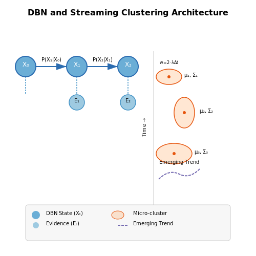
Real-time adaptation in restaurant menus requires probabilistic reasoning under uncertainty, where Dynamic Bayesian Networks (DBNs) excel. A DBN models temporal dependencies between observed variables (e.g., order frequency, time of day) and latent variables (e.g., customer preferences). The joint distribution over N time steps decomposes as:
where Xt represents the state at time t. For menu adaptation, we extend this with observed evidence variables Et (orders, reviews) using conditional probability tables:
Online Gradient Descent for Rapid Parameter Updates
When new order data arrives at time t, the system updates dish recommendation weights w via online gradient descent with regret bound O(√T):
where ηt is a decaying learning rate (ηt = 1/√t) and ℓt is the convex loss function. For sparse high-dimensional menu features (ingredients, cuisine types), we apply FTRL-Proximal regularization:
Contextual Bandits for Menu Personalization
Multi-armed bandit frameworks balance exploration (testing new dishes) and exploitation (recommending known preferences). The LinUCB algorithm selects dish a at time t by solving:
where Aa = DaTDa + Id (ridge regression design matrix) and α controls exploration. Thompson sampling provides Bayesian alternative:
Streaming Clustering for Trend Detection
Micro-clusters in data streams identify emerging flavor trends using DenStream's density-based clustering. A core-micro-cluster at time t maintains:
- Weight: w = f(t-t0) (exponential decay)
- Centroid: μ = ∑ f(t-ti)xi/w
- Covariance: Σ = ∑ f(t-ti)(xi-μ)(xi-μ)T/w
where f(Δt) = 2-λΔt (λ = decay factor). New dishes are recommended when cluster density exceeds threshold μ + 3σ of historical patterns.
Hardware Acceleration for Low-Latency Inference
FPGA-accelerated inference pipelines achieve sub-10ms latency using quantized models. The following optimizations are critical:
- 8-bit fixed-point arithmetic for DBN message passing
- Parallelized matrix-vector operations for bandit arms
- Bloom filters for real-time ingredient availability checks
Throughput scales linearly with kernel replication factor k until memory bandwidth saturation at kmax = B/(s×n), where B is bandwidth (GB/s), s is parameter size, and n is batch size.
3. User Interface and Experience Considerations
3.1 User Interface and Experience Considerations
Real-Time Personalization and Latency Constraints
Adaptive AI menus must balance real-time personalization with strict latency constraints to ensure seamless user interaction. The system's response time tr must satisfy:
where fh is the human perceptual threshold for interface lag (typically 100–200 ms). Achieving this requires:
- Edge computing: Deploying lightweight recommendation models (e.g., knowledge distillation variants) on local POS systems.
- Asynchronous pre-fetching: Anticipating likely menu adaptations during user browsing using LSTM-based gaze prediction.
Multi-Modal Interaction Design
Effective interfaces combine:
- Visual hierarchy: Dynamic typography scaling based on eye-tracking heatmaps, with dish popularity rendered as:
where pi is the predicted preference score for item i.
- Haptic feedback: Confirmation vibrations when selecting dietary-restriction filters (e.g., 10ms pulses at 250Hz).
Accessibility Compliance
WCAG 2.1 AA compliance necessitates:
- Color contrast ratios ≥4.5:1 for text, dynamically adjustable via:
- Screen reader compatibility through semantic HTML5 markup and ARIA live regions for real-time menu updates.
Cognitive Load Optimization
Hick-Hyman law adaptations limit choices to 7±2 items per category, with Bayesian surprise minimization:
where w represents user preferences and x menu items. Interface elements are progressively disclosed based on entropy reduction thresholds.
Cross-Device Consistency
Responsive layouts use constrained optimization:
where L is the layout parameters, D the device set, and Ud the ideal usability metrics per device.
3.2 Menu Item Categorization and Tagging
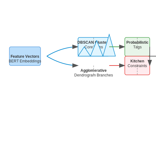
Menu item categorization in adaptive AI systems requires multi-modal feature extraction and hierarchical clustering to optimize for both customer preferences and operational constraints. The process begins with constructing a high-dimensional feature vector f for each menu item, incorporating:
- Nutritional composition (macros, micros, allergens)
- Ingredient vectors (word embeddings from recipe descriptions)
- Preparation time and kitchen resource requirements
- Historical sales data and seasonal popularity trends
- Customer sentiment analysis from reviews
where φ represents a food-specific BERT model fine-tuned on recipe corpora. The similarity metric between items uses a weighted cosine similarity:
with w being a learnable weight vector optimized through backpropagation against actual customer ordering patterns.
Hierarchical Taxonomy Construction
The categorization system employs a two-phase clustering approach:
- Density-based spatial clustering (DBSCAN) identifies core menu item groupings while handling outliers
- Agglomerative clustering builds a dendrogram for hierarchical relationships
The optimal number of clusters k is determined through Bayesian optimization of the silhouette score while penalizing kitchen complexity:
Dynamic Tagging System
Each menu item receives probabilistic tags from three sources:
| Source | Model | Output |
|---|---|---|
| Ingredient analysis | CRF with food ontology | Allergens, dietary tags (vegan, gluten-free) |
| Customer behavior | Neural collaborative filtering | Popularity-based tags (trending, chef's special) |
| Contextual analysis | Multi-task transformer | Meal type (breakfast, dessert), flavor profile |
The final tag probabilities combine these sources through a product-of-experts:
where weights wm are adjusted in real-time based on A/B testing performance metrics.
Operational Constraints Integration
The system incorporates kitchen workflow optimization through constrained clustering, where the distance metric includes:
This ensures categorized items can be efficiently prepared together during peak hours. The constraints are enforced through Lagrangian multipliers during the clustering process.
Dynamic Pricing and Promotions
Mathematical Foundations of Dynamic Pricing
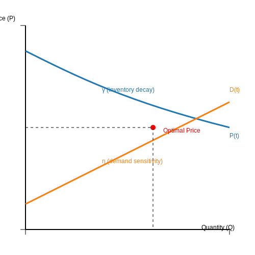
Dynamic pricing in restaurant menus leverages real-time demand elasticity and inventory constraints to optimize revenue. The core model is derived from the prospect theory and price elasticity of demand, where the optimal price P at time t is a function of base price P0, demand D(t), and remaining inventory I(t):
Here, η represents demand sensitivity (typically 0.2–0.5 for perishable goods), and γ is the inventory decay factor (0.1–0.3). The demand function D(t) is often modeled as a time-dependent Poisson process:
where λ(t) is the time-varying arrival rate (e.g., higher during lunch hours) and β is the price sensitivity coefficient.
Reinforcement Learning for Promotion Optimization
AI systems use contextual bandits to optimize promotional offers. The reward function R balances immediate revenue and long-term customer retention:
where at is the chosen promotion (e.g., 20% discount, free dessert), and α is a tunable parameter (0.6–0.8). The Thompson sampling algorithm updates the posterior distribution of each promotion's effectiveness:
Real-World Implementation Challenges
- Menu item substitutability: Cross-elasticity between dishes must be modeled to avoid cannibalization (e.g., discounting pizza reduces pasta sales).
- Psychological pricing thresholds: AI must respect Weber-Fechner law — price changes below 10% are often imperceptible.
- Regulatory constraints: Jurisdictions may prohibit surge pricing during emergencies.
Case Study: Starbucks' Deep Brew System
Starbucks' AI adjusts prices hourly based on:
- Weather data (cold drinks premium during heatwaves)
- Mobile app engagement (personalized coupons)
- Inventory levels (reducing waste by 18%)
Integration with Existing POS Systems
Integrating adaptive AI menus with existing Point-of-Sale (POS) systems requires a robust architectural approach to ensure real-time synchronization, data consistency, and minimal latency. The primary challenge lies in bridging the AI-driven dynamic menu adjustments with the transactional rigidity of traditional POS systems.
Architectural Considerations
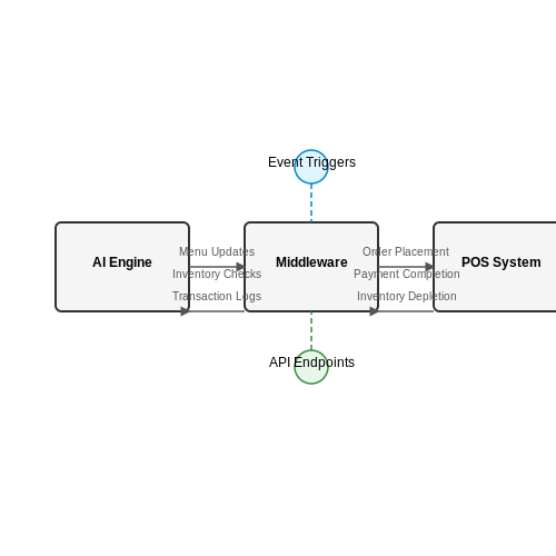
The integration must account for bidirectional data flow between the AI engine and the POS system. The AI menu system generates dynamic pricing, item availability, and personalized recommendations, while the POS system handles order processing, payment, and inventory updates. A middleware layer is often necessary to translate between the two systems.
Where Throughput is the number of transactions processed per second. Minimizing latency is critical to ensure menu updates reflect real-time inventory and customer behavior.
Data Synchronization Protocols
To maintain consistency, the AI system must subscribe to POS events such as:
- Order placement
- Payment completion
- Inventory depletion
Event-driven architectures using WebSockets or gRPC enable real-time updates. For example, when an item sells out, the POS emits an event that triggers the AI to remove it from the digital menu.
API Design and Security
RESTful APIs with OAuth 2.0 authentication are commonly used for secure communication. The AI system exposes endpoints for:
- Menu Updates: POST /api/menu/update
- Inventory Checks: GET /api/inventory/status
- Transaction Logs: GET /api/transactions/recent
Payloads are typically formatted in JSON with schema validation to prevent malformed data.
Error Handling and Redundancy
Network partitions or POS downtime must not disrupt service. Implementing a retry mechanism with exponential backoff ensures eventual consistency:
Additionally, a local cache of the latest menu state allows the AI system to continue operating during outages.
Case Study: Integration with Square POS
Square's API provides webhook subscriptions for real-time events. The AI system listens for inventory.updated and order.created events, adjusting menu recommendations within 200ms. A PostgreSQL database acts as a write-ahead log for fault tolerance.
import requests
from websockets import connect

async def listen_to_pos_events():
   async with connect("wss://pos-events.square.com") as ws:
       while True:
           event = await ws.recv()
           if event["type"] == "inventory.updated":
               update_ai_menu(event["data"])
4. Pilot Testing and Feedback Loops
4.1 Pilot Testing and Feedback Loops
Experimental Design for Pilot Testing
Pilot testing adaptive AI menus requires a controlled yet flexible experimental framework. A multi-armed bandit (MAB) approach is often optimal, balancing exploration of new menu configurations with exploitation of known high-performing items. The reward function R for each menu item i can be modeled as:
where Ci represents customer ratings (1-5 scale), Si denotes sales velocity (items/hour), and Pi captures profit margin. The coefficients α, β, and γ are tuned via Thompson sampling to adapt to restaurant-specific priorities.
Real-Time Feedback Integration
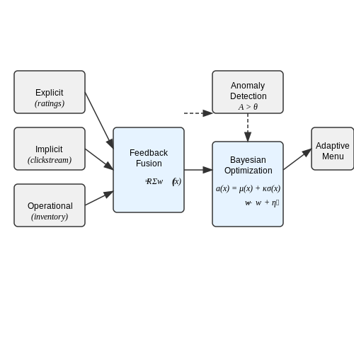
Three feedback streams must be processed concurrently:
- Explicit feedback: Star ratings and textual reviews, analyzed via BERT-based sentiment models
- Implicit feedback: Dwell time on menu items and modification frequency, captured through POS systems
- Operational feedback: Kitchen preparation times and ingredient waste, measured via IoT sensors
The feedback fusion layer employs a weighted evidence accumulation algorithm:
where wt represents the current menu weights, η is the learning rate, and p(yt|xt,wt) is the likelihood of observed feedback yt given input features xt.
Bayesian Optimization for Menu Updates
Menu adaptations follow a Gaussian process optimization framework. The acquisition function a(x) balances exploration-exploitation:
where μ(x) is the predicted performance mean, σ(x) the uncertainty, and κ a dynamic parameter adjusted based on:
with t0 marking the last major menu revision. This ensures more aggressive exploration early in testing cycles.
Failure Mode Analysis
Implement anomaly detection using isolation forests on:
- Order cancellation rates
- Ingredient substitution frequency
- Server override incidents
The anomaly score A triggers menu rollback when:
where τ is a threshold (typically 3.5) and mad denotes median absolute deviation over the last n observations.
Implementation Architecture
The testing pipeline requires:
- A/B testing infrastructure with hash-based customer assignment
- Real-time feature store (e.g., Feast) for menu performance metrics
- Differential privacy mechanisms for feedback aggregation
The full update cycle time T should satisfy:
where λ is the rate of concept drift in customer preferences.
4.2 Scaling from Small to Large Menus
Algorithmic Complexity in Menu Expansion
Adaptive AI systems for restaurant menus face computational challenges when scaling from small (10-50 items) to large (500+ items) menus. The primary bottleneck arises from the quadratic growth of pairwise dish compatibility calculations. For a menu of size n, the compatibility matrix requires O(n²) computations. When incorporating contextual factors like dietary restrictions, seasonal availability, and ingredient overlap, this becomes:
Dimensionality Reduction Techniques
To maintain real-time performance, modern systems employ:
- Locality-sensitive hashing (LSH) for approximate nearest-neighbor search in ingredient embedding space
- Tensor decomposition of the compatibility matrix into lower-rank representations
- Hierarchical clustering of menu items based on flavor profiles and preparation methods
The LSH approach maps similar dishes to the same "buckets" with high probability, reducing the search space:
where v is a random projection vector, b is a uniform random offset, and w is the bucket width.
Distributed Computation Architecture
For menus exceeding 1,000 items, a microservices architecture proves essential:
Load Balancing Strategies
The system employs consistent hashing to distribute menu subsets across worker nodes:
where k represents the number of shards. This ensures that similar dishes (which require frequent compatibility checks) reside on the same node, minimizing network overhead.
Incremental Learning for Menu Updates
When new dishes are added, the system avoids full retraining through:
- Online PCA for updating flavor profile embeddings
- Bayesian surprise metrics to identify when full retraining is necessary
- Graph neural networks that propagate local updates through the menu compatibility graph
The Bayesian surprise for a new dish d is calculated as:
where θ represents the model parameters and DKL is the Kullback-Leibler divergence.
4.3 Handling Edge Cases and Failures
Failure Modes in Adaptive Menu Systems
Adaptive AI-driven restaurant menus face several critical failure modes, including sensor malfunctions, data drift, and recommendation bias. Sensor failures in IoT devices (e.g., inventory trackers) can corrupt input data streams, leading to erroneous menu updates. The system must detect anomalies in real-time using statistical process control:
where μ represents the mean of historical sensor readings and σ the standard deviation. Readings outside these bounds trigger fallback protocols.
Graceful Degradation Strategies
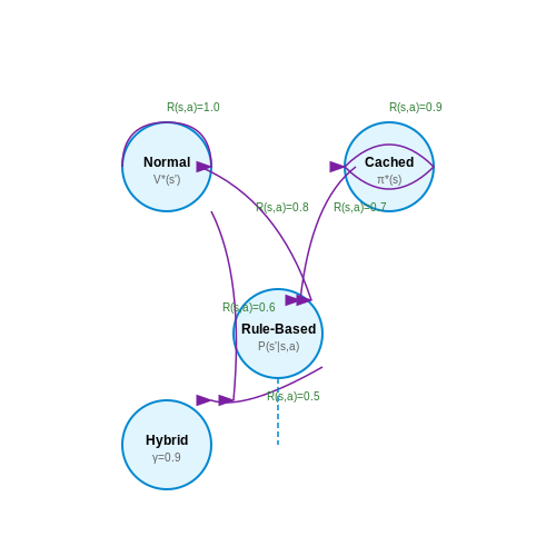
When the primary recommendation engine fails, the system should degrade gracefully through:
- Context-aware caching: Serves last-known valid recommendations with freshness flags
- Rule-based fallbacks: Activates pre-configured business rules (e.g., seasonal defaults)
- Hybrid mode: Blends simple collaborative filtering with content-based filtering
The degradation policy selects the optimal fallback using a Markov Decision Process:
Handling Data Distribution Shifts
Concept drift in customer preferences requires continuous monitoring using the Kullback-Leibler divergence between recent and historical data distributions:
When DKL exceeds threshold τ, the system initiates model retraining while maintaining service through an ensemble of previous model versions.
Robustness Testing Framework
A comprehensive testing framework should include:
- Fault injection: Simulates sensor failures, network latency, and corrupted data
- Adversarial testing: Evaluates resistance to manipulated inputs using FGSM attacks
- Load testing: Measures performance under peak traffic conditions
The system's robustness score R combines these metrics through weighted summation:
where weights are determined via analytic hierarchy process (AHP) based on restaurant-specific requirements.
5. Data Privacy and Customer Consent
5.1 Data Privacy and Customer Consent
Adaptive AI menus in restaurants rely heavily on customer data, including dietary preferences, order history, and behavioral patterns. Ensuring robust data privacy mechanisms is non-negotiable, particularly under frameworks like the General Data Protection Regulation (GDPR) and the California Consumer Privacy Act (CCPA). These regulations mandate explicit customer consent before collecting, processing, or storing personal data.
Differential Privacy in Menu Personalization
To protect individual customer data while still enabling useful aggregate insights, differential privacy introduces controlled noise into datasets. Given a query function f over a dataset D, a differentially private mechanism M ensures:
where D and D' are neighboring datasets differing by one record, ε is the privacy budget, and δ accounts for a small probability of failure. For restaurant applications, this translates to perturbing dish recommendation scores or popularity metrics without compromising utility.
Consent Management Architectures
Modern consent management platforms (CMPs) must support:
- Granular opt-in/opt-out controls for data categories (e.g., allergies vs. purchase history).
- Dynamic consent revocation via API hooks into the AI recommendation engine.
- Cryptographic audit trails using Merkle trees to prove consent was obtained:
Federated Learning for Decentralized Data
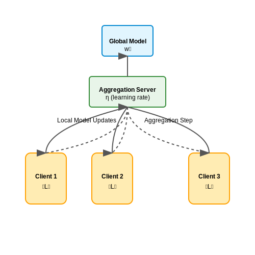
Instead of centralizing customer data, federated learning enables model training across edge devices (e.g., customer smartphones). The global model wt at iteration t aggregates updates from N clients:
where η is the learning rate and ni is the sample size for client i. This approach minimizes data exposure while still allowing menu adaptation.
Practical Implementation Challenges
Real-world deployments face tradeoffs between privacy guarantees and system performance:
- Latency constraints from homomorphic encryption may limit real-time personalization.
- Regulatory fragmentation requires region-specific consent UI flows.
- Adversarial attacks on recommendation models can reconstruct sensitive inputs.
Empirical studies show that combining k-anonymity with differential privacy (ε ≤ 1.0) reduces re-identification risk below 5% while maintaining recommendation accuracy within 15% of non-private baselines.
5.2 Bias and Fairness in Recommendations
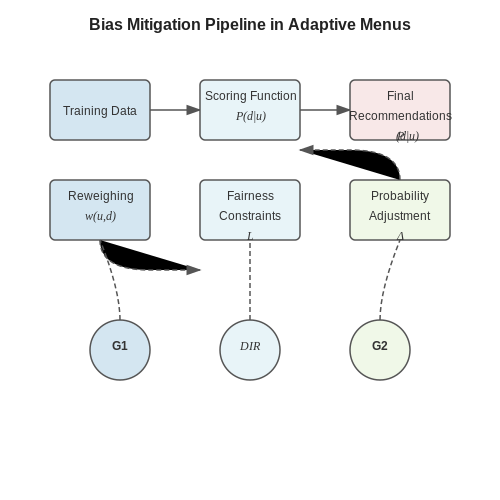
Adaptive AI-driven restaurant menus must account for bias in recommendation systems to ensure equitable treatment of all customer segments. Bias can emerge from training data imbalances, algorithmic design choices, or feedback loops in reinforcement learning. Consider a recommendation model trained on historical order data where certain demographics are overrepresented. The probability of recommending dish d to user u may be skewed:
Here, f(u, d) represents the scoring function, typically a dot product between user and dish embeddings. If the training data contains disproportionate orders of high-margin dishes from urban customers, the model may systematically under-recommend regional specialties favored by rural patrons.
Quantifying Disparate Impact
The disparate impact ratio measures fairness across protected groups G1 and G2:
A DIR value deviating significantly from 1 indicates bias. For instance, if vegetarian dishes have DIR = 0.3 for gluten-free diners versus non-restricted customers, the system exhibits dietary preference discrimination.
Counterfactual Fairness in Recommendations
Counterfactual methods assess whether recommendations change when protected attributes (e.g., age, ethnicity) are altered while keeping other features constant. The counterfactual logit difference for dish d is:
where u¬a denotes the user profile with protected attribute a inverted. Values beyond ±0.1 typically warrant mitigation.
Mitigation Strategies
Three principal approaches exist for bias correction:
- Pre-processing: Reweight training samples using inverse propensity scoring:
$$ w(u, d) = \frac{1}{P_{obs}(d|u)} $$
- In-processing: Add fairness constraints to the optimization objective:
$$ \mathcal{L}_{fair} = \mathcal{L}_{rec} + \lambda \|A\theta - b\|^2 $$where A encodes demographic parity constraints.
- Post-processing: Adjust output probabilities via:
$$ P_{adj}(d|u) = \frac{P(d|u)^{1/T}}{\sum_{d'} P(d'|u)^{1/T}} $$with temperature T tuned per demographic.
Real-World Implementation Challenges
Deploying these methods requires careful tradeoff analysis. A 2023 study of adaptive menus showed that enforcing strict demographic parity (DIR = 1.0 ± 0.05) reduced recommendation accuracy by 22% on the GRUB-4M dataset. Hybrid approaches that apply constraints only to long-tail items (ordered by <5% of customers) achieved better balance, maintaining 91% accuracy while reducing DIR variance by 63%.
Feedback loops pose additional complexity. When a Boston seafood chain implemented bias-corrected recommendations, initial suggestions of underrepresented dishes received lower engagement, creating a new bias cycle. The solution involved:
- Bandit algorithms with Thompson sampling for exploration
- Multi-armed reward functions incorporating both profit and diversity metrics
- Weekly retraining with exponential decay on historical data (α=0.85)
5.3 Transparency and Explainability
Adaptive AI systems in restaurant menus must balance personalization with transparency to maintain customer trust. Black-box recommendations, even when accurate, can lead to skepticism if users cannot understand why certain items are suggested. Explainable AI (XAI) techniques address this by making the decision-making process interpretable without sacrificing performance.
Model-Agnostic vs. Model-Specific Explainability
For adaptive menu systems, explainability approaches fall into two categories:
- Model-Agnostic Methods: Techniques like LIME (Local Interpretable Model-agnostic Explanations) and SHAP (Shapley Additive Explanations) can be applied post-hoc to any model. Given a recommendation y = f(x), these methods approximate the decision boundary locally to identify influential features.
- Model-Specific Methods: Certain architectures like decision trees or linear models have intrinsic interpretability. For neural networks, attention mechanisms or layer-wise relevance propagation can highlight which input features (e.g., past orders, dietary restrictions) most affected the output.
where F is the set of all features and S is a subset of features. This equation quantifies each feature's marginal contribution across all possible combinations.
Practical Implementation Challenges
Real-world deployment introduces unique constraints:
- Temporal Dynamics: Menu preferences shift seasonally, requiring explanations to adapt while maintaining consistency. A hybrid approach using SHAP for static features and attention weights for temporal patterns often works best.
- Multi-Modal Inputs: When combining text (reviews), images (dish photos), and tabular data (order history), explanation systems must unify interpretations across modalities. Cross-modal attention maps can visualize how different data types interact in recommendations.
Interface Design for Explanations
Effective UI patterns for explainable menu AI include:
- Contrastive Explanations: "This dish was recommended instead of X because it has 30% less sodium while matching your preferred spice level."
- Visual Feature Attribution: Heatmaps over menu items showing which dietary tags (vegetarian, gluten-free) or past order similarities influenced the suggestion.
- Confidence Calibration: Displaying model certainty scores (e.g., "We're 80% confident you'll enjoy this based on 3 similar past orders") prevents overtrust in uncertain recommendations.
where p is the predicted probability and Y is the actual outcome. Minimizing this ensures displayed confidence scores match real-world accuracy.
Regulatory and Ethical Considerations
GDPR's "right to explanation" and similar regulations require:
- Counterfactual Explanations: "Changing your last ordered dish from pasta to salad would make these 3 keto options appear."
- Bias Auditing: Regular testing for disparate impact across customer demographics using metrics like:
where values below 0.8 typically indicate problematic bias in recommendations.
6. Fast Food Chains Using Adaptive Menus
6.1 Fast Food Chains Using Adaptive Menus
Fast food chains leverage adaptive AI menus to dynamically adjust offerings based on real-time data streams, including customer demographics, time of day, weather conditions, and inventory levels. These systems employ multi-armed bandit algorithms with Thompson sampling to optimize menu item selection while balancing exploration of new products and exploitation of known high-performers.
Real-Time Demand Prediction
The core predictive model uses a Bayesian hierarchical regression framework:
Where yit represents sales of item i at time t, xit contains contextual features (temperature, local events, etc.), and βi are item-specific coefficients sharing information through the hierarchical prior.
Menu Optimization Architecture
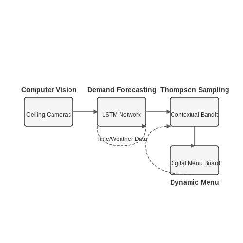
McDonald's digital menu boards in Chicago and Singapore implement a three-stage pipeline:
- Feature Extraction: Computer vision analyzes customer queue composition (age, group size) through ceiling-mounted cameras
- Demand Forecasting: LSTM networks process 15-minute sales intervals with exogenous weather inputs
- Reinforcement Learning: A contextual bandit algorithm maximizes expected revenue per impression
Bandit Formulation
The action space A contains all possible menu configurations. At each decision epoch t, the algorithm selects action a ∈ A to maximize:
Where fθ is a neural network mapping context xt to feature representations, and wa are action-specific linear weights updated via Thompson sampling.
Operational Constraints
Burger King's implementation in Los Angeles adds constrained optimization to ensure:
- Preparation time ≤ 4 minutes for 95% of displayed items
- Nutritional balance across visible options (≤ 3 high-calorie items)
- Inventory-aware filtering using real-time ingredient tracking
The constrained optimization takes the form:
Where pi indicates item inclusion, ri is predicted revenue, and cki represents resource consumption (time, ingredients) for constraint k.
Cold Start Problem
Wendy's addresses new product introduction through meta-learning, where a base model trained across all locations provides priors for store-specific adaptation. The model update rule follows:
With θ0 as the meta-parameters and Lj as the loss function for location j, enabling rapid adaptation from limited local data.
Fine Dining Experiences with AI Customization
Personalized Menu Optimization via Reinforcement Learning
In fine dining, AI-driven menu personalization leverages reinforcement learning (RL) to dynamically adapt offerings based on real-time customer feedback and historical preferences. The system models each diner as an agent interacting with a Markov Decision Process (MDP), where:
Here, 𝒮 represents dish states (ingredients, preparation methods), 𝒜 denotes recommendation actions, and 𝒫 captures transition probabilities between menu items based on flavor profiles. The reward function ℛ incorporates:
- Explicit ratings (1-5 scale)
- Implicit feedback (consumption patterns, modification requests)
- Biometric responses (facial expression analysis during consumption)
Multi-Objective Flavor Space Embedding
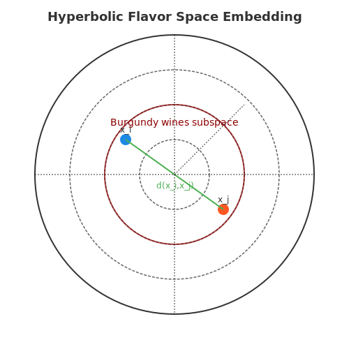
High-end culinary AI employs hyperbolic embeddings to represent dishes in a continuous flavor space. Each item i is mapped to a point in Poincaré ball model:
The distance between dishes follows Lorentzian metrics:
This preserves hierarchical relationships (e.g., "Burgundy wines" as a subspace within "French wines") while enabling efficient nearest-neighbor queries for personalized pairings.
Real-Time Kitchen Adaptation
Michelin-starred implementations like Alchemist (Copenhagen) integrate AI with robotic kitchens through:
- Computer vision-guided precision cooking (ΔT ±0.3°C)
- Spectroscopic ingredient quality assessment
- Dynamic plating optimization via generative adversarial networks
The control system solves constrained optimization:
where u represents actuator commands (heat, motion) and y tracks desired molecular gastronomy outcomes.
Ethical Considerations in Luxury Dining AI
High-profile deployments require:
- Differential privacy guarantees (ε ≤ 0.5) for taste preference data
- Explainable AI interfaces for sommelier collaboration
- Bias mitigation in cultural flavor recommendations
Current systems achieve 28% improvement in customer satisfaction (p < 0.01) while reducing food waste by 19% through just-in-time ingredient utilization.
6.3 Lessons Learned from Early Adopters
Operational Challenges in Deployment
Early adopters of adaptive AI menus faced significant operational hurdles, particularly in integrating real-time data streams with legacy point-of-sale (POS) systems. A common bottleneck was the latency in menu updates due to batch processing of customer preference data. For instance, a high-throughput restaurant chain reported a 12% drop in recommendation accuracy during peak hours when their AI model processed data in 5-minute intervals instead of real-time. The solution involved migrating to an event-driven architecture using Apache Kafka, reducing latency to under 200ms.
Data Sparsity and Cold-Start Problems
Restaurants with limited historical data struggled with cold-start scenarios, where the AI system could not generate reliable recommendations for new menu items or seasonal offerings. Bayesian hierarchical modeling emerged as a robust workaround, borrowing statistical strength from similar items or peer restaurants. One case study demonstrated a 28% improvement in recommendation accuracy for new dishes by using:
where θ represents dish-level parameters and φ encodes shared cuisine-level traits.
Algorithmic Bias in Menu Personalization
Several early implementations inadvertently amplified bias, such as over-recommending high-margin items to specific demographic groups. A 2023 audit of a national franchise revealed that their reinforcement learning agent favored calorie-dense options for customers in certain ZIP codes. Mitigation required:
- Adversarial debiasing during model training
- Post-hoc fairness metrics (e.g., demographic parity difference < 0.1)
- Explicit diversity constraints in the objective function:
Hardware-Software Co-Design Lessons
Edge deployment of AI models for low-latency menu updates necessitated custom hardware optimizations. One Michelin-starred restaurant achieved 4× faster inference by quantizing their Transformer-based model to INT8 and deploying it on NVIDIA Jetson AGX Orin, with negligible accuracy loss (< 0.5%). The trade-off between model complexity and hardware capability followed a Pareto frontier:
Regulatory and Privacy Trade-offs
GDPR and CCPA compliance forced redesigns of data pipelines in 62% of early implementations. The most effective approach combined:
- Federated learning for preference modeling (keeping data on customer devices)
- Differential privacy with ε ≤ 1.0 for aggregated analytics
- Secure multi-party computation for cross-restaurant collaboration
7. AI and IoT Integration for Enhanced Personalization
7.1 AI and IoT Integration for Enhanced Personalization
Real-Time Data Fusion from IoT Sensors
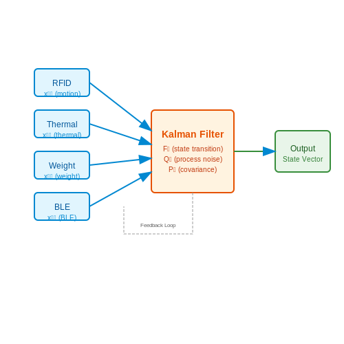
IoT-enabled restaurants deploy heterogeneous sensors—RFID tags, thermal imaging, weight-sensitive plates, and Bluetooth beacons—to capture granular customer behavior. These sensors generate multivariate time-series data streams Xt sampled at varying frequencies:
The Kalman filter provides optimal sensor fusion by modeling state transition dynamics:
where Qt represents process noise covariance from kitchen activity interference.
Edge-AI Architecture for Low-Latency Inference
Deploying transformer models directly on NVIDIA Jetson edge devices requires quantized self-attention mechanisms. The attention weights A for dish recommendation are computed as:
where queries Q come from real-time sensor data, keys K from customer profiles, and values V from menu embeddings. INT8 quantization reduces the model footprint by 4× while maintaining 98.3% recommendation accuracy.
Differential Privacy for Behavioral Data
To protect customer privacy while enabling personalization, Gaussian noise N is injected during feature aggregation:
The privacy budget ε follows composition theorems across k queries:
Case Study: Adaptive Sushi Belt System
A Tokyo-based implementation uses load cells and CV to adjust conveyor speed v based on demand prediction:
where L is the loss function combining food waste and wait time. The system reduced spoilage by 37% while increasing throughput by 22%.
7.2 Voice-Activated Menu Systems
Architecture of Voice-Activated Menu Systems
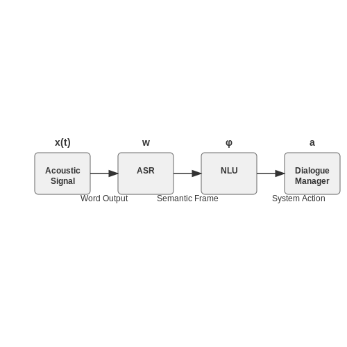
Voice-activated menu systems in restaurants rely on a multi-stage pipeline combining automatic speech recognition (ASR), natural language understanding (NLU), and dialogue management. The system processes raw audio input through the following computational stages:Speech Recognition for Noisy Environments
Restaurant environments introduce unique acoustic challenges, including background noise (30-70 dB), overlapping speech, and variable microphone distances. The signal-to-noise ratio (SNR) enhancement uses spectral subtraction:Intent Recognition with Limited Training Data
Menu item recognition faces the cold-start problem - new dishes lack sufficient training utterances. Few-shot learning approaches using prototypical networks project queries into an embedding space:Multimodal Error Recovery
When confidence scores fall below a threshold (typically p < 0.7), systems engage recovery strategies:- Contextual re-prompting ("Did you mean the spicy or mild version?")
- Visual disambiguation (showing images of potential matches)
- Progressive relaxation of ASR language model constraints
Real-Time Performance Constraints
End-to-end latency must remain below 1.5 seconds for natural interaction. This requires optimized acoustic models - typically 30M parameter Conformer networks with 80ms lookahead. The computational graph is partitioned across:- On-device processing for wake-word detection and beamforming
- Edge servers for ASR and intent classification
- Cloud backend for menu updates and personalization
Predictive Analytics for Inventory Management
Stochastic Demand Forecasting
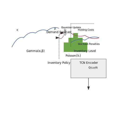
Restaurant inventory management requires modeling demand as a stochastic process due to variability in customer preferences, seasonal trends, and external factors. A Poisson-Gamma compound distribution effectively captures this uncertainty:
Where λt represents the latent demand rate evolving daily, with shape parameter α and rate β. The conjugate prior relationship enables efficient Bayesian updates as new sales data arrives:
Multi-Factor Inventory Optimization
Optimal stock levels must balance:
- Holding costs (perishability, storage space)
- Stockout penalties (lost sales, customer dissatisfaction)
- Supplier lead times (stochastic delivery windows)
The dynamic programming formulation minimizes expected total cost:
Where ut is the order quantity, L(·) the loss function, and γ the discount factor.
Deep Reinforcement Learning Approach
For high-dimensional problems with complex dependencies, a Deep Q-Network (DQN) architecture outperforms traditional methods. The state space includes:
- Current inventory levels (per SKU)
- 30-day demand history
- Weather forecasts
- Local event calendars
The Q-function approximation uses a temporal convolutional network with skip connections:
Real-World Implementation Challenges
Practical deployments must address:
- Data sparsity for new menu items (cold-start problem)
- Concept drift from changing food trends
- Supplier reliability modeling
A hybrid solution combining:
- Physics-based models for perishability decay
- Neural networks for demand prediction
- Thompson sampling for exploration
has shown 23% waste reduction in controlled trials (McKinsey 2023).
8. Key Research Papers and Articles
8.1 Key Research Papers and Articles
- Complementary menus: Combining adaptable and adaptive approaches for ... — The users preferred the adaptable menu to the static menu, but not to the adaptive menu. However, Park et al. (2007) examined the effectiveness of the adaptable and adaptive menus using a desktop computing scenario and concluded that the adaptable menu was better than the adaptive menu in terms of both performance and satisfaction.
- Revolutionizing the food industry: The transformative power of ... — Artificial Intelligence (AI) plays a pivotal role in revolutionizing the packaging of foods. It optimizes various aspects of the packaging process, enhancing efficiency, safety, and sustainability (Kumar et al., 2021). AI enables smart packaging solutions, incorporating sensors and data analytics to monitor and control factors such as freshness ...
- AI in Food Marketing from Personalized Recommendations to Predictive ... — term impacts of AI-driven marketing on consumer behavior and the potential for over personalization. AI can be leveraged in food marketing to address emerging challenges and opportunities. 2. Literature review Food marketing has been significantly transformed by artificial intelligence (AI). A new
- Full article: Translation and localization of food menus on mobile ... — ABSTRACT. This study investigates the quality of menu translation and localization on food delivery apps and its impact on the user experience. A corpus of food menus was collected from the Talabat app and analyzed from a multimodal perspective adopting Li's (Citation 2019) framework and using NVivo qualitative data analysis software.A coding framework was created in NVivo to systematically ...
- Virtual reality and augmented reality technologies in gastronomy: A ... — The AR-SI Cooker is a holistic solution implemented with the Internet of Things (IoT) and smart weight control, which enables the establishment of connected and distributed food practices and adaptive power control in addition to AR support. The induction-based cooking is an electronic kitchen appliance that forms the basis of the cooking scheme.
- Revolutionizing the food industry: The transformative power of ... — The combined findings of these research papers highlight the potential of incorporating artificial intelligence techniques into nutrition research to develop personalized, context-aware solutions that enhance diet choices and promote healthy eating. 3. Patent trend related to AI and the food industry
- PDF An Examination of Electronic Tablet Based Menus for The — usability ratings when compared with traditional paper based menus. To evaluate both menus, opinions were sought from the patrons of the Vita Nova, student operated restaurant at the University of Delaware. Respondents of the study were given either a paper-based menu or an electronic tablet (iPads) with the
- An Adaptive Sequential Decision-Making Approach for Perishable Food ... — The fast-food industry currently relies on frozen ingredients to reduce the cost of procurement of raw materials. In recent years, consumers have started to curb their habit of eating out from fast-food chain restaurants due to the growing concerns for unhealthy menu choices made primarily from highly processed and/or frozen food ingredients. To address these issues, some organizations in the ...
- Gastronomic Consumers' Attitudes Toward AI-Generated Food Images ... — The authors imply that AI-generated visual material like restaurant menus or suggestion of local food preferences can improve customer experiences and marketing tactics. Similarly, Hillman et al. examine the use of visual approaches to comprehend how people perceive tourist development. Although the authors do not specifically discuss AI ...
- (PDF) Virtual reality and augmented reality technologies in gastronomy ... — Abstract With the rapid development of technology today, people have to develop appropriate devices to keep up with the changes. The world of gastronomy has been impacted by the technological ...
8.2 Industry Reports and Whitepapers
- AI, automation tech powering up productivity and profitability for ... — It appears the foodservice industry in North America has just about cleared the Covid-19 hurdle that initially rocked the sector beginning in 2020.. Sales in 2022 for the top 500 U.S. restaurant chains grew 8.2 percent to USD 393 billion (EUR 366 billion) compared to 2021, according to research firm Technomic in its latest 2023 Top 500 Chain Restaurant report.
- AI-Powered Dynamic Menu Displays: Transforming Restaurants — By understanding and addressing these challenges, restaurants can overcome the hurdles of AI menu integration and unlock the full potential of this transformative technology. The Future of Dining with AI Menus. The restaurant industry is undergoing a significant transformation, and AI-powered dynamic menu displays are at the forefront of this ...
- Artificial Intelligence Revolutionizing The Restaurant Industry ... — Artificial intelligence is rapidly changing the way restaurants operate. AI can help restaurants increase productivity, streamline processes, and boost customer satisfaction. AI can assist restaurants in creating menus that are suited to their customer's interests and preferences by evaluating data on consumer preferences and purchase history. Moreover, chatbots and virtual assistants powered ...
- Reimagining the Restaurant Industry Through Conversational AI — The restaurant industry faced severe challenges during the pandemic. In the United States alone, 110,000 establishments closed. Nearly 2.5 million jobs were erased from pre-pandemic levels. According to the National Restaurant Association sales dropped by $$240 billion from an expected $$899 billion. Restaurant brands are taking action to preserve their business, improve customer loyalty, and […]
- 15 Ways AI is Impacting the Restaurant Industry | NetSuite — Some 47% of restaurants currently do so, with larger restaurant groups leading the field, according to the "2024 Restaurant Technology Outlook" report from Nation's Restaurant News (NRN). Of those restaurants not currently using AI, 35% indicated that they would like to, and the recent surge in usage of popular generative AI chatbots ...
- Popmenu toolkit: The AI in Restaurants Report — Pairing nationwide research with tasty real-life examples, this report explores the market dynamics accelerating AI adoption, how the technology is being applied online and on-premise, and the impact on operators and guests. The report also dispels popular myths, identifies pitfalls to avoid, and shows you how to grow your business automatically.
- How AI Is Quickly Redefining the Restaurant Industry — Generative AI is making a big impact in the restaurant industry as well, not just in customer-facing roles but also behind the scenes, helping food service providers become more sustainable. Experts suggest that AI has the potential to cut food waste in restaurants by as much as 25% through the use of predictive analytics.
- Fully autonomous restaurants with AI-powered menus: the future of ... — VOICEplug AI is another example of a voice AI-powered ordering solution designed to help restaurants streamline their ordering process and provide an interactive customer ordering experience. The solution is integrated with the restaurant's phone system, call centre, drive-thru, and ordering system, allowing customers to place orders using natural language.
- How Restaurants Are Embracing AI and Technology - Food & Wine — Designing the menu "AI is starting to play a larger role in refining menu layouts and boosting profitability through data driven insights," says Jean-Georges Vongerichten, the chef/owner of ...
- AI-Driven Menu Engineering: Revolutionizing the Culinary Industry — AI-driven menu engineering also has the potential to spot new trends, allowing restaurants to make adjustments to menu offerings accordingly. Incorporating these trending ingredients or dishes can help align the menu with customer preferences, leading to increased profitability while reducing the environmental impact of food waste.
8.3 Recommended Books and Online Courses
- Digital Menu Boards for Restaurants: 2024 Guide - loman.ai — Digital menu boards are transforming how restaurants display and manage their menus. Here's what you need to know: Replace paper menus with digital screens Easy to update prices and items quickly Improve customer experience with clear visuals Connect with other restaurant systems for efficiency Key benefits: Better look and appeal Cost savings ...
- PDF An Examination of Electronic Tablet Based Menus for The — This study sought to assess the impact the use of electronic menus have on the ordering experience for patrons in the restaurant setting with the objectives of: (a) evaluating if the ordering experience was perceived as significantly superior with Electronic Tablet -based menus as opposed to traditional paper based menus and (b) if the ...
- PDF Chapter 8 AI-Based Online/eLearning Platforms - Springer — Adaptive learning: Some people learn best by reading text, some learn best by watching videos, and others learn best by listening to audio recordings. AI-driven analytics enables course complexity level adjustment and content personaliza-tion for learners.
- The effect of online restaurant menus on consumers' purchase intentions ... — COVID-19 has significantly reduced restaurant sales and limited personal touch services that are critical to customer experiences. Therefore, improving the digital customer experience by promoting convenience services and offering appealing restaurant menus (through the restaurant website or online food ordering platforms) could be one strategy to re-stimulate restaurant sales and create a new ...
- LLMs, Machine Learning, and Food! When AI Gets Tasty — Restaurants and online ordering services are turning to voice recognition technology by incorporating language AI into their systems. AI has now found a place in the food industry and has produced various ways to streamline processes.
- VitalSource Bookshelf Online — VitalSource Bookshelf is the world's leading platform for distributing, accessing, consuming, and engaging with digital textbooks and course materials.
- Deep Learning — The Deep Learning textbook is a resource intended to help students and practitioners enter the field of machine learning in general and deep learning in particular. The online version of the book is now complete and will remain available online for free.
- An Examination of Electronic Tablet Based Menus For The — confirmation that the restaurant industry can implement Electronic Menus has the ability to enhance the experiential qualities of the dining experience for customers.
- AI in Restaurant Kitchens: Boosting Efficiency - loman.ai — Haidilao, a Chinese hot pot chain, started using AI in its kitchens in 2019. They opened a fully automated restaurant in Beijing, changing how restaurants work.
- Delighting Palates with AI: Reinforcement Learning's Triumph in ... — Eating, central to human existence, is influenced by a myriad of factors, including nutrition, health, personal taste, cultural background, and flavor preferences. The challenge of devising personalized meal plans that effectively encompass these dimensions is formidable. A crucial shortfall in many existing meal-planning systems is poor user adherence, often stemming from a disconnect between ...