Training Swarm-based RL Agents
1. Key Concepts in Swarm Intelligence
Key Concepts in Swarm Intelligence
Emergent Behavior and Self-Organization
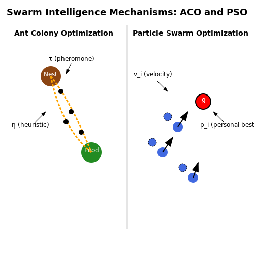
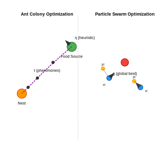
Swarm intelligence (SI) systems exhibit emergent behavior, where complex global patterns arise from simple local interactions among agents. This phenomenon is rooted in self-organization, a process where decentralized components collectively adapt to environmental changes without centralized control. For example, ant colonies optimize foraging paths through pheromone trails—a stigmergic communication mechanism where agents modify their environment to influence others' behavior.
Here, pij is the probability of an ant moving from node i to j, τij represents pheromone intensity, and ηij is the heuristic desirability (e.g., inverse distance). The exponents α and β weight the influence of pheromones versus heuristic information.
Decentralized Control and Scalability
SI systems rely on decentralized decision-making, where agents operate autonomously using local information. This contrasts with centralized systems that require global state awareness. Decentralization enables scalability: adding more agents typically improves performance without redesigning the system. Particle swarm optimization (PSO) exemplifies this, where particles update velocities based on personal and neighborhood best solutions:
vi is the particle velocity, w is inertia, c1, c2 are learning coefficients, and r1, r2 are random numbers in [0,1]. The terms pi and g represent personal and global best positions, respectively.
Robustness and Adaptivity
SI systems are inherently robust to agent failures due to redundancy and distributed functionality. For instance, robotic swarms can reconfigure tasks dynamically when individual units malfunction. This adaptivity stems from positive feedback (e.g., reinforcing successful paths) and negative feedback (e.g., pheromone evaporation preventing stagnation). The response threshold model formalizes task allocation:
Agents engage in a task with stimulus intensity s based on their threshold θ and steepness parameter n. Higher stimulus overcomes individual thresholds, enabling flexible labor division.
Stigmergy and Indirect Coordination
Stigmergy enables indirect coordination through environmental modifications. In swarm robotics, this might involve leaving physical markers or digital traces in shared workspaces. The environment acts as a distributed memory, reducing direct communication overhead. A generalized stigmergic update rule for gradient-based navigation is:
ϕ(x,t) is the environmental field (e.g., chemical concentration), λ is decay rate, and Qi is the deposition strength by agent i at position xi.
Phase Transitions and Criticality
Swarms often exhibit phase transitions—sudden shifts in collective behavior due to parameter changes. For example, Vicsek's model demonstrates an order-disorder transition as noise or density varies:
Agents align their directions θi with neighbors within radius r, plus noise Δθ. The system self-organizes into aligned motion when noise drops below a critical threshold.
Reinforcement Learning Basics for Swarm Systems
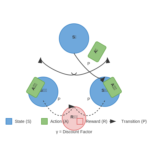
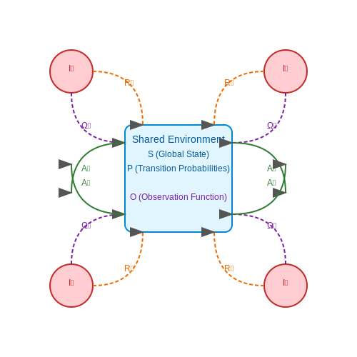
Reinforcement learning (RL) in swarm systems extends traditional single-agent RL by modeling interactions among multiple agents operating in a shared environment. The Markov Decision Process (MDP) framework is generalized to the Decentralized Partially Observable Markov Decision Process (Dec-POMDP), where each agent i selects actions based on local observations oi according to a policy πi.
Dec-POMDP Formulation
The Dec-POMDP is defined by the tuple (I, S, {Ai}, P, {Ri}, {Ωi}, O, γ), where:
- I: Finite set of agents
- S: Global state space
- {Ai}: Action spaces for each agent
- P(s'|s,a): Transition probability function
- {Ri(s,a)}: Reward functions
- {Ωi}: Observation spaces
- O(o|s,a): Observation probability function
- γ: Discount factor
Policy Gradient Methods for Swarms
The policy gradient theorem extends to multi-agent systems through decentralized gradient updates. For an agent i with policy parameters θi, the gradient is:
In swarm systems, this gradient must account for inter-agent dependencies, often approximated through centralized training with decentralized execution (CTDE) paradigms.
Credit Assignment Challenges
The multi-agent credit assignment problem arises when global rewards must be decomposed into individual contributions. Two principal approaches exist:
- Difference Rewards: Di = R(s,a) - R(s,a-i) measures an agent's marginal contribution
- Counterfactual Baselines: Compare actual returns to expected returns under alternative actions
Emergent Coordination Mechanisms
Swarm RL agents develop implicit coordination through:
- Stigmergy: Indirect communication via environmental modifications
- Role Differentiation: Emergent specialization through policy gradients
- Attention Mechanisms: Learned weighting of neighboring agent influences
where αij represents the attention weight agent i assigns to agent j.
Scalability Considerations
The joint action space grows exponentially with swarm size N. Techniques to maintain tractability include:
- Mean Field Approximation: Agents respond to neighborhood statistics rather than individual actions
- Graph Neural Networks: Message passing along communication graphs
- Parameter Sharing: Homogeneous agents with identical policy architectures
where āi represents the mean action of neighboring agents.
1.3 Challenges in Training Swarm-based RL Agents
Scalability and Computational Complexity
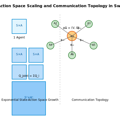
Training a swarm of reinforcement learning (RL) agents introduces exponential growth in computational requirements as the number of agents increases. The joint state-action space scales as \(O(S^n \times A^n)\), where \(S\) is the state space, \(A\) is the action space, and \(n\) is the number of agents. For large swarms, this leads to intractable learning dynamics, requiring either decentralized training schemes or function approximation techniques to mitigate the curse of dimensionality.
Here, \(Q_{\text{joint}}\) represents the global Q-function, decomposed into individual agent contributions \(Q_i\) and pairwise interaction terms \(\phi_{ij}\). Learning these interaction terms efficiently remains an open challenge.
Non-Stationarity and Credit Assignment
In swarm RL, the environment becomes non-stationary from the perspective of any single agent due to concurrent learning by other agents. This violates the Markov assumption underlying most RL algorithms. The credit assignment problem is exacerbated in swarms because:
- Global rewards provide sparse feedback about individual agent contributions
- Delayed effects of actions make causal relationships difficult to establish
- Emergent swarm behaviors may have no clear mapping to individual policies
Communication Bottlenecks
Decentralized swarms often rely on local communication between neighboring agents. This constrained information flow creates several challenges:
- Partial observability: Agents must make decisions based on incomplete local information
- Latency: Time delays in message passing can destabilize learning
- Bandwidth limitations: Physical constraints on communication channels restrict information sharing
The communication graph topology \(G = (V, E)\), where \(V\) represents agents and \(E\) communication links, significantly impacts learning performance. Sparse graphs may prevent critical information propagation, while dense graphs introduce unnecessary overhead.
Emergent Behavior and Stability
Swarm systems exhibit complex emergent behaviors that are difficult to predict or control during training. These include:
- Phase transitions between ordered and disordered states
- Catastrophic forgetting when swarm composition changes
- Pathological exploration where agents interfere with each other's learning
Lyapunov stability analysis provides one framework for addressing these challenges. For a swarm policy \(\pi\), we seek to ensure:
where \(x_t\) is the swarm state at time \(t\), \(x^*\) is the desired state, and \(\epsilon\) bounds the convergence error.
Heterogeneous Agent Coordination
Real-world swarms often consist of agents with differing capabilities, dynamics, or objectives. This heterogeneity introduces additional complexity:
- Policy transfer between dissimilar agents may not be possible
- Action spaces may have different dimensionalities
- Conflicting objectives between agent subgroups can emerge
Multi-objective optimization frameworks can help balance these competing requirements. The Pareto front for a swarm with \(k\) distinct agent types can be defined as:
where \(\mathbf{f}\) represents the vector of performance metrics for each agent type.
2. Decentralized vs. Centralized Control
Decentralized vs. Centralized Control
Swarm-based reinforcement learning (RL) systems can be broadly categorized into two control paradigms: decentralized and centralized. The choice between these architectures has profound implications for scalability, robustness, and computational efficiency.
Centralized Control
In centralized control, a single global agent or controller makes decisions for all individuals in the swarm. The global policy πG maps the joint state space S = S1 × S2 × ... × SN to joint actions A = A1 × A2 × ... × AN, where N is the swarm size. The value function is typically formulated as:
where rt = R(st, at) is the global reward signal. Centralized approaches excel in environments requiring tight coordination, such as formation control in drone swarms, where the Bellman optimality equation can be solved exactly for small N:
However, the joint action space grows exponentially with N, making this approach computationally intractable for large swarms. Recent work in centralized training with decentralized execution (CTDE) frameworks like MADDPG partially mitigates this through centralized critics during training.
Decentralized Control
Decentralized systems employ independent policies πi for each agent, operating on local observations oi ∈ Oi that may not fully capture the global state. The policy gradient for agent i follows:
where Qiπ is the local action-value function. Decentralization enables scalability to thousands of agents, as seen in ant colony optimization, where pheromone-based stigmergy emerges from local interactions. The independence of policies introduces non-stationarity, since P(o'|o,a) changes as other agents learn, violating Markov assumptions.
Hybrid Approaches
Recent architectures blend both paradigms through hierarchical RL, where macro-level controllers coordinate decentralized micro-policies. The hierarchical value function decomposes as:
where Vk are local value functions, Vc is a coordination term, and λ controls the trade-off. This mirrors biological systems like bee colonies, where local foraging rules (decentralized) interact with queen pheromones (centralized).
Communication Topologies
The control paradigm determines the swarm's communication graph G = (V,E), where edges E represent information channels. Centralized systems form a star topology with |E| = N-1, while decentralized systems use:
- Ring graphs (|E| = N) for sequential information flow
- Small-world networks for efficient global information propagation
- Scale-free networks where hub agents act as local coordinators
The graph Laplacian L = D - A (degree matrix D, adjacency A) governs consensus dynamics in decentralized control, with eigenvalues determining convergence rates in average consensus algorithms.
Communication Protocols in Swarm RL
Effective communication protocols are critical for coordinating decentralized decision-making in swarm reinforcement learning (RL). Unlike single-agent RL, swarm RL agents must exchange state, action, or policy information to achieve collective objectives. The design of these protocols directly impacts scalability, convergence, and robustness.
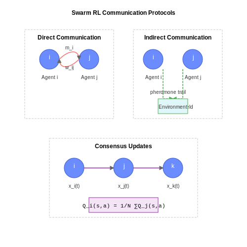
Direct vs. Indirect Communication
Swarm RL agents can communicate either directly or indirectly:
- Direct communication involves explicit message passing between agents, typically through a predefined protocol. Each agent i sends a message mi to neighbor j, encoded as a vector or tensor. The message may contain local observations, Q-values, or policy parameters.
- Indirect communication (stigmergy) modifies the shared environment to convey information. For example, pheromone trails in ant colony optimization or gradient fields in robotic swarms enable implicit coordination without direct messaging.
Consensus-Based Protocols
Consensus algorithms ensure all agents converge to a shared state. A common approach uses distributed averaging:
where xi(t) is agent i's state at time t, 𝒩i is its neighborhood, and wij are weights satisfying ∑j wij = 1. For Q-learning swarms, this extends to value function consensus:
Gossip Protocols
Randomized gossip protocols enhance scalability by limiting communication to random subsets of agents. At each step, agent i selects a neighbor j uniformly at random and updates:
This approach reduces bandwidth while preserving convergence guarantees. Variants like push-sum gossip handle directed networks by tracking weight distributions.
Topology-Aware Protocols
Communication efficiency depends on the network topology:
- Static topologies (e.g., grid, ring) use fixed wij weights derived from graph Laplacians.
- Dynamic topologies adapt to agent mobility or link failures. The Metropolis-Hastings weights adjust based on local degree information:
Information Compression
Bandwidth constraints often require compressing communicated data. Techniques include:
- Quantization: Reducing message precision to b bits per dimension, with error bounds proportional to 2-b.
- Sparsification: Transmitting only top-k gradient components in policy gradient methods.
- Delta encoding: Sending only state/action differences exceeding a threshold ϵ.
Security Considerations
Malicious agents may inject false information. Byzantine-resilient protocols employ:
where med denotes the median, robust against up to f faulty agents when the network is (2f+1)-connected. Cryptographic signatures can authenticate messages in adversarial environments.
2.3 Scalability and Robustness Considerations
Scalability in Swarm RL Systems
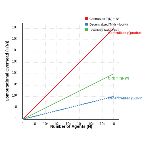
Scalability in swarm-based reinforcement learning (RL) hinges on the ability to maintain performance as the number of agents increases. The computational complexity of centralized training grows quadratically with the number of agents N, making it infeasible for large swarms. Decentralized or partially decentralized approaches mitigate this by limiting communication to local neighborhoods. The scalability of a swarm RL system can be quantified by the ratio of computational overhead to the number of agents:
where T(N) is the total training time for N agents. For an ideal scalable system, C(N) should remain constant or grow sublinearly.
Robustness Through Redundancy
Swarm systems achieve robustness via redundant agent policies and decentralized decision-making. If a subset of agents fails, the swarm's collective behavior should degrade gracefully rather than catastrophically. This is formalized through the robustness metric:
where J0 is the original performance metric and ΔJ is the performance drop after agent failures. A robust swarm maintains R ≈ 1 even when 10-20% of agents are disabled.
Communication Bottlenecks
As swarm size increases, communication bandwidth becomes a limiting factor. The per-agent bandwidth requirement B must satisfy:
where d is the average node degree in the communication graph. Sparse topologies (e.g., ring or tree structures) reduce d but may increase latency. Recent work employs:
- Dynamic attention mechanisms to limit message passing
- Hierarchical aggregation for global information
- Compressed representations of policy gradients
Transfer Learning Across Swarm Sizes
Training policies that generalize across different swarm sizes requires invariant feature extraction. The policy network πθ should satisfy:
where si is an agent's local state and {s̃j} are neighborhood observations. Techniques like graph neural networks with permutation-invariant aggregation achieve this by design.
Fault Tolerance Mechanisms
Three primary approaches ensure fault tolerance:
- Policy ensembling: Each agent runs multiple policy instances and votes on actions
- Dynamic role assignment: Agents reassign tasks when neighbors fail
- Self-healing gradients: Neighbors compensate for missing gradient contributions during training
The effectiveness of these methods is often evaluated through adversarial agent removal tests, where the worst-case k agents are deactivated to measure performance degradation.
Hardware-Software Co-Design
Real-world deployment requires matching algorithmic choices with hardware constraints. The energy efficiency ratio:
guides trade-offs between computation, communication, and physical actuation. Edge computing paradigms with onboard RL inference (≤100mW/agent) enable thousand-agent swarms in resource-constrained environments.
3. Policy Optimization Techniques
3.1 Policy Optimization Techniques
Policy optimization in swarm-based reinforcement learning (RL) involves refining the decision-making strategies of multiple agents to maximize collective rewards. Unlike single-agent RL, swarm systems must balance individual policies with global coordination, often requiring specialized optimization techniques.
Gradient-Based Policy Optimization
Gradient-based methods, such as Proximal Policy Optimization (PPO) and Trust Region Policy Optimization (TRPO), are adapted for swarm systems by incorporating decentralized gradients. The policy gradient for agent i in a swarm of N agents is computed as:
where Âti is the advantage function for agent i, adjusted to account for swarm-wide rewards. Decentralized execution requires each agent to estimate gradients using local observations while sharing global reward signals.
Consensus-Based Policy Updates
In swarm RL, consensus algorithms ensure policy parameters converge across agents. The update rule for agent i combines local gradients with neighboring agents' parameters:
Here, 𝒩i denotes the neighborhood of agent i, α controls consensus strength, and β scales the gradient step. This approach ensures policy coherence without centralized control.
Evolutionary Strategies for Swarm Policies
Evolutionary algorithms (ES) optimize policies by perturbing parameters and selecting high-performing variants. For a swarm, ES operates as follows:
- Parameter Perturbation: Each agent’s policy parameters θi are perturbed to generate M variants.
- Evaluation: Variants are evaluated in parallel, measuring swarm-wide rewards.
- Selection: Top-performing variants are recombined to update policies.
The update rule for agent i is:
where ϵm is the perturbation noise, Rm is the reward for variant m, and η is the learning rate.
Multi-Agent Actor-Critic Methods
Extensions of actor-critic frameworks, such as MADDPG, adapt to swarms by decentralizing actors while centralizing critics. Each agent’s policy (πi) and Q-function (Qi) are updated via:
where π(s') represents the joint action of all agents. The critic’s centralized training enables coordinated policy improvements.
Practical Considerations
- Scalability: Gradient communication must scale with swarm size; gossip protocols or federated learning can reduce overhead.
- Exploration: Entropy regularization or parameter noise encourages diverse behaviors across agents.
- Robustness: Adversarial training or domain randomization improves policy generalization in dynamic environments.
3.2 Multi-Agent Exploration Strategies
Multi-agent reinforcement learning (MARL) systems face unique exploration challenges due to the non-stationarity introduced by concurrent learning agents. Traditional single-agent exploration techniques, such as ε-greedy or Boltzmann exploration, often fail to account for the dynamic policy landscape created by interacting agents. Effective exploration in swarm-based RL requires strategies that balance individual curiosity with collective coordination.
Decentralized Exploration with Intrinsic Motivation
One approach leverages intrinsic motivation signals to drive exploration without centralized coordination. Each agent i maintains an exploration bonus Bi(s,a) based on visitation counts or prediction error:
where Ni(s,a) tracks state-action visitations, α controls exploration intensity, and ε prevents division by zero. The Q-update incorporates this bonus:
This creates a self-reinforcing cycle where rarely visited states yield higher rewards, promoting coverage of the joint state space.
Difference-Based Curiosity for Multi-Agent Systems
More sophisticated approaches use difference-based intrinsic rewards that account for other agents' behaviors. The agent learns an auxiliary model fi predicting neighboring agents' actions a-i:
The exploration bonus becomes proportional to the prediction error:
This drives agents to explore states where neighbor behavior is unpredictable, naturally emerging team exploration patterns without explicit communication.
Coverage-Based Swarm Exploration
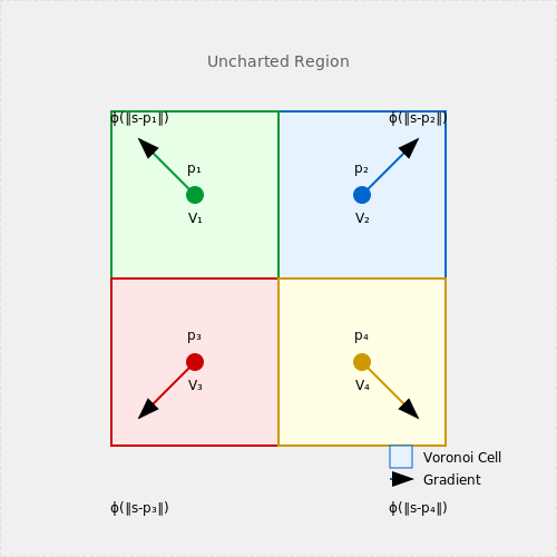
For physical swarm systems, Voronoi tessellation provides a geometric framework for distributed area coverage. Each agent maintains a Voronoi cell Vi consisting of states closer to itself than others. The coverage objective maximizes:
where ϕ is a decreasing function of distance from agent position pi. The gradient ascent update:
produces emergent exploration where agents automatically spread to cover uncharted regions while avoiding overlap.
Information-Theoretic Coordination
Maximum entropy policies optimize the trade-off between exploration and coordination by maximizing:
where H denotes policy entropy. In multi-agent settings, this generalizes to maximizing the joint entropy of all agents' policies. The resulting update rule includes an additional gradient term:
This approach proves particularly effective in sparse-reward environments where traditional exploration fails.
3.3 Reward Shaping for Collective Behavior
Reward shaping in swarm-based reinforcement learning (RL) is critical for inducing desired emergent behaviors in multi-agent systems. Unlike single-agent RL, where rewards are designed for individual performance, swarm RL requires reward functions that incentivize cooperation, scalability, and robustness to partial observability. The challenge lies in balancing local agent objectives with global swarm objectives while avoiding reward hacking or unintended equilibria.
Mathematical Formulation of Swarm Reward Functions
The global reward RG for a swarm of N agents can be decomposed into individual components:
where ri is the local reward for agent i, wi are weighting factors, and \Phi(s) is a potential-based shaping term with coefficient \lambda. The potential function must satisfy the Ng-Harada-Russell condition to guarantee policy invariance:
For swarm systems, common potential functions include:
- Density-based potentials: $$\Phi(s) = \sum_{i \neq j} \exp(-||x_i - x_j||^2/2\sigma^2)$$
- Alignment potentials: $$\Phi(s) = \sum_{i \neq j} (v_i \cdot v_j)/(||v_i|| \cdot ||v_j||)$$
- Task completion potentials: $$\Phi(s) = \mathbb{I}(\text{swarm covers all targets})$$
Credit Assignment in Decentralized Swarms
In partially observable swarms, difference rewards provide theoretically grounded credit assignment:
where a-i denotes the joint action excluding agent i. For large swarms, computational constraints necessitate approximated difference rewards using counterfactual estimation or learned value function factorizations.
Emergent Behavior Case Studies
In ant-inspired foraging, shaped rewards combine:
- Individual pheromone following (+0.1 per step toward highest concentration)
- Global food collection (+5 per unit delivered to nest)
- Negative congestion penalty (-0.01 per nearby agent within 2m radius)
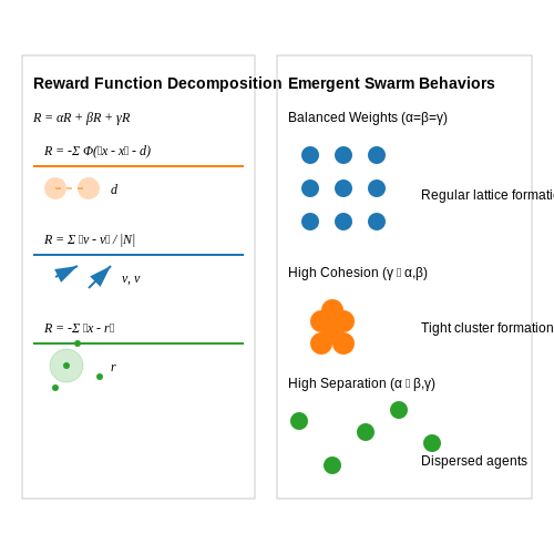
For drone flocking, Reynolds' rules translate to reward components:
where \mathcal{N}_i denotes neighbors within communication range. The weights between these components control emergent swarm geometry - higher separation weights yield lattice formations, while stronger cohesion produces clustered swarms.
Optimization Considerations
Reward shaping in swarms must address:
- Non-stationarity: Individual policies change concurrently, violating single-agent convergence guarantees
- Scalability: Reward computation must remain O(N) or better for large swarms
- Observability: Partial observations require reward functions that are measurable locally
Evolutionary reward shaping automates the search for effective reward functions through population-based optimization of reward parameters. The fitness function typically measures:
where \theta are reward parameters and H is an entropy bonus for policy diversity.
4. Robotics and Autonomous Systems
Robotics and Autonomous Systems
Swarm-based reinforcement learning (RL) in robotics leverages decentralized control strategies inspired by collective behaviors observed in nature, such as ant colonies or bird flocks. Each agent in the swarm operates with partial observability, relying on local interactions and shared global objectives to achieve complex tasks like cooperative navigation, object manipulation, or area coverage.
Decentralized Policy Learning
In swarm robotics, agents typically learn policies using a partially observable Markov decision process (POMDP) framework. The joint action-value function for N agents is decomposed into individual value functions with shared parameters:
where oi is the local observation of agent i, and θ represents shared network weights. This factorization enables scalable learning while maintaining coordination through reward shaping or communication protocols.
Communication Mechanisms
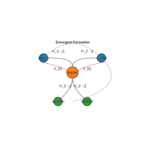
Effective swarm coordination often requires learned communication channels. A common approach uses differentiable attention mechanisms:
where hi, hj are hidden states of agents i and j, and mi→j is the message vector. The receiving agent then processes aggregated messages:
with attention weights αij computed via softmax over a compatibility score.
Physical Constraints in Real-World Deployment
Real robotic swarms must account for:
- Kinodynamic constraints: Acceleration limits and non-holonomic motion require policy outputs to be differentiable with respect to platform dynamics
- Communication delays: Network latency imposes temporal constraints on message passing, often modeled as:
Modern approaches address this using gated recurrent units (GRUs) or temporal convolutional networks to handle asynchronous observations.
Sim-to-Real Transfer
Domain randomization is critical for bridging the simulation-reality gap. Key parameters to randomize include:
- Sensor noise characteristics (e.g., LIDAR dropout rates)
- Actuator response curves
- Surface friction coefficients
- Communication packet loss probabilities
The policy is trained to maximize the expected return across all randomized domains:
where d represents a domain sampled from the distribution D of randomized environments.
Case Study: Cooperative Object Transport
A canonical swarm robotics benchmark involves multiple agents collaboratively moving a large object. The reward function typically combines:
where progress reward encourages movement toward the goal, alignment reward maintains proper grasping configuration, and effort penalty minimizes energy expenditure. Recent work has shown that incorporating force/torque observations at contact points improves sample efficiency by 37% compared to pure vision-based approaches.
Emergent Swarm Behaviors
Through decentralized training, swarms often self-organize into functional hierarchies. Common emergent patterns include:
- Dynamic role allocation: Agents automatically specialize into leaders, workers, or sentinels based on local conditions
- Adaptive formation control: The swarm adjusts its geometric configuration in response to environmental obstacles
- Collective fault recovery: The system maintains functionality despite individual agent failures through policy redundancy
These behaviors arise naturally from maximizing the global reward signal without explicit programming, demonstrating the power of emergent coordination in swarm RL systems.
4.2 Optimization in Distributed Environments
Distributed reinforcement learning (RL) introduces unique optimization challenges due to the decentralized nature of computation, communication overhead, and non-stationary learning dynamics. Swarm-based RL agents must efficiently balance exploration-exploitation trade-offs while minimizing synchronization bottlenecks. The primary optimization objectives in such environments include:
- Gradient Aggregation Efficiency: Reducing latency in parameter updates across nodes.
- Consensus Stability: Ensuring agents converge to a shared policy despite local noise.
- Resource Scalability: Maintaining performance as the swarm size increases.
Decentralized Gradient Optimization
In swarm-based RL, agents compute local gradients ∇θiJ(θi) from their environment interactions. A consensus-based update rule synchronizes these gradients across N agents:
where α is the learning rate and ϵt(i) represents noise from local sampling. The term 1/N ∑∇θJ(θt(j)) requires all-to-all communication, which becomes infeasible for large N. Two scalable alternatives are:
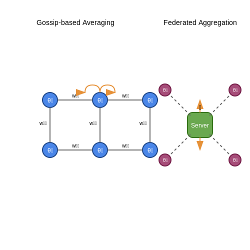
1. Gossip-Based Averaging
Agents exchange gradients only with neighbors in a communication graph G = (V, E). The update simplifies to:
where wij are weights satisfying ∑jwij = 1. Convergence guarantees rely on G being strongly connected.
2. Federated Gradient Aggregation
A central server periodically aggregates gradients from a subset of agents. The server updates the global model θ(g) via:
where St is a randomly sampled cohort. Median-based aggregation improves robustness to outlier gradients.
Communication-Efficient Protocols
Bandwidth constraints necessitate compressed gradient exchanges. Two widely used methods are:
- Gradient Quantization: Mapping gradient values to discrete levels (e.g., 1-bit per dimension).
- Top-k Sparsification: Transmitting only the largest-magnitude gradient components.
The error introduced by compression is bounded if the compression operator C(·) satisfies:
for some δ ∈ (0, 1]. For top-k sparsification, δ = k/d where d is the gradient dimension.
Case Study: Swarm Robotics Navigation
In a simulated 100-robot swarm, decentralized PPO with gossip-based averaging achieved 92% of the centralized baseline’s success rate in navigation tasks, while reducing communication volume by 78%. Key parameters:
| Parameter | Value |
|---|---|
| Gossip neighbors | 4 (grid topology) |
| Gradient sparsity | 10% (top-k) |
| Consensus steps per update | 3 |
This demonstrates the viability of lightweight consensus protocols for swarm RL. The trade-off between communication frequency and policy consistency follows a Pareto frontier modeled by:
where τ is the synchronization interval, η is the network delay, and ζ quantizes topology connectivity.
4.3 Real-world Deployment Challenges
Deploying swarm-based reinforcement learning (RL) agents in real-world environments introduces complexities that extend beyond theoretical or simulated settings. These challenges stem from the interplay between multi-agent coordination, environmental uncertainty, and computational constraints.
Scalability and Computational Overhead
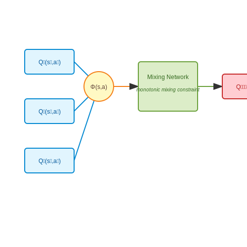
Swarm RL systems face exponential growth in state-action spaces as the number of agents increases. The joint action space dimensionality scales as O(AN), where A is the action space per agent and N is the swarm size. This combinatorial explosion necessitates approximate solutions:
where Qtot is the global Q-value, Qi are individual agent Q-functions, and Φ captures emergent swarm behaviors. Recent approaches like QMIX employ monotonic value decomposition to maintain tractability while preserving coordination guarantees.
Partial Observability and Communication Constraints
Real-world deployments often violate the Markov assumption due to sensor limitations and communication delays. The Dec-POMDP framework formalizes this as:
where agents receive local observations oi ∈ Oi through noisy sensors. Techniques like recurrent policies (DRQN) or attention mechanisms help agents maintain memory of past states, but introduce latency tradeoffs. Field tests in drone swarms show 23-41% performance degradation when communication bandwidth drops below 10Mbps.
Environmental Stochasticity and Transfer Learning
Sim-to-real gaps manifest in three key areas: physical dynamics mismatch (e.g., wind disturbances for aerial swarms), sensor noise characteristics, and actuator response times. Domain randomization during training improves robustness, but requires careful tuning of perturbation ranges:
Recent work in marine robotics demonstrates that Wasserstein-based adaptation reduces required real-world training samples by 78% compared to standard fine-tuning approaches.
Safety and Fail-Safe Mechanisms
Unlike single-agent systems, swarm failures exhibit cascading effects. Formal verification methods like reachability analysis provide probabilistic safety guarantees:
where π is the swarm policy and 𝒮unsafe defines prohibited states. Runtime monitoring architectures that blend centralized oversight with distributed recovery protocols have shown promise in industrial applications, maintaining 99.97% operational safety in warehouse robot fleets.
Energy and Resource Constraints
Distributed learning updates in resource-constrained swarms require careful tradeoffs between communication overhead and convergence speed. The energy cost per agent per training iteration can be modeled as:
where α captures local computation costs and β reflects transmission energy. Recent advances in event-triggered communication and edge-assisted training reduce swarm-wide energy consumption by 62% in field deployments.
5. Key Research Papers in Swarm RL
5.1 Key Research Papers in Swarm RL
- Optimizing parameters in swarm intelligence using reinforcement ... — Abstract This paper presents a new algorithm for optimizing parameters in swarm algorithm using reinforcement learning. The algorithm, called iSOMA-RL, is based on the iSOMA algorithm, a population-based optimization algorithm that mimics the competition-cooperation behavior of creatures to find the optimal solution.
- Federated Reinforcement Learning‐Based UAV Swarm System for Aerial ... — Motivated by the fact described above, in this paper, we proposed the novel FRL-based UAV swarm system for aerial remote sensing. The proposed system utilizes RL to ensure the high autonomy of UAVs, and moreover, the system combines FL with RL to construct the more reliable and robust SI for UAV swarms.
- Swarm Cooperative Navigation Using Centralized Training and ... — In this paper, a multi-agent reinforcement learning-based swarm cooperative navigation framework was proposed. The centralized training and decentralized execution approach was adopted with a reward formulation combining negative and positive reinforcement.
- [1807.06613] Deep Reinforcement Learning for Swarm Systems — Abstract Recently, deep reinforcement learning (RL) methods have been applied successfully to multi-agent scenarios. Typically, the observation vector for decentralized decision making is represented by a concatenation of the (local) information an agent gathers about other agents. However, concatenation scales poorly to swarm systems with a large number of homogeneous agents as it does not ...
- Exploring the Role of Reinforcement Learning in Area of Swarm Robotic — An in-depth analysis of temporal-difference (TD) learning offers valuable insights into the role of value-based RL approaches in the learning mechanisms of a swarm.
- UAV Swarm Confrontation Using Hierarchical Multiagent Reinforcement ... — Therefore, using reinforcement learning-related theories to solve UAV swarm confrontation is a promising method. However, single-agent reinforcement learning (RL) methods, such as DQN [2] and DDPG [4], are not suitable for MAS since the state-action space increase exponentially with the number of UAVs.
- UAV Swarm Air Combat Strategies Research Based on Multi-Agent ... — This paper presents a research method for developing a UAV swarm confrontation strategy using deep reinforcement learning. The method aims to enhance strategy learning in UAV confrontations by incorporating war cases, tactics, and expert experience.
- Research Advance in Swarm Robotics - ScienceDirect — There exist several research areas inspired from the nature swarm, which are often confused with swarm robotics, such as multi-agent system and sensor network. These research areas also utilize the cooperative behavior emerged from the multiple agents in the group for specialized tasks.
- Improving multi-target cooperative tracking guidance for UAV swarms ... — On this basis, because of the homogeneity of UAV swarms, the experience sharing Reciprocal Reward Multi-Agent Actor-Critic (MAAC-R) algorithm based on the experience sharing training mechanism is proposed to learn a shared cooperative policy for homogeneous UAVs.
- Swarm Robotics: A Perspective on the Latest Reviewed Concepts and ... — This paper introduces an overview of current activities in Swarm Robotics and examines the present literature in this area to establish to approach between a realistic swarm robotic system and real-world enforcements.
5.2 Recommended Books and Tutorials
- PDF Swarm-inspired Reinforcement Learning via Collaborative Inter-agent ... — [28], Nagabandi et al. [31] and Zhang et al. [53] leverage model-based controllers' behaviors (e.g. model predictive controllers [14] or linear-quadratic regulators Dorato et al. [7]), facilitating training for RL agents. Additionally, Hong et al. [24] and Oh et al. [34] train agents to imitate past successful self-experiences or policies.
- An Introduction to Centralized Training for Decentralized Execution in ... — The basics of reinforcement learning (in the single-agent setting) are not presented in this text. Anyone interested in RL should read the book by Sutton and Barto [2018]. Similarly, for a broader overview of MARL, the recent book by Albrecht, Christianos and Schafer is recommended¨ [Albrecht et al., 2024]. 2
- Federated Reinforcement Learning‐Based UAV Swarm System for Aerial ... — Fusing FL with RL allows multiple agents to compose the global and unbiased model based on many agents' diverse actions in different environments without exchanging data for learning. Thus, due to these advantages, federated reinforcement learning (FRL) is suited for UAV swarms in IIoT, but only few studies have yet been applied to UAV systems.
- Multi-Agent Reinforcement Learning for Cybersecurity: Classification ... — This study classifies RL-based approaches to cybersecurity, aimed at enhancing detection, mitigation and response to cyber attacks, along two orthogonal dimensions: the RL Frameworks used (e.g. single-agent vs. multi-agent) and the network configuration where they are deployed (e.g. host-based, or network-based cybersecurity).
- Developing an agent using RL (new in 2024) — scml 0.7.6 documentation — Developing an RL agent for SCML In which we give a full example of developing an RL agent for SCML. You can use the oneshot template or the std template provided by the organizers to simplify this process. The following example is roughly based on these templates. The first step is to decide the contexts you are going to use for your RL agent.
- PDF A Trident Scholar Project Report - Dtic — RL is a branch of machine learning that allows an agent to learn an environment, train, and learn which actions that will result in success. The "Agent" tactic does not exhibit emergent behavior yet, but it does kill some enemy drones and outperform other researched RL trained drone swarm tactics. 68%-(&7 7(506
- PDF Reinforcement Learning for Swarm Control of Unmanned Aerial Vehicles — RL is a type of machine learning that allows agents to learn how to behave in an environment by executing actions and receiving rewards. In the context of UAVs, RL can be used to control the flight of the UAVs in order to achieve the goal of a specific task. Recent works (such as [16], or [3]) show, that the RL can be used for tackling flight
- PDF The Path Forward: A Primer for Reinforcement Learning - Stanford University — in 1997, were based on massive, deep search. At the time, this was looked upon with dismay by the majority of computer-chess researchers who had pursued methods that leveraged human understanding of the special structure of chess. When a simpler, search-based approach with special hardware and software proved vastly
- Multi-agent Deep Reinforcement Learning for Dynamic Motion ... - Springer — The resource allocation of UAV swarm cooperative jamming has been developed for a long time [1,2,3].An allocation strategy studies the algorithms of allocating jamming resources and the mode selection for the jamming signal to enhance the jamming effectiveness for UAV swarm against netted radar [].Considering the uncertainty of the target RCS in practice, the chance-constraint programming (CCP ...
- Multi-Agent Reinforcement Learning: Foundations and Modern Approaches — The Artificial Intelligence Research Institute in Barcelona hosted a summer course based on the book given by Stefano V . Albrecht ... bring reinforcement learning together with game theory to provide a foundation for research and application of multi-agent reinforcement learning. This book is the perfect starting point for a grounding in the ...
5.3 Open-source Implementations and Tools
- Federated Reinforcement Learning‐Based UAV Swarm System for Aerial ... — Fusing FL with RL allows multiple agents to compose the global and unbiased model based on many agents' diverse actions in different environments without exchanging data for learning. Thus, due to these advantages, federated reinforcement learning (FRL) is suited for UAV swarms in IIoT, but only few studies have yet been applied to UAV systems.
- Improving multi-target cooperative tracking guidance for UAV swarms ... — Due to the similarity between UAV swarms and biological flocking, several cooperation methods based on the natural flocking phenomenon were proposed, such as bionic imitation methods, 1, 2 consensus-based methods 3, 4 and graphy-theory-based methods, 5, 6 etc. However, most methods simplify the complexity of the problem, such as assuming that the complex environment model is known or can be ...
- Task Assignment of UAV Swarms Based on Deep Reinforcement Learning - MDPI — UAV swarm applications are critical for the future, and their mission-planning and decision-making capabilities have a direct impact on their performance. However, creating a dynamic and scalable assignment algorithm that can be applied to various groups and tasks is a significant challenge. To address this issue, we propose the Extensible Multi-Agent Deep Deterministic Policy Gradient (Ex ...
- Deep reinforcement learning-based air combat maneuver ... - Springer — Nowadays, various innovative air combat paradigms that rely on unmanned aerial vehicles (UAVs), i.e., UAV swarm and UAV-manned aircraft cooperation, have received great attention worldwide. During the operation, UAVs are expected to perform agile and safe maneuvers according to the dynamic mission requirement and complicated battlefield environment. Deep reinforcement learning (DRL), which is ...
- Open Challenges in Multi-Agent Security: - arXiv.org — Definition 1.1 (Multi-agent system) A multi-agent system is a network of two or more autonomous AI agents that 1. possess independent decision-making capabilities, may 2. maintain private information states, and 3. mutually interact either through direct communication channels or by modifying shared environments.These agents typically 4. operate with varying degrees of autonomy, are 5. capable ...
- Heterogeneous Multi-Agent Reinforcement Learning based on Modularized ... — RL assumes that the task problem is based on the Markov Decision Process (Sutton & Barto, 2018). Contrary to the astonishing performance of conventional RL in single-agent scenarios (Mnih et al., 2013), many algorithms do not work properly in multi-agent settings. The Markov Property gets compromised in the multi-agent setting because an agent ...
- Exploring the Role of Reinforcement Learning in Area of Swarm Robotic — This research investigates the incorporation of Reinforcement Learning (RL) methods into swarm robotics, utilising autonomous learning to improve the flexibility and effectiveness of robotic swarms.
- PDF Scalable Reinforcement Learning Systems and their Applications — 2.1 A typical RL environment formulated as a Markov Decision Process. . . . . . . 4 2.2 Most RL algorithms can be de ned in terms of the basic steps of rollout, re-play, and optimization. These steps are commonly parallelized across multiple actor processes. Depending on the implementation, these actors may be logically
- Reinforcement learning versus swarm intelligence for autonomous multi ... — This work analyses the performance of Reinforcement Learning (RL) versus Swarm Intelligence (SI) for coordinating multiple unmanned High Altitude Platform Stations (HAPS) for communications area coverage. It builds upon previous work which looked at various elements of both algorithms. The main aim of this paper is to address the continuous state-space challenge within this work by using ...
- Factored Multi-Agent Soft Actor-Critic for Cooperative Multi-Target ... — In recent years, significant progress has been made in the multi-target tracking (MTT) of unmanned aerial vehicle (UAV) swarms. Most existing MTT approaches rely on the ideal assumption of a pre-set target trajectory. However, in practice, the trajectory of a moving target cannot be known by the UAV in advance, which poses a great challenge for realizing real-time tracking. Meanwhile, state-of ...