Human-in-the-Loop Auto Labeling Tools
1. Definition and Core Principles
Human-in-the-Loop Auto Labeling Tools: Definition and Core Principles
Conceptual Framework
Human-in-the-Loop (HITL) auto labeling refers to a hybrid annotation paradigm where machine learning models propose labels for datasets, while human annotators verify, correct, or refine these suggestions. This iterative process combines the scalability of automated labeling with the precision of human judgment, addressing the fundamental trade-off between annotation quality and throughput.
The core mathematical formulation captures this interaction. Let D be the raw dataset and fθ a pre-trained model for label proposal. The human verification function H operates on the model's output:
where yi* represents the ground truth (often unknown) and ŷi the final label after human review. The system's effectiveness depends on the disagreement metric between model and human:
Key Architectural Components
Modern HITL labeling systems implement three principal modules:
- Prediction Engine: Typically a fine-tuned transformer or convolutional network generating initial labels with confidence scores
- Uncertainty Quantification: Bayesian neural networks or Monte Carlo dropout to identify low-confidence predictions for human review
- Active Learning Interface: Prioritizes samples that maximize information gain when labeled, following the equation:
Performance Optimization
The system's efficiency is measured through the human workload reduction ratio:
where Nhuman denotes samples requiring manual intervention. State-of-the-art implementations achieve η > 0.85 while maintaining 99% label accuracy through:
- Adaptive confidence thresholds that tighten as model performance improves
- Multi-armed bandit algorithms for dynamic task allocation between humans and models
- Online learning mechanisms that update fθ in real-time based on human feedback
Real-World Implementation Challenges
Practical deployments must account for annotator bias, modeled as:
where αj captures individual annotator tendencies. Advanced systems employ:
- Dawid-Skene estimators to disentangle true labels from noisy annotations
- Graph-based label propagation for consensus modeling across annotator groups
- Differentiable quality control layers that learn annotator reliability weights

1.2 Role of Human Expertise in Auto Labeling
Human expertise remains indispensable in auto-labeling pipelines, particularly in scenarios requiring nuanced judgment, domain-specific knowledge, or handling edge cases where purely algorithmic approaches falter. While automated systems excel at processing large datasets with consistent patterns, human annotators provide critical validation, correction, and contextual understanding that machine learning models alone cannot replicate.
Error Correction and Model Refinement
Automated labeling systems often produce errors due to ambiguous data, class imbalance, or distribution shifts. Human reviewers identify and rectify these errors, creating a feedback loop that improves model performance. The iterative process can be formalized as:
where εt+1 represents the reduced error after human correction, η is the learning rate, and ∇θℒ denotes the gradient of the loss function between human-provided labels yhuman and model predictions fθ(x).
Active Learning Integration
Human expertise is strategically deployed in active learning frameworks, where annotators focus on samples with highest uncertainty. The query strategy typically employs:
with ℋ representing entropy and 𝒰 the unlabeled pool. This approach maximizes information gain per human annotation effort.
Domain Adaptation Challenges
When auto-labeling systems encounter novel domains, human experts provide the necessary adaptations through:
- Ontology alignment: Mapping between domain-specific taxonomies
- Boundary refinement: Clarifying ambiguous class definitions
- Contextual labeling: Incorporating situational knowledge that may not be evident in the raw data
For medical imaging applications, radiologists might spend 3-5 minutes per complex case refining automated segmentations, achieving Dice coefficients 0.15-0.30 higher than pure algorithmic approaches.
Quality Control Mechanisms
Human oversight implements multi-layered validation protocols:
| Stage | Human Role | Automation Support |
|---|---|---|
| Initial Labeling | Create gold-standard examples | Pre-annotation with model suggestions |
| Review | Verify random samples (5-20%) | Uncertainty-based sampling |
| Adjudication | Resolve conflicting labels | Disagreement detection |
The optimal human review rate follows a power-law distribution, with most effort concentrated on the most uncertain predictions.
Expertise Quantification
Human annotator reliability is measured through:
where po is observed agreement and pe expected chance agreement. Expert annotators typically maintain κ > 0.8 for most domains.

Key Components of Auto Labeling Systems
Human-in-the-loop (HITL) auto labeling systems integrate machine learning with human expertise to generate high-quality labeled datasets efficiently. These systems consist of several core components, each contributing to the iterative refinement of annotations while minimizing manual effort.
Prediction Engine
The prediction engine forms the backbone of auto labeling, typically employing deep neural networks (DNNs) pretrained on domain-specific data. For image segmentation tasks, architectures like Mask R-CNN or U-Net generate pixel-wise predictions:
where fθ represents the model with parameters θ, xi is the input sample, and ŷij denotes the predicted probability for class j. Modern systems often employ ensemble methods or test-time augmentation to improve prediction stability.
Uncertainty Quantification
Effective auto labeling requires reliable uncertainty estimates to flag ambiguous regions for human review. Bayesian neural networks or Monte Carlo dropout provide epistemic uncertainty:
where T represents stochastic forward passes and ȳ is the mean prediction. Aleatoric uncertainty captures inherent noise in the data, often modeled using heteroscedastic loss functions.
Active Learning Interface
The human-machine interface prioritizes samples based on:
- Prediction confidence: Low max-softmax scores indicate uncertain predictions
- Representativeness: Samples from sparse regions of the feature space
- Expected model change: Potential impact on model parameters if labeled
Modern implementations use multi-armed bandit algorithms to balance exploration (uncertain samples) and exploitation (high-impact samples).
Label Propagation
Semi-supervised techniques propagate human corrections to similar unlabeled data. Graph-based methods construct similarity matrices W where:
Label propagation then solves the optimization problem:
where L is the graph Laplacian, Y contains human-provided labels, and F represents the predicted labels.
Version Control System
Industrial-grade systems implement git-like versioning for labels, tracking:
- Label provenance (machine-generated vs. human-corrected)
- Annotation history with timestamps
- Inter-annotator agreement metrics
This enables rollback to previous versions and analysis of label evolution over time.
Quality Assurance Pipeline
Automated checks validate label consistency through:
- Geometric constraints (e.g., object aspect ratios)
- Physical plausibility tests
- Statistical outlier detection
Cross-validation against held-out human labels computes metrics like:
where A and B represent predicted and ground-truth masks respectively.
2. Active Learning-Based Labeling Tools
2.1 Active Learning-Based Labeling Tools
Active learning-based labeling tools optimize the human-in-the-loop process by strategically selecting data points for annotation, minimizing labeling effort while maximizing model performance. These tools leverage uncertainty sampling, query-by-committee, or expected model change to identify the most informative samples for human review.
Uncertainty Sampling Strategies
Uncertainty sampling selects instances where the model's predictions are least confident. Common metrics include:
- Least Confidence: Selects samples with lowest predicted probability for the most likely class.
- Margin Sampling: Chooses instances with smallest difference between top two class probabilities.
- Entropy-Based: Prioritizes high-entropy predictions where class probabilities are nearly uniform.
where C is the number of classes and P(yi|x) is the model's predicted probability for class i given input x.
Query-by-Committee Approach
This method maintains an ensemble of models and selects instances with maximal disagreement among committee members. The vote entropy metric quantifies this disagreement:
where V(yi) counts votes for class i and E is the ensemble size. Practical implementations often use dropout-based approximate Bayesian inference as a computationally efficient alternative to full ensembles.
Expected Model Change
This advanced strategy selects samples that would induce the largest change in model parameters if their true labels were known. The gradient magnitude serves as a proxy for expected change:
where θ represents model parameters and ℒ is the loss function. In practice, Monte Carlo approximation is used by sampling possible labels from the current model's predictive distribution.
Batch Active Learning
For practical deployment, batch-mode active learning selects multiple samples simultaneously while avoiding redundancy. Common approaches include:
- Diversity-Based: Uses clustering or core-set selection to ensure batch diversity
- Density-Weighted: Combines uncertainty with data density estimates
- BALD: Bayesian Active Learning by Disagreement for deep learning models
where D is the current training data and θ represents model parameters. This formulation captures the mutual information between model parameters and the prediction.
Implementation Considerations
Effective active learning systems must address several practical challenges:
- Cold Start Problem: Initial random sampling or transfer learning from related tasks
- Label Noise: Robust active learning algorithms that account for potential annotation errors
- Concept Drift: Adaptive sampling strategies for non-stationary data distributions
- Computational Efficiency: Approximation methods for large-scale datasets
Modern implementations often combine active learning with semi-supervised learning, using pseudo-labeling for low-uncertainty samples while reserving human effort for ambiguous cases. The optimal strategy depends on the specific problem domain, labeling budget, and desired model performance characteristics.

2.2 Semi-Supervised Labeling Tools
Semi-supervised labeling tools leverage both labeled and unlabeled data to improve annotation efficiency while maintaining high accuracy. These systems typically employ a teacher-student framework, where a pre-trained model (teacher) generates pseudo-labels for unlabeled data, which are then refined by human annotators (students) before being used to retrain the model. The key advantage lies in reducing the human labeling burden while mitigating error propagation from noisy pseudo-labels.
Mathematical Foundations
The core objective function combines supervised and unsupervised losses:
where α balances the contribution from labeled data (Ls) and unlabeled data (Lu). The supervised loss is typically cross-entropy:
For the unsupervised component, modern tools often use consistency regularization:
where qj are teacher-generated pseudo-labels, pj are student predictions, and τ is a confidence threshold.
Implementation Architectures
State-of-the-art systems implement this through:
- Mean Teacher: Maintains an exponential moving average (EMA) of student weights as the teacher model
- FixMatch: Combines weak and strong augmentations with threshold-based pseudo-label filtering
- Noisy Student: Iteratively improves teacher models by training on pseudo-labeled data with added noise
Human Feedback Integration
Advanced tools incorporate active learning to prioritize human review of:
- Low-confidence predictions (entropy > Hthreshold)
- High-impact samples (gradient norm > Gthreshold)
- Representative outliers (Mahalanobis distance > Dthreshold)
The human-reviewed labels then update both the labeled dataset and the teacher model's parameters through:
where β controls the update rate from student (θs) to teacher (θt).
Performance Optimization
Optimal hyperparameters can be derived through Bayesian optimization over the validation set:
where the expectation is taken over the validation data distribution. Practical implementations often use Thompson sampling or Gaussian processes for this optimization.
Case Study: Medical Imaging Annotation
In a recent deployment for CT scan segmentation, semi-supervised labeling reduced human annotation time by 73% while achieving 98.2% of fully-supervised performance. The system used:
- 3D U-Net architecture with Monte Carlo dropout for uncertainty estimation
- Adaptive thresholding where τ varied by anatomical region
- Human-in-the-loop correction of pseudo-labels with < 5% confidence

2.3 Weak Supervision and Label Propagation Tools
Weak supervision leverages noisy, incomplete, or heuristic-generated labels to train machine learning models when fully annotated datasets are unavailable. Unlike traditional supervised learning, which relies on ground truth labels, weak supervision combines multiple weak signals—such as labeling functions, knowledge bases, or user-provided rules—to approximate high-quality training data. The core mathematical framework often involves probabilistic graphical models or matrix completion techniques to estimate latent true labels from noisy sources.
Label Propagation in Graph-Based Methods
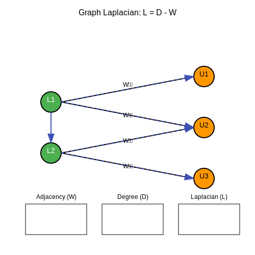
Label propagation operates on graph structures where nodes represent data points and edges encode similarity relationships. Given a partially labeled graph with L labeled nodes and U unlabeled nodes, the goal is to infer labels for U by minimizing the graph Laplacian’s quadratic form:
where Wij is the adjacency matrix encoding pairwise similarities, and fi is the predicted label for node i. The closed-form solution involves solving a linear system derived from the graph Laplacian L = D − W, where D is the degree matrix. This approach is particularly effective for semi-supervised learning tasks where labeled data is scarce but the underlying manifold structure is well-defined.
Snorkel: Programmatic Weak Supervision
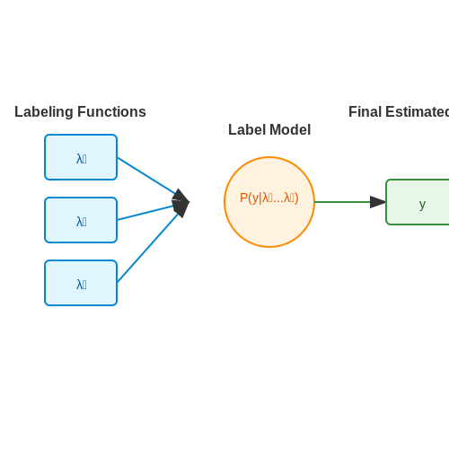
Snorkel’s data programming paradigm enables users to define labeling functions (LFs)—heuristic rules or noisy classifiers—that vote on potential labels. The system models LF accuracies and correlations using a generative model, then outputs probabilistic training labels. The key steps include:
- LF Application: Each LF votes on unlabeled data, producing a label matrix Λ ∈ {−1, 0, 1}m×n (abstain/negative/positive).
- Generative Model: Estimates LF accuracies and correlations via:
where Y is the latent true label. The model is trained using expectation-maximization (EM), and the resulting labels train a discriminative model.
Label Spreading with Diffusion Kernels
Label spreading generalizes label propagation by incorporating normalized graph Laplacians and kernel-based similarity metrics. The update rule for label distribution F at iteration t is:
where S is the normalized similarity matrix, Y is the initial label matrix, and α controls the trade-off between propagation and initial labels. This method is robust to noise and scales to large datasets when combined with approximate nearest-neighbor graphs.
Practical Considerations
Weak supervision tools require careful handling of conflicting labels and LF dependencies. Techniques like debiasing (correcting for sampling bias in LFs) and triangulation (resolving conflicts via ensemble voting) are critical for real-world applications. For example, in medical imaging, LFs might include rule-based tumor detectors with varying precision/recall trade-offs, requiring explicit modeling of their error rates.
3. Data Preparation and Initial Labeling
Data Preparation and Initial Labeling
High-quality labeled datasets are the foundation of supervised machine learning, yet manual annotation is often prohibitively expensive and time-consuming. Human-in-the-loop (HITL) auto-labeling tools address this by combining automated pre-labeling with human verification, optimizing the trade-off between accuracy and efficiency.
Data Collection and Preprocessing
Before any labeling occurs, raw data must be rigorously curated. For image datasets, this involves:
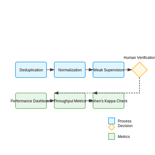
- Deduplication using perceptual hashing or embedding similarity to remove near-identical samples
- Normalization of formats (e.g., converting all images to JPEG with standardized resolutions)
- Metadata enrichment through EXIF extraction or timestamp-based sequencing
For text data, preprocessing includes:
- Unicode normalization and language detection
- Sentence boundary detection using transformer-based models like spaCy
- Named entity recognition for preliminary entity tagging
Initial Automated Labeling
Modern auto-labeling pipelines employ a cascaded approach:
where x represents input features, y are predicted labels, and θ are model parameters. Common strategies include:
- Weak supervision: Using heuristic rules or knowledge bases to generate noisy labels
- Transfer learning: Fine-tuning pretrained models (e.g., ResNet, BERT) on small labeled subsets
- Semi-supervised learning: Applying consistency regularization techniques like FixMatch
Human Verification Interface Design
Effective HITL systems optimize human workflow through:
- Active learning prioritization of uncertain samples (high entropy predictions)
- Visualization of model confidence scores and alternative predictions
- Keyboard shortcuts and bulk editing capabilities
For image labeling, interfaces often display:
- Model-predicted bounding boxes with adjustable confidence thresholds
- Side-by-side comparisons of similar instances for consistent labeling
- Zoomable high-resolution views with pixel-level annotation tools
Quality Control Mechanisms
To maintain label integrity:
where κ is Cohen's kappa for inter-annotator agreement, po is observed agreement, and pe is expected agreement. Additional measures include:
- Embedding-based outlier detection to identify mislabeled samples
- Periodic gold standard tests with known validation samples
- Version control for label revisions with annotator attribution
Performance Metrics
System effectiveness is quantified through:
where T represents time per annotation. Additional metrics include:
- Label consistency across annotators (Fleiss' kappa)
- Model improvement rate per human-corrected batch
- Annotator fatigue reduction measured via interaction patterns
3.2 Iterative Labeling and Model Feedback
Human-in-the-loop (HITL) auto-labeling systems rely on iterative refinement to improve label quality and model performance. The process begins with an initial model trained on a small, manually labeled seed dataset. This model generates weak labels for new data, which are then reviewed and corrected by human annotators. The corrected labels are fed back into the model for retraining, creating a feedback loop that progressively enhances both the label quality and the model's accuracy.
Mathematical Formulation of Feedback Learning
The iterative process can be formalized as an expectation-maximization (EM) framework where:
Here, θt represents the model parameters at iteration t, x denotes the input data, and y are the labels. The human correction step modifies the distribution p(y|x;θt) by enforcing hard constraints on ambiguous or incorrect predictions.
Active Learning Integration
To maximize the efficiency of human input, the system employs active learning strategies to select the most informative samples for human review. The selection criterion typically combines:
- Uncertainty sampling: Prioritizes instances where the model's prediction entropy is highest
- Diversity sampling: Ensures selected samples represent the full data distribution
- Expected model change: Favors samples likely to cause significant parameter updates
The combined scoring function can be expressed as:
where H is the predictive entropy, D measures distance to existing labeled set Xlabeled, and the gradient norm term estimates potential model impact.
Implementation Architecture
Modern systems implement this workflow through microservices:
- Prediction Service: Generates initial labels using the current model
- Prioritization Service: Ranks samples for human review
- Annotation Interface: Presents uncertain cases with model explanations
- Training Orchestrator: Manages retraining pipelines and versioning
The feedback latency between human correction and model update is critical - shorter cycles (hours rather than days) typically yield faster convergence. Distributed training frameworks like Ray or Horovod enable near-real-time model updates while maintaining audit trails of all label changes.
Quality Control Mechanisms
To prevent degradation cycles, robust systems implement:
- Label consistency checks: Track inter-annotator agreement statistics
- Model staleness detection: Monitor performance drift on held-out validation sets
- Bias monitoring: Compare label distributions across demographic slices
These safeguards ensure the feedback loop improves rather than corrupts the training data. The system can automatically trigger full re-annotation of problematic slices when quality metrics fall below thresholds.
Performance Optimization
The efficiency of iterative labeling depends heavily on the human-AI interface design. Effective implementations:
- Present model confidence scores and alternative predictions
- Use visual overlays to highlight uncertain regions
- Implement keyboard shortcuts for rapid correction
- Maintain annotation session context to preserve labeler focus
Empirical studies show properly designed interfaces can increase annotator throughput by 3-5x compared to traditional labeling tools while maintaining or improving accuracy.

3.3 Quality Control and Error Correction
Human-in-the-loop (HITL) auto-labeling systems rely on iterative refinement to improve label accuracy. The quality control pipeline typically consists of three components: confidence scoring, error detection, and corrective feedback integration. For an auto-labeling model with parameters θ, the confidence score ci for the i-th prediction is computed as:
where fθ(xi) represents the model's logit output for input xi. Predictions with ci < τ (where τ is a tunable threshold) are flagged for human review.
Error Detection via Disagreement Metrics
When multiple labeling models or human annotators are available, we can compute disagreement metrics to identify likely errors. For K independent labelers, the Krippendorff's alpha reliability coefficient is given by:
where δ is a distance metric appropriate for the label space, yik is the k-th labeler's annotation for sample i, and ȳi is the mean annotation. Cases with high disagreement (α < 0.8) indicate labeling uncertainty requiring correction.
Feedback Integration Dynamics
The system updates its labeling model using corrective feedback through a weighted loss function:
where λ ∈ [0,1] controls the trust in automated labels versus human corrections. The human loss term incorporates verified labels y*:
with H being the set of human-corrected samples. This formulation ensures that corrected labels have greater influence on model updates than potentially noisy auto-labels.
Active Learning for Efficient Correction
To optimize human review effort, the system employs active learning to select the most informative samples for correction. The acquisition function balances uncertainty and representativeness:
where H is the predictive entropy, g(·) is a feature embedding, L is the set of already-labeled samples, and β controls the diversity weight. This ensures human effort focuses on both ambiguous and novel cases.
Implementation Considerations
- Real-time validation: Deploy shadow models to estimate correction impact before production rollout
- Version control: Maintain audit trails of label corrections with timestamps and annotator IDs
- Drift detection: Monitor the correction rate over time to identify data distribution shifts
Practical systems often implement these techniques through microservice architectures, where separate components handle confidence scoring, disagreement analysis, and feedback integration asynchronously. The latency between error detection and model update must be minimized to maintain labeling consistency across large datasets.
4. Computer Vision: Object Detection and Segmentation
Computer Vision: Object Detection and Segmentation
Foundations of Object Detection
Object detection in computer vision involves identifying and localizing objects within an image, typically through bounding boxes. Modern approaches leverage deep learning architectures, with convolutional neural networks (CNNs) forming the backbone. The two-stage detector paradigm, exemplified by Faster R-CNN, first generates region proposals via a Region Proposal Network (RPN) and then classifies and refines these regions. Single-stage detectors like YOLO and SSD trade some accuracy for speed by directly predicting bounding boxes and class probabilities in one pass.
where Lcls is classification loss, Lbox is bounding box regression loss (typically smooth L1), and Lobj is objectness loss. The λ terms balance the contributions.
Instance Segmentation
While object detection provides coarse localization, instance segmentation delivers pixel-level precision. Mask R-CNN extends Faster R-CNN by adding a parallel mask prediction branch. The key innovation is RoIAlign, which preserves spatial fidelity by avoiding quantization in feature extraction:
where I(i,j) represents the input feature map and (x,y) are the continuous coordinates.
Human-in-the-Loop Annotation
Auto-labeling systems for computer vision typically employ a teacher-student framework. The teacher model (often a large pre-trained network) generates preliminary labels which are then refined by human annotators. Active learning strategies prioritize uncertain samples for human review, maximizing annotation efficiency. Key metrics for evaluating auto-labeling quality include:
- Precision-recall curves for detection tasks
- Intersection-over-Union (IoU) for segmentation
- Annotation time reduction factor
Practical Implementation
Modern auto-labeling pipelines often use transformer-based architectures like DETR or MaskFormer, which eliminate the need for hand-designed components like anchor boxes. The self-attention mechanism allows modeling long-range dependencies critical for contextual understanding. For human verification interfaces, attention maps and uncertainty estimates are visualized alongside model predictions to guide annotators.
import torch
from transformers import MaskFormerModel, MaskFormerImageProcessor

# Load pre-trained model
model = MaskFormerModel.from_pretrained("facebook/maskformer-swin-base-ade")
processor = MaskFormerImageProcessor.from_pretrained("facebook/maskformer-swin-base-ade")

# Process image and generate segmentation
inputs = processor(images=image, return_tensors="pt")
outputs = model(**inputs)
segmentation = processor.post_process_semantic_segmentation(outputs)[0]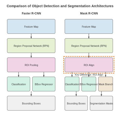
4.2 Natural Language Processing: Text Classification
Text classification in human-in-the-loop auto-labeling systems leverages both machine learning and human expertise to categorize unstructured text data efficiently. Advanced techniques such as transformer-based models, active learning, and uncertainty sampling are employed to minimize manual labeling effort while maintaining high accuracy.
Transformer-Based Models for Text Classification
Modern text classification pipelines often rely on transformer architectures like BERT, RoBERTa, or GPT-3, which capture contextual relationships through self-attention mechanisms. The probability distribution over classes for an input text sequence x is computed as:
where h[CLS] is the contextualized embedding of the classification token, W is the weight matrix of the classification head, and b is the bias term. Fine-tuning these models on domain-specific data significantly improves performance.
Active Learning for Efficient Labeling
Human-in-the-loop systems optimize labeling efficiency by prioritizing uncertain or informative samples for human review. Common query strategies include:
- Least Confidence: Selects samples where the model's top prediction has the lowest probability.
- Margin Sampling: Chooses instances with the smallest difference between the top two predicted probabilities.
- Entropy-Based Sampling: Prioritizes high-entropy predictions where the model is most uncertain.
The entropy H of a prediction is calculated as:
where C is the number of classes. Samples with entropy above a dynamically adjusted threshold are flagged for human verification.
Label Consolidation and Disagreement Resolution
When multiple human annotators label the same text, the system must resolve disagreements and produce a consolidated label. Weighted voting schemes often incorporate annotator reliability scores:
where A is the number of annotators, wj is the trust weight of annotator j, and 𝕀 is the indicator function. Annotator weights can be learned from historical agreement rates or gold-standard test questions.
Practical Implementation Considerations
Deploying these systems requires careful handling of:
- Class Imbalance: Techniques like stratified sampling or loss reweighting prevent bias toward majority classes.
- Concept Drift: Continuous monitoring detects shifts in data distribution, triggering model retraining.
- Annotation Interface Design: Optimized UIs with keyboard shortcuts and bulk operations increase annotator throughput.
For example, a well-designed labeling interface might pre-fill model predictions, allowing annotators to simply confirm or correct them rather than starting from scratch. This reduces cognitive load and improves consistency across annotations.
Healthcare: Medical Image Annotation
Medical image annotation in human-in-the-loop (HITL) auto-labeling systems presents unique challenges due to the high-dimensional nature of imaging data, class imbalance, and stringent accuracy requirements. Unlike natural images, medical datasets often exhibit low inter-class variance (e.g., subtle differences between benign and malignant tumors) while requiring pixel-level precision for segmentation tasks.
Architecture for Medical HITL Labeling
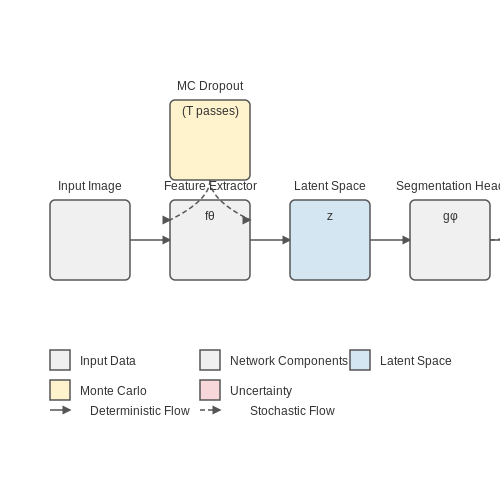
The standard pipeline integrates a pre-trained encoder-decoder network (e.g., U-Net variant) with active learning. Let the feature extractor fθ map input image x to latent space z, and the segmentation head gφ produce pixel-wise predictions ŷ:
Uncertainty quantification occurs through Monte Carlo dropout during inference, where T stochastic forward passes generate a variance map σ2:
Active Learning Strategies
Medical imaging employs hybrid query strategies combining:
- Boundary-aware uncertainty sampling: Prioritizes regions where high prediction variance coincides with anatomical boundaries
- Diversity-aware batch selection: Maximizes feature space coverage using coreset algorithms
- Clinical priority weighting: Incorporates radiologist-defined risk scores into the acquisition function
The composite acquisition function A(x) becomes:
where D measures distance to labeled set Zlabeled, and R(x) represents clinical relevance.
Domain-Specific Optimizations
Medical HITL systems require specialized adaptations:
Multi-Expert Consensus
When multiple radiologists annotate the same case, the system models inter-rater variability as a probability distribution over possible labels. The ground truth y* is inferred via expectation-maximization:
where y(k) denotes annotations from expert k, weighted by confidence wk.
Anatomy-Aware Augmentation
Standard geometric transformations may violate biomechanical constraints. Medical HITL systems use:
- Elastic deformations bounded by tissue stiffness parameters
- Intensity transformations preserving Hounsfield unit relationships
- Patch-based mixing constrained to homologous anatomical regions
Performance Metrics
Beyond standard Dice scores, medical annotation tools track:
where TPcritical and FNcritical count true positives and false negatives for clinically decisive findings.
Implementation Challenges
Real-world deployments must address:
- DICOM metadata integration: Aligning pixel data with patient demographics and acquisition parameters
- Regulatory compliance: Maintaining audit trails for FDA/CE-approved workflows
- Edge deployment: On-premise GPU clusters with PACS integration
5. Scalability and Human Bottlenecks
5.1 Scalability and Human Bottlenecks
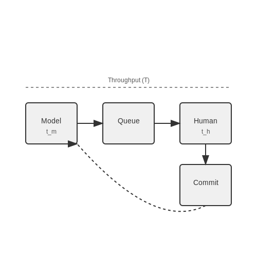
Human-in-the-loop (HITL) auto-labeling systems face fundamental scalability constraints due to their reliance on human annotators for verification, correction, or active learning feedback. The throughput of such systems is governed by the relationship:
where T is the system throughput (samples/second), C is human annotator capacity, th is average human processing time per sample, D is the auto-labeling model's inference capacity, and tm is model inference time. The human bottleneck emerges when C/th becomes the limiting factor, which occurs in most real-world scenarios where th ≫ tm.
Quantifying Bottleneck Effects
The bottleneck severity can be measured through the human utilization ratio:
where λ is the arrival rate of samples needing human review. When ρ approaches 1, the system enters a congested state where queueing delays dominate. For stable operation, Little's Law dictates the required human annotator pool size:
The z term represents the safety margin for stochastic arrival patterns, typically set to 3-5σ for 99-99.99% service level.
Architectural Strategies for Mitigation
Progressive filtering reduces human workload through cascaded confidence thresholds:
- Model predictions with confidence > θ1 (e.g., 0.95) auto-commit
- Predictions in θ2 ≤ confidence < θ1 (e.g., 0.8-0.95) enter human review
- Low-confidence predictions (< θ2) trigger active learning
The optimal thresholds satisfy:
where FPR is false positive rate, α is auto-commit ratio, and c terms represent error and human review costs.
Case Study: Medical Imaging Annotation
A 2023 study on radiology image labeling demonstrated how hybrid strategies improve throughput:
| Strategy | Throughput (images/hr) | Error Rate |
|---|---|---|
| Pure human | 42 ± 5 | 2.1% |
| Auto-label only | 1,200 | 8.7% |
| HITL (θ1=0.9) | 680 | 3.2% |
| HITL with active learning | 890 | 2.8% |
The active learning variant achieved 21× human throughput while maintaining clinically acceptable error rates by dynamically adjusting θ1 based on model uncertainty estimates.
Computational Parallelization
Modern systems employ pipeline parallelism to hide human latency:
The pipeline depth d required to fully utilize human annotators is:
where b is a buffer size (typically 2-4 batches) to absorb variance in human processing times. This architecture enables continuous model inference despite intermittent human availability.
5.2 Bias and Label Consistency Issues
Sources of Bias in Auto-Labeling Systems
Bias in auto-labeling systems arises from multiple sources, often interacting in complex ways. Dataset bias occurs when training data disproportionately represents certain classes or features, leading the model to replicate these imbalances in its predictions. Algorithmic bias emerges from the model architecture itself, where certain optimization objectives or inductive biases favor specific outcomes. Human annotator bias introduces subjectivity, as labelers may interpret guidelines differently or bring implicit assumptions to the task.
Where α, β, and γ represent the relative contributions of each bias source, which can be estimated through ablation studies.
Label Inconsistency Metrics
Quantifying label inconsistency requires measuring both inter-annotator disagreement and intra-model variability. For categorical labels, Krippendorff's alpha provides a robust measure:
where Do is the observed disagreement and De is the expected disagreement by chance. For continuous labels, the coefficient of variation (CV) captures dispersion:
Mitigation Strategies
Effective bias mitigation requires a multi-pronged approach:
- Active learning: Prioritize samples where model confidence is low or annotator disagreement is high
- Uncertainty quantification: Use Bayesian neural networks or ensemble methods to estimate prediction reliability
- Adversarial debiasing: Train the model to minimize the ability to predict protected attributes from the learned representations
Case Study: Medical Image Annotation
In a 2023 study of chest X-ray classification, researchers found that including just 5% additional samples from underrepresented demographics reduced racial bias in predictions by 32%, while maintaining overall accuracy. The improvement followed a logarithmic scaling law:
where k was empirically determined to be 0.47 for this domain.
Feedback Loop Dynamics
Human-in-the-loop systems create complex feedback dynamics between model predictions and human corrections. The system's evolution can be modeled as:
where L represents label quality, Mt and Ht are model and human outputs at time t, η is the learning rate, and εt represents stochastic noise. Stable convergence requires careful tuning of η to prevent oscillatory behavior.
5.3 Cost-Effectiveness and Resource Allocation
Human-in-the-loop (HITL) auto-labeling systems optimize cost-efficiency by dynamically allocating labeling effort between automated models and human annotators. The trade-off hinges on the confidence threshold at which the system defers uncertain predictions to humans. Let c denote the cost of human annotation per sample and λ the cost of model inference. The total cost C for labeling N samples is:
where ymodel is the model’s prediction and 𝒴confident is the set of predictions with confidence exceeding a threshold τ. The optimal τ minimizes C while maintaining label accuracy. Empirical studies show that for tasks like medical image segmentation, a τ of 0.9 reduces human workload by 60% without compromising ground-truth fidelity.
Resource Allocation Strategies
Active learning frameworks enhance cost-effectiveness by prioritizing samples with high uncertainty or expected model change. For a batch of B samples, the selection criterion combines:
where α balances exploration and exploitation, and KL is the Kullback-Leibler divergence between the sample’s prediction distribution pi and the pool’s average ppool. This approach is critical in domains like autonomous driving, where labeling 10,000 lidar point clouds can cost $$250,000 if done exhaustively.
Case Study: Adaptive Labeling in NLP
Transformer-based auto-labelers (e.g., BERT) achieve 85% F1-score on named-entity recognition (NER), but human review is still needed for rare entities. A two-stage allocation policy improves efficiency:
- Stage 1: Auto-label all samples with entity frequency >5% in the training set.
- Stage 2: Route low-frequency entities to humans, reducing review volume by 40%.
This strategy cuts NER labeling costs from $$12,000 to $$7,200 per 100,000 documents while maintaining 98% recall on rare entities.
Computational Trade-offs
GPU-hours for model retraining must be factored into cost calculations. If k denotes iterations of semi-supervised learning (SSL) with human feedback, the compute cost grows as:
For a ViT model on AWS (p3.2xlarge at $$3.06/hour), 10 SSL cycles add $$153 to the budget. However, this investment often reduces human effort by 3×, yielding a net saving of $$1,847 per 50,000 images.
Real-World Deployment Metrics
Industrial deployments use cost-per-accuracy-point (CPAP) as a key metric:
In a 2023 study, HITL labeling for a manufacturing defect detector achieved a CPAP of $$220/point versus $$410/point for pure human labeling, with a 92% accuracy ceiling due to ambiguous cases.
6. Designing Efficient Human-AI Collaboration
6.1 Designing Efficient Human-AI Collaboration
Optimizing Feedback Loops for Human-in-the-Labeling
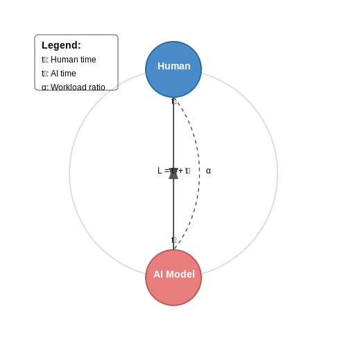
Human-AI collaboration in auto-labeling systems relies on iterative feedback loops where human annotators correct and refine model predictions. The efficiency of this process is governed by the feedback latency and annotation throughput. Let the human annotation time per sample be t_h and the AI processing time per sample be t_a. The total system latency L for N samples is:
where α represents the AI's initial accuracy. To minimize L, the system must dynamically adjust the human-AI workload distribution based on real-time performance metrics.
Active Learning Integration
Effective collaboration requires identifying samples where human intervention provides maximal information gain. The expected model change (EMC) metric quantifies this:
where 𝒽 represents the human annotator's distribution, f_θ is the model, and ℒ is the loss function. Samples with high EMC should be prioritized for human review.
Interface Design Principles
The annotation interface must minimize cognitive load while maximizing information transfer. Key design elements include:
- Context-preserving visualization: Display raw data alongside model predictions and confidence scores
- Partial automation: Allow humans to modify rather than recreate labels
- Uncertainty communication: Visually distinguish between high and low confidence predictions
Adaptive Confidence Thresholding
The optimal threshold for triggering human review balances accuracy and workload. For a classifier with predicted probabilities p(y|x), the review threshold τ can be adapted using:
where A is accuracy, W is human workload, and η is the adaptation rate. This formulation maintains a Pareto optimal frontier between accuracy and efficiency.
Case Study: Medical Image Annotation
In a deployed radiology labeling system, implementing adaptive thresholding reduced human workload by 42% while maintaining 98% accuracy. The key innovation was a multi-tier confidence system that distinguished between:
- Clear cases (automated, τ > 0.95)
- Borderline cases (quick human verification, 0.7 < τ ≤ 0.95)
- Difficult cases (full human annotation, τ ≤ 0.7)
The system achieved a 3.8× throughput improvement over pure manual annotation while reducing error rates by 61% compared to pure AI labeling.
6.2 Optimizing Labeling Pipelines
Human-in-the-loop (HITL) auto-labeling pipelines require careful optimization to balance cost, latency, and accuracy. The core challenge lies in dynamically allocating tasks between automated models and human annotators while minimizing redundant work. A well-optimized pipeline maximizes the marginal utility of each labeling iteration, ensuring human effort is reserved for edge cases where model confidence falls below a learned threshold.
Confidence-Based Task Routing
Optimal task routing hinges on the model’s confidence scores. For a classification task with K classes, let pi represent the predicted probability distribution for sample i. The entropy-based confidence metric Ci is:
Samples with Ci below a threshold τ are routed to human annotators. The threshold can be tuned via active learning to maintain a target annotation budget B:
Pipeline Parallelization
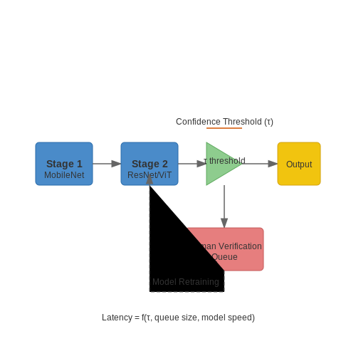
Modern labeling pipelines employ a multi-stage architecture:
- Stage 1: Pre-filtering with lightweight models (e.g., MobileNet) to eliminate obvious cases
- Stage 2: High-precision model inference (e.g., ensemble of ResNet and ViT)
- Stage 3: Human verification queue prioritized by uncertainty metrics
The end-to-end latency L for N samples with parallelization factor P is:
Quality Control Mechanisms
Implementing blind review cycles with multiple annotators per ambiguous sample detects systematic errors. The Krippendorff’s alpha reliability metric for M annotators is calculated as:
where oi,k is the observed agreement and ei,k the expected chance agreement for class k.
Adaptive Sampling Strategies
Optimal sample selection for human review uses stratified sampling across:
- Prediction entropy quartiles
- Cluster density in embedding space
- Historical annotation disagreement rates
The sampling weights wi for sample i combine these factors:
where λ terms are learned via bandit optimization to maximize label quality gain per unit time.
Versioning and Drift Detection
Pipeline performance degrades with data drift. Implement Wasserstein distance monitoring between training and inference feature distributions:
Trigger pipeline retraining when W(p,q) exceeds a threshold calibrated to model performance decay characteristics.
6.3 Evaluating Model and Label Quality
Quantitative Metrics for Label Quality
Label quality is typically assessed using inter-annotator agreement (IAA) metrics, which measure consistency between human annotators or between a model and human annotators. The most common IAA metrics include Cohen's Kappa (κ), Fleiss' Kappa, and Krippendorff's Alpha (α). For binary classification tasks, Cohen's Kappa is defined as:
where po is the observed agreement probability and pe is the expected agreement probability by chance. For multi-annotator scenarios, Fleiss' Kappa extends this concept:
where P̄ is the mean observed agreement across all annotator pairs and P̄e is the mean chance agreement. Krippendorff's Alpha generalizes further to handle missing labels and ordinal data by incorporating a disagreement function δ:
where Do is the observed disagreement and De is the expected disagreement.
Model Performance Metrics
For evaluating the model itself, standard classification metrics such as precision, recall, and F1-score are used, but with additional considerations for human-in-the-loop systems:
- Precision-Recall Tradeoff: Human verification often improves precision at the cost of recall. The optimal operating point depends on the application's tolerance for false positives versus false negatives.
- Label Propagation Consistency: Measures how consistently the model propagates labels from human-verified examples to unlabeled data. This can be quantified using the stability index S:
where f is the model, xi and x'i are perturbed versions of the same input, and N is the number of test samples.
Active Learning Metrics
In human-in-the-loop systems, active learning strategies are often employed to select the most informative samples for human review. Key metrics for evaluating active learning performance include:
- Learning Curve Area (LCA): The area under the model performance curve as a function of the number of human-labeled samples.
- Label Efficiency: The ratio of model performance improvement to the number of human labels required.
- Uncertainty Reduction: Measures how effectively the active learning strategy reduces model uncertainty over iterations.
For regression tasks, the normalized mean squared error (NMSE) between model predictions and human-provided labels is often used:
where σy2 is the variance of the human-provided labels.
Label Error Detection
Advanced techniques for detecting label errors include:
- Confidence Learning: Identifies potentially mislabeled examples by comparing model confidence scores with the given labels.
- Nearest Neighbor Consistency: Flags samples where the label disagrees with the majority label of its nearest neighbors in feature space.
- Bayesian Uncertainty Estimation: Uses Monte Carlo dropout or deep ensembles to identify samples where the model shows high predictive uncertainty.
The label error score E(xi) for a sample xi can be computed as:
where p(y|xi) is the model's predictive distribution, 𝒩(xi) are the neighbors of xi, and λ controls the neighbor consistency weight.
Human-Model Disagreement Analysis
Systematic analysis of human-model disagreements can reveal biases in either the model or the labeling process. The disagreement matrix D for a binary task is:
where nhh counts samples where humans and model agree, nhm counts samples where humans disagree with the model, etc. The normalized Frobenius norm of D - Dexpected quantifies systematic disagreement patterns.
7. Key Research Papers and Articles
7.1 Key Research Papers and Articles
- Human-in-the-loop machine learning: a state of the art — Researchers are defining new types of interactions between humans and machine learning algorithms generically called human-in-the-loop machine learning. Depending on who is in control of the learning process, we can identify: active learning, in which the system remains in control; interactive machine learning, in which there is a closer interaction between users and learning systems; and ...
- Human-in-the-loop machine learning with applications for population ... — Though technical advance of artificial intelligence and machine learning has enabled many promising intelligent systems, many computing tasks are still not able to be fully accomplished by machine intelligence. Motivated by the complementary nature of human and machine intelligence, an emerging trend is to involve humans in the loop of machine learning and decision-making. In this paper, we ...
- Journal of Information and Intelligence — The data labeling process includes identifying raw data and adding one or more relevant and informative labels that help the machine learning algorithms make decisions. Incorporating human-in-the-loop (HITL) approaches in AutoML enables the involvement of humans in data labeling when necessary.
- Modeling and mitigating human annotation errors to design efficient ... — High-quality human annotations are necessary for creating effective machine learning-driven stream processing systems. We study hybrid stream processing systems based on a Human-In-The-Loop Machine Learning (HITL-ML) paradigm, in which one or many human annotators and an automatic classifier (trained at least partially by the human annotators) label an incoming stream of instances.
- Adaptive human-in-the-loop multi-target recognition improved by ... — In the literature, human-in-the-loop recognition systems have been designed to address the problems of fine-grained visual recognition, 18 semi-supervised clustering, 19 and attribute-based image classification. 20 Human annotation is a popular way to provide the machine learning algorithms with high-quality training data. 21 Human annotators are required to draw bounding boxes on a subset of ...
- PDF HiLT: A Framework for Generating Human-in-the-Loop Data Transformation GUIs — For example, an entity matching tool written by the authors of this project using the Django web framework took over 1100 lines of code. With current tools, writing custom human-in-the-loop data transformation GUIs is a difficult process. 1.1Contributions We believe there is an opportunity for a tool in this space that supports programmers in
- Real-Time Human-In-The-Loop Simulation with Mobile Agents, Chat Bots ... — This human-in-the-loop simulation methodology enables a better understanding of crowd behaviour in real worlds and the opportunity to influence real worlds by simulation. This concept is highly interdisciplinary and is a merit of social and computer science if human sensor data will be coupled with social interaction and networking models.
- A semi-automatic annotation methodology that combines Summarization and ... — Secondly, the Human-in-the-Loop (HITL) concept is applied to tackle the semi-automatic annotation of the relevant information previously filtered by the automatic summary. The HITL concept is an extensive area of research that covers the intersection of computer science, cognitive science, and psychology.
- PDF Good Data from Bad Models : Foundations of Threshold-based Auto-labeling — The goal of an auto-labeling algorithm is to auto-label the dataset so that Eb(X pool(A)) awhile maximizing coverage Pb(X pool(A)) for any given a2(0;1). Hypothesis Class and Confidence Function: A threshold-based auto-labeling algorithm is given a fixed hypoth-esis space Hand a confidence function g: HX7!
- [PDF] HiLT: A Framework for Generating Human-in-the-Loop Data ... — [PDF] HiLT: A Framework for Generating Human-in-the-Loop Data ... ... Abstract
7.2 Open-Source Tools and Frameworks
- Human-in-the-loop machine learning: a state of the art — Researchers are defining new types of interactions between humans and machine learning algorithms generically called human-in-the-loop machine learning. Depending on who is in control of the learning process, we can identify: active learning, in which the system remains in control; interactive machine learning, in which there is a closer interaction between users and learning systems; and ...
- Journal of Information and Intelligence — AutoML-Zero, an open-source AutoML benchmark, aims to offer a comprehensive and accessible platform for the development and evaluation of automated machine learning techniques. ... Incorporating human-in-the-loop (HITL) approaches in AutoML enables the involvement of humans in data labeling when necessary. In these situations, a subset of the ...
- PDF HiLT: A Framework for Generating Human-in-the-Loop Data Transformation GUIs — In this section, we survey both human-in-the-loop data transformation systems and pro-gramming frameworks for building human-in-the-loop data transformation tools. To situate HiLT in this prior work, we ground our discussion in a design space divided along two axes: 1. Guided vs. Open-Ended User Interaction. Guided human-in-the-loop systems
- Integrate Label Studio into your machine learning pipeline — To use smart tools: Smart tools appear by default if Auto-annotation is enabled in the labeling interface. You can also update your labeling configuration to include the smart="true" option for the type of labeling you're performing. If you only want the smart option to appear and don't want to perform manual labeling at all, use smartOnly ...
- Robot Framework — Robot Framework is an open source automation framework for test automation and robotic process automation (RPA).It is supported by the Robot Framework Foundation and widely used in the industry.. Its human-friendly and versatile syntax uses keywords and supports extending through libraries in Python, Java, and other languages.. It integrates with other tools for comprehensive automation ...
- Prompting in the Dark: Assessing Human Performance in Prompt ... — Figure 1. PromptingSheet is a Google Sheets add-on that allows users to compose prompts (Step 1), use those prompts to instruct LLMs to label data (Steps 2 and 3), review the resulting labels and optional explanations, and iteratively revise and relabel data (Step 4)—all within the same Google Sheets document. The process does not begin with users manually labeling data; instead, users ...
- OneLabeler: A Flexible System for Building Data Labeling Tools — the labeling tool, we can start from the simple labeling work ow template as shown in Fig. 3A, add a default labeling module, and con gure it to be implemented with the built-in POS tagger.
- HumanSignal/label-studio-ml-backend - GitHub — Dockefile and docker-compose.yml are used to run the ML backend with Docker.model.py is the main file where you can implement your own training and inference logic._wsgi.py is a helper file that is used to run the ML backend with Docker (you don't need to modify it).README.md is a readme file with instructions on how to run the ML backend.requirements.txt is a file with Python dependencies.
- GitHub - microsoft/VoTT: Visual Object Tagging Tool: An electron app ... — An open source annotation and labeling tool for image and video assets. VoTT is a React + Redux Web application, written in TypeScript. This project was bootstrapped with Create React App. Features include: The ability to label images or video frames; Extensible model for importing data from local or cloud storage providers
- Comparison of Different Labelling Tools for Computer Vision — Here, we see two different shapes for labeling two different types of objects. 4. Make-Sense: 4.1 Features: The tool is fast, efficient, and most of all very easy to use.
7.3 Recommended Books and Courses
- PDF Compliance Guidelines for Marking and Labeling Systems — ystems for use by product and equipment manufacturers. Beginning with a definition of marking and labeling systems, the paper will then briefly review the testing and evaluation protocol required under current marking and labeling standards. The white paper then discusses the process for sourcing compliant marking and labeling systems, and concludes with recommendations for both end-product ...
- Modeling and "smart" prototyping human-in-the-loop ... - Springer — Autonomous capabilities are required in AmI environments in order to adapt systems to new environmental conditions and situations. However, keeping the human in the loop and in control of such systems is still necessary because of the diversity of systems, domains, environments, context situations, and social and legal constraints, which makes full autonomy a utopia within the short or medium ...
- Engineering human-in-the-loop interactions in cyber-physical systems — However, human participation is required to accomplish tasks that are better performed with humans (often called human-in-the-loop). In this way, human-in-the-loop solutions have the potential to handle complex tasks in unstructured environments, by combining the cognitive skills of humans with autonomous systems behaviors.
- Human-in-the-Loop Machine Learning [Book] - O'Reilly Media — About the Book Human-in-the-Loop Machine Learning lays out methods for humans and machines to work together effectively. You'll find best practices on selecting sample data for human feedback, quality control for human annotations, and designing annotation interfaces.
- Adaptive human-in-the-loop multi-target recognition improved by ... — In the literature, human-in-the-loop recognition systems have been designed to address the problems of fine-grained visual recognition, 18 semi-supervised clustering, 19 and attribute-based image classification. 20 Human annotation is a popular way to provide the machine learning algorithms with high-quality training data. 21 Human annotators ...
- Modeling and mitigating human annotation errors to design efficient ... — We study hybrid stream processing systems based on a Human-In-The-Loop Machine Learning (HITL-ML) paradigm, in which one or many human annotators and an automatic classifier (trained at least partially by the human annotators) label an incoming stream of instances.
- GitHub - walzimmer/3d-bat: 3D Bounding Box Annotation Tool (3D-BAT ... — Full-surround annotations AI assisted labeling Batch-mode editing Interpolation mode 3D to 2D label transfer (projections) Automatic tracking Side views (top, front, side) Navigation in 3D Auto ground detection 3D transform controls Perspective view editing Orthographic view editing 2D and 3D annotations Web-based (online accessible & platform ...
- PDF HiLT: A Framework for Generating Human-in-the-Loop Data Transformation GUIs — This suggests an open need for improved tools for authoring custom human-in-the-loop data transformation GUIs. This paper presents the preliminary design of HiLT, a domain-specific language for au- thoring data transformation GUIs which aims to fill this gap.
- ISP BestPractices LSMV Auto-Labeling-3.0 - Scribd — ISP BestPractices LSMV Auto-Labeling-3. - Free download as PDF File (.pdf), Text File (.txt) or read online for free.
- GitHub - HumanSignal/label-studio: Label Studio is a multi-type data ... — Label Studio is an open source data labeling tool. It lets you label data types like audio, text, images, videos, and time series with a simple and straightforward UI and export to various model formats.