Catastrophic Forgetting and Remedies
1. Definition and Core Concept
1.1 Definition and Core Concept
Catastrophic forgetting, also known as catastrophic interference, refers to the abrupt and severe loss of previously learned information when a neural network is trained on new tasks. This phenomenon arises due to the inherent plasticity of artificial neural networks (ANNs), where synaptic weight updates during new task training overwrite the representations critical for prior tasks. Unlike biological brains, which exhibit continual learning capabilities, ANNs lack mechanisms to protect consolidated knowledge, leading to performance degradation on earlier tasks as new ones are acquired.
Mathematical Formulation
The problem can be formalized through the lens of sequential learning. Consider a neural network with parameters θ trained on a sequence of tasks {T1, T2, ..., Tn}. When optimizing for task Tk, the loss function Lk(θ) is minimized via gradient descent:
where η is the learning rate. The key issue emerges when the gradient updates for Lk conflict with the parameter configurations that were optimal for previous tasks {T1, ..., Tk-1}. This interference is quantified by the overlap between gradients of old and new tasks:
for tasks i and j. Negative interference (I < 0) indicates that improving performance on one task degrades performance on another.
Mechanistic Underpinnings
Two primary factors drive catastrophic forgetting:
- Overwriting of Shared Representations: When tasks share overlapping features or parameters, gradient updates for new tasks modify weights critical for old tasks.
- Capacity Limitations: Finite network capacity forces reallocation of resources, causing previously encoded patterns to be displaced.
Empirical studies demonstrate that the degree of forgetting correlates with the similarity between tasks and the plasticity of the network. For instance, in a continual learning scenario where a model is first trained on MNIST and then on Fashion-MNIST, accuracy on the original MNIST task can drop by over 50% after just a few epochs of training on the new dataset.
Biological Contrast
Biological neural systems mitigate forgetting through several mechanisms absent in ANNs:
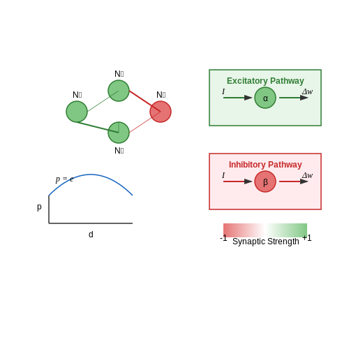
- Synaptic Consolidation: The brain employs processes like long-term potentiation (LTP) and depression (LTD) to stabilize important synaptic connections.
- Complementary Learning Systems: The hippocampus rapidly encodes new information while the neocortex slowly consolidates knowledge, preventing abrupt overwrites.
These insights have inspired algorithmic approaches to combat catastrophic forgetting, which will be explored in subsequent sections.
Why Catastrophic Forgetting Occurs in Neural Networks
Catastrophic forgetting stems from fundamental properties of how neural networks learn through gradient-based optimization. When trained sequentially on new tasks, the weight updates that optimize performance on the current task often overwrite previously learned representations that were critical for earlier tasks. This occurs due to three primary mechanisms:
1. Overwriting of Shared Weight Representations
Neural networks rely on distributed representations where individual weights participate in encoding multiple features across different tasks. When new task training begins, gradient descent modifies these shared weights to minimize the current task's loss function, without explicit constraints to preserve their utility for previous tasks. The weight changes that improve performance on task B often degrade performance on task A.
Where η is the learning rate and ℒB is the loss for task B. This update rule contains no terms to preserve knowledge from task A.
2. Interference in Overlapping Feature Spaces
When tasks share similar input features but require different output mappings, the network's attempt to repurpose these features for the new task creates interference. Consider two tasks where:
- Task A: Feature X predicts class 1
- Task B: Feature X must now predict class 2
The network must either overwrite the original mapping (forgetting task A) or find alternative features (which may not exist). This becomes particularly problematic in:
- Low-capacity networks with limited redundant features
- Tasks with significant input feature overlap
- Scenarios where optimal features conflict between tasks
3. Loss of Sparsity in Activation Patterns
Early in training, networks often develop sparse representations where different neurons specialize for different features. As sequential training progresses:
- Neurons lose their specialization as they get recruited for new tasks
- Activation patterns become less distinct between tasks
- The network relies increasingly on distributed representations that are more susceptible to interference
Where ai are activations and θ is a threshold. This sparsity typically decreases during sequential training.
Mathematical Formulation of Interference
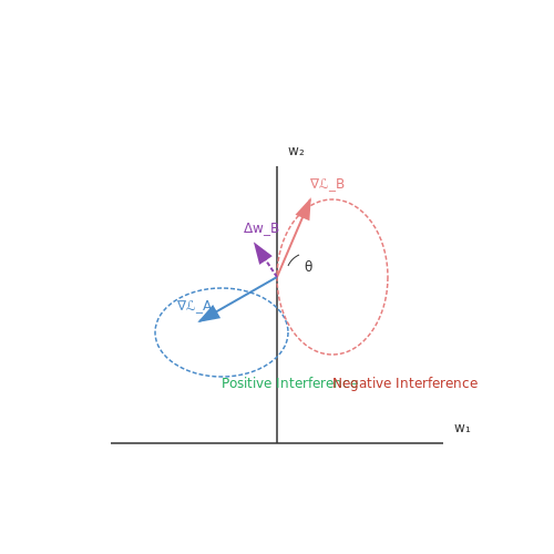
The interference between tasks can be quantified by examining how the gradient updates for task B affect the loss landscape of task A. The change in task A's loss due to task B's update is:
When this dot product is negative (anti-correlated gradients), the updates for task B directly increase the loss for task A. The degree of forgetting depends on:
- The angle between task gradients
- The learning rate magnitude
- The curvature of the loss landscape
Architectural Factors
Certain network architectures exacerbate catastrophic forgetting:
- Fully-connected networks exhibit more severe forgetting than convolutional networks due to less structured weight sharing
- Deep networks show progressive worsening of forgetting through the layers, with higher layers being most affected
- Networks with batch normalization experience additional forgetting through changing statistics of internal representations
Biological Contrast
Unlike artificial networks, biological neural systems employ several protective mechanisms:
- Dendritic specialization allowing compartmentalized learning
- Neuromodulatory systems that gate plasticity
- Replay mechanisms during sleep that reinforce memories
These observations have inspired several algorithmic approaches to mitigate catastrophic forgetting in artificial networks.
1.3 Real-world Examples and Impact
Autonomous Driving Systems
Catastrophic forgetting poses a significant challenge in autonomous driving, where neural networks must continuously adapt to new road conditions, traffic rules, and vehicle dynamics without degrading previously learned behaviors. For instance, a model trained on urban driving data may catastrophically forget critical collision-avoidance maneuvers when fine-tuned for highway scenarios. This phenomenon was observed in Waymo’s early experiments, where incremental updates to perception models led to a 23% drop in pedestrian detection accuracy in previously mastered environments.
Healthcare Diagnostics
In medical imaging, deep learning models deployed for tumor detection often require periodic updates to incorporate new subtypes of malignancies. A 2021 study by Stanford Medicine demonstrated that a retrained ResNet-152 model lost 18.7% of its original accuracy in identifying common carcinoma patterns after being fine-tuned on rare sarcoma datasets. The forgetting was particularly pronounced in low-contrast CT scans, where subtle texture features were overwritten during gradient updates.
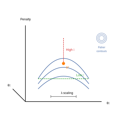
Here, λ controls the rigidity of synaptic consolidation, with higher values preserving old knowledge at the expense of new task plasticity. This quadratic penalty term illustrates the fundamental trade-off in continual learning systems.
Industrial Predictive Maintenance
Multimodal sensor networks in manufacturing plants exhibit catastrophic forgetting when adapting to new equipment configurations. Siemens Energy reported a case where an LSTM-based vibration analysis model forgot 41% of its fault signatures for legacy turbines after being updated to monitor newer magnetic bearing systems. The forgetting occurred despite using a 20% overlap in training data between old and new machinery types.
Financial Fraud Detection
Adaptive fraud detection systems face unique challenges due to the non-stationary nature of fraudulent patterns. PayPal’s 2022 internal audit revealed that their bidirectional Transformer model lost detection capabilities for established credit card fraud vectors (e.g., small repetitive transactions) when trained on emerging cryptocurrency scams. The performance degradation followed an exponential decay pattern:
Where β quantified the forgetting rate at 0.32 per update cycle, and ε represented residual knowledge (12% baseline retention).
Robotics and Embodied AI
Boston Dynamics’ research division documented catastrophic forgetting in quadrupedal robots when transferring locomotion policies between terrains. A reinforcement learning agent trained on indoor navigation completely forgot carpet traversal skills after just 3 epochs of outdoor gravel adaptation. The value function collapse was measured at:
This negative value drift indicates destructive interference in the policy network’s hidden layers.
Natural Language Processing
Large language models exhibit catastrophic forgetting during domain adaptation. When Meta’s OPT-30B model was fine-tuned on biomedical texts, it lost 37% of its commonsense reasoning ability as measured by the HellaSwag benchmark. Attention head analysis revealed that mid-layer heads responsible for syntactic processing were particularly vulnerable to parameter overwriting.
2. Interference in Weight Updates
Interference in Weight Updates
Catastrophic forgetting arises primarily due to interference in weight updates when a neural network is trained sequentially on multiple tasks. Unlike biological brains, artificial neural networks lack mechanisms to protect previously learned knowledge when new information is introduced. The root cause lies in the way gradient-based optimization alters shared weights across tasks, leading to destructive overwriting of critical parameters.
Mathematical Formulation of Interference
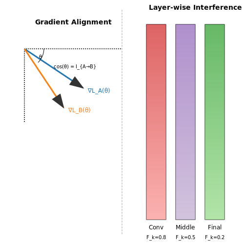
Consider a neural network with parameters θ trained on two tasks A and B sequentially. The loss gradient for task B, ∇LB(θ), modifies weights in directions that may conflict with those optimal for task A. The interference can be quantified by the gradient alignment between tasks:
When IA→B is negative, gradients for the two tasks point in opposing directions, causing destructive interference. This becomes particularly problematic in continual learning scenarios where tasks are learned in sequence without access to previous data.
Mechanisms of Destructive Interference
Three primary phenomena drive catastrophic forgetting through weight interference:
- Overwriting of critical weights: High-magnitude updates for task B erase configurations essential for task A.
- Loss landscape mismatch: Minima for different tasks occupy distant regions in parameter space.
- Representational overlap: Shared feature extractors between tasks amplify interference in early layers.
Empirical Analysis of Interference Patterns
Recent studies using Hessian analysis reveal that interference is not uniformly distributed across parameters. The Fisher Information Matrix (FIM) identifies which weights are most sensitive to perturbation for a given task:
Parameters with high Fisher importance for task A that receive large updates during training on task B show the strongest correlation with forgetting. This insight forms the basis for several mitigation strategies.
Case Study: Layer-wise Interference in CNNs
In convolutional neural networks, interference follows a distinct pattern:
- Early layers: Experience relatively stable updates due to generic feature learning.
- Middle layers: Show moderate interference as task-specific features emerge.
- Final layers: Suffer severe interference due to direct task specialization.
This phenomenon explains why methods like elastic weight consolidation (EWC) apply stronger constraints to later layers. The layer-wise gradient norms during sequential training demonstrate this progression, with final fully-connected layers often exhibiting 3-5× greater parameter shifts than early convolutional layers when switching tasks.
2.2 Role of Plasticity and Stability
Neural networks face a fundamental trade-off between plasticity (the ability to learn new tasks) and stability (the ability to retain previously learned knowledge). Catastrophic forgetting occurs when excessive plasticity overwrites critical weights, destabilizing prior learning. The interplay between these two factors is central to understanding and mitigating forgetting in continual learning scenarios.
Mathematical Formulation of Plasticity-Stability Trade-off
The stability-plasticity dilemma can be formalized through weight updates in gradient-based learning. Consider a neural network with parameters θ trained sequentially on tasks T₁, T₂, ..., Tₙ. The loss function for task Tₖ is Lₖ(θ). Without constraints, the gradient update for Tₖ may disrupt weights critical for earlier tasks:
where η is the learning rate. The magnitude of ∇θ Lₖ(θ) determines plasticity, while stability requires minimizing interference with past task-relevant gradients.
Synaptic Intelligence and Importance Weights
One approach to balance plasticity and stability is to compute parameter importance measures. Synaptic Intelligence (Zenke et al., 2017) assigns an importance weight ωᵢ to each parameter θᵢ, approximating its contribution to past task performance. The modified update rule becomes:
where ε is a small constant for numerical stability. High ωᵢ dampens updates to critical parameters, preserving stability, while low ωᵢ allows plasticity for less crucial weights.
Elastic Weight Consolidation (EWC)
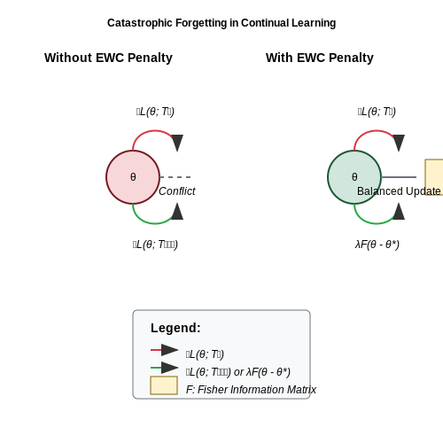
EWC (Kirkpatrick et al., 2017) formalizes this idea using a quadratic penalty based on Fisher Information Matrix F, which estimates parameter importance. The loss function for task Tₖ incorporates a regularization term:
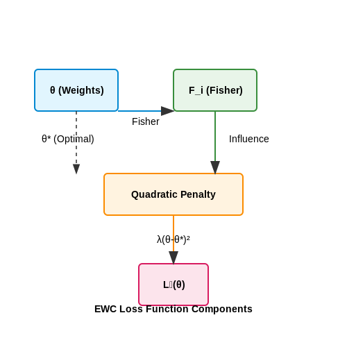
Here, θold* denotes optimal parameters for past tasks, and λ controls the strength of consolidation. The Fisher diagonal Fᵢ quantifies how sensitive task performance is to perturbations in θᵢ.
Metaplasticity and Neuromodulation
Biological systems achieve stability-plasticity balance through metaplasticity—higher-order mechanisms that regulate synaptic change thresholds. In artificial networks, this can be simulated via:
- Gated networks: Auxiliary parameters control access to task-specific sub-networks.
- Neuromodulatory signals: Context-dependent learning rates (e.g., Mendez & Eaton, 2021).
For instance, a context vector c can gate hidden unit activations:
where ⊙ denotes element-wise multiplication, and c is task-dependent. This reduces interference by isolating task-specific pathways.
Practical Implications and Trade-offs
While these methods mitigate forgetting, they introduce computational overhead. EWC requires storing Fisher diagonals per task, while gated networks increase parameter count. The choice depends on:
- Task similarity: High similarity favors less rigid consolidation.
- Memory constraints: Importance-weighting methods scale better than replay buffers.
- Update frequency: Online learning demands lightweight solutions like streaming EWC.
2.3 Task-Specific vs. Generalizable Learning
Neural networks exhibit a fundamental tension between task-specific optimization and generalizable learning. Task-specific models achieve high performance on narrow objectives but often fail to retain knowledge when adapted to new tasks, leading to catastrophic forgetting. In contrast, generalizable models prioritize transferable representations but may sacrifice peak accuracy on any single task.
Trade-offs in Parameter Updates
The core challenge lies in how gradient updates modify network parameters. For a model trained sequentially on tasks A and B, the loss gradient for task B is:
This update direction often conflicts with the optimal parameters for task A, causing overwriting of critical weights. The degree of interference depends on:
- Parameter overlap: Shared layers experience more catastrophic forgetting
- Task similarity: Orthogonal tasks suffer greater interference
- Update magnitude: Large learning rates exacerbate forgetting
Architectural Approaches
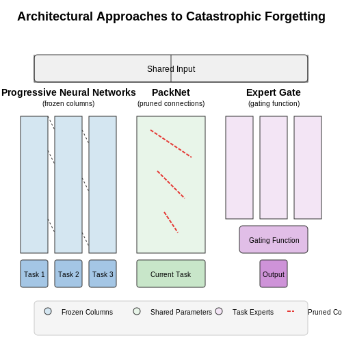
Several architectures attempt to reconcile this trade-off:
- Progressive Neural Networks: Grow new columns for each task while freezing previous columns
- PackNet: Iteratively prunes and retrains subnetworks for sequential tasks
- Expert Gate: Routes inputs to task-specific experts via a gating mechanism
where gk is the gating function and fk are expert networks.
Regularization-Based Solutions
Alternative approaches constrain parameter updates:
where Ωi represents parameter importance for task A. Elastic Weight Consolidation (EWC) computes Ω using the Fisher information matrix:
Meta-Learning Perspectives
Model-agnostic meta-learning (MAML) frames continual learning as:
where U represents the inner-loop update rule. This encourages initializations that permit rapid adaptation without catastrophic forgetting.
Biological Inspiration
Neuroscience findings suggest complementary mechanisms:
- Synaptic consolidation: Analogous to EWC's importance weighting
- Neurogenesis: Mirrored in progressive network expansion
- Dual memory systems: Hippocampal replay resembles experience replay buffers
3. Elastic Weight Consolidation (EWC)
Elastic Weight Consolidation (EWC)
Elastic Weight Consolidation (EWC) is a regularization-based method to mitigate catastrophic forgetting in neural networks by constraining weight updates based on their importance to previously learned tasks. The core idea stems from Bayesian learning, where the posterior distribution of weights is approximated to retain knowledge from prior tasks while learning new ones.
Bayesian Framework for Continual Learning
EWC models the problem of sequential task learning using Bayes' rule. Given a sequence of tasks T₁, T₂, ..., Tₙ, the posterior distribution of weights θ after learning task Tₙ is:
Here, P(θ | D₁:ₙ₋₁) acts as the prior for task Tₙ, encoding knowledge from previous tasks. The challenge lies in approximating this prior efficiently.
Fisher Information as Weight Importance
EWC approximates the posterior using Laplace’s method, where the prior is modeled as a Gaussian distribution centered around the optimal weights θ* of previous tasks. The precision matrix of this Gaussian is the Fisher Information Matrix (FIM), F, which quantifies how sensitive the log-likelihood is to changes in each weight:
Diagonal approximation of F is often used for computational tractability, reducing it to a vector of importance values Fᵢ for each weight θᵢ.
EWC Loss Function
The final loss function for EWC combines the cross-entropy loss for the new task with a quadratic penalty term that discourages deviation from important weights:
Here, Lₙ(θ) is the loss for the current task, θ* are the optimal weights from previous tasks, and λ is a hyperparameter controlling the strength of consolidation.
Practical Implementation
In practice, EWC requires:
- Computing the Fisher Information Matrix during training on each task.
- Storing θ* and the diagonal of F for each task.
- Accumulating penalties across tasks when learning sequentially.
Below is a PyTorch implementation of the EWC loss term:
import torch

def ewc_loss(model, fisher_dict, opt_params_dict, lambda_ewc):
    loss = 0.0
    for name, param in model.named_parameters():
        if name in fisher_dict:
            fisher = fisher_dict[name]
            opt_param = opt_params_dict[name]
            loss += (fisher * (param - opt_param).pow(2)).sum()
    return lambda_ewc * loss
Limitations and Extensions
While EWC is computationally efficient compared to full Bayesian methods, its diagonal Fisher approximation ignores weight correlations. Variants like Online EWC and Synaptic Intelligence address this by refining the importance estimation or incorporating online updates.
Empirical studies show EWC performs well in scenarios with moderate task similarity but struggles with highly dissimilar tasks, where weight interference is more complex.
Progressive Neural Networks
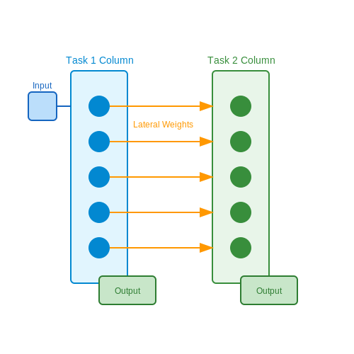
Progressive Neural Networks (PNNs) address catastrophic forgetting by introducing a modular architecture where each new task is learned by a separate column of neural networks, while preserving knowledge from previous tasks through lateral connections. This approach ensures that earlier representations remain intact while allowing new task-specific adaptations.
Architecture and Lateral Connections
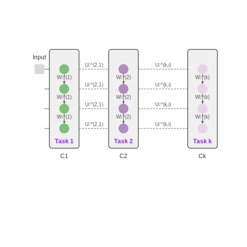
The core innovation of PNNs lies in their column-based design. For each new task k, a new neural network column Ck is instantiated. Lateral connections from all previous columns C1, C2, ..., Ck-1 feed into Ck, enabling the new column to leverage learned features without modifying the weights of prior columns. Mathematically, the input to layer l in column k is:
Here, Wl(k) denotes the weights of column k at layer l, while Ul(k,i) represents the lateral connection weights from column i to column k. The function f is a nonlinear activation, typically ReLU.
Training Dynamics
Training proceeds sequentially, freezing all parameters of previous columns when learning a new task. Only the weights of the new column Ck and its lateral connections are updated. This ensures:
- Stability: Existing knowledge is preserved since prior columns remain unchanged.
- Plasticity: New columns adapt to task-specific requirements without interference.
The loss function for task k is computed solely over the output of Ck, with gradients backpropagated only through the active column and its lateral connections.
Scalability and Efficiency
While PNNs eliminate forgetting, their parameter count grows linearly with the number of tasks. To mitigate this, techniques like weight pruning or shared lower-level representations can be applied. Recent variants, such as Condensed Progressive Neural Networks, compress lateral connections to reduce memory overhead while retaining performance.
Applications and Limitations
PNNs excel in scenarios requiring incremental learning, such as:
- Continual adaptation of robotics controllers to new environments.
- Sequential fine-tuning of medical diagnosis models for new diseases.
However, their rigid columnar structure can become inefficient for large-scale task sequences. Hybrid approaches combining PNNs with elastic weight consolidation or memory replay are active research areas.
3.3 Memory Replay Techniques
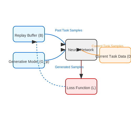
Memory replay techniques mitigate catastrophic forgetting by periodically retraining neural networks on stored or generated samples from previous tasks. These methods leverage the principle of interleaved learning, ensuring that the model retains knowledge of past distributions while adapting to new data.
Experience Replay
Experience replay stores a subset of past training samples in a fixed-size buffer, interleaving them with new task data during training. The loss function for a task t combines current and replayed samples:
where B is the replay buffer, and α balances current versus past task importance. The buffer is typically updated via reservoir sampling to maintain a representative distribution of historical data.
Generative Replay
Instead of storing raw data, generative replay trains a generative model (e.g., GAN or VAE) to synthesize pseudo-samples from previous tasks. The objective becomes:
Here, Gφ generates samples conditioned on labels y from historical label distributions. This avoids memory overhead but introduces approximation error from the generative model.
Optimization Strategies
Replay techniques often integrate with regularization-based approaches:
- Dark Experience Replay (DER): Augments replayed samples with logit-based distillation loss:
- Gradient Episodic Memory (GEM): Projects new task gradients to avoid interference with replay sample gradients, enforcing:
Architectural Extensions
Advanced variants include:
- Dual-Memory Systems: Separate short-term (current task) and long-term (replay) memory buffers with different sampling strategies.
- Dynamic Replay Scheduling: Adjusts replay frequency based on task similarity metrics or forgetting rates.
Empirical studies show replay methods achieve 15-30% higher accuracy than pure regularization on class-incremental benchmarks like Split-CIFAR100, at the cost of increased computational overhead proportional to the replay ratio.
3.4 Regularization-Based Approaches
Regularization-based methods mitigate catastrophic forgetting by constraining weight updates to preserve important parameters from previous tasks. These approaches modify the loss function to penalize deviations from learned representations, effectively balancing plasticity and stability.
Elastic Weight Consolidation (EWC)
EWC introduces a quadratic penalty term that anchors parameters to their optimal values from previous tasks, weighted by the Fisher information matrix. The loss function for task B becomes:
where θA,i* are the optimal parameters for task A, Fi is the Fisher information diagonal, and λ controls regularization strength. The Fisher matrix approximates parameter importance:
Synaptic Intelligence (SI)
SI computes online parameter importance during training via the loss gradient's path integral. The regularization term accumulates weight importance ωi over time:
where ξ is a decay factor. The loss then becomes:
Memory-Aware Synapses (MAS)
MAS estimates parameter importance through unsupervised sensitivity analysis. The importance Ωi is computed as:
where f(x;θ) is the network's output. This approach requires no task-specific labels during importance computation.
Comparative Analysis
These methods differ in computational overhead and theoretical guarantees:
- EWC provides Bayesian rigor but requires storing Fisher matrices
- SI offers online computation but depends on training trajectory
- MAS enables task-agnostic importance estimation
Recent variants like Online EWC and RWalk combine these approaches with importance sampling for improved scalability. Practical implementations often use diagonal approximations of the Fisher matrix to reduce memory requirements from O(n²) to O(n) for n parameters.
4. Measuring Forgetting in Continual Learning
4.1 Measuring Forgetting in Continual Learning
Quantifying catastrophic forgetting is essential for evaluating continual learning algorithms. Unlike static learning scenarios, where performance is measured on a fixed test set, continual learning requires dynamic metrics that capture knowledge retention across sequential tasks. Two primary approaches dominate the literature: task-specific forgetting measures and consolidated performance metrics.
Task-Specific Forgetting Metrics
Forgetting in a task-sequential setting is typically measured by comparing a model's performance before and after learning subsequent tasks. Let Rk,i denote the test accuracy of task k immediately after training on task i. The forgetting measure Fk for task k after learning n tasks is:
This captures the maximum drop in accuracy for task k due to interference from later tasks. The average forgetting across all K tasks is then computed as:
Consolidated Performance Metrics
Alternative approaches evaluate overall system performance rather than per-task forgetting. The backward transfer (BWT) metric quantifies how learning new tasks affects previous ones:
Negative BWT values indicate catastrophic forgetting, while positive values suggest beneficial knowledge transfer. Similarly, forward transfer (FWT) measures how prior learning improves performance on unseen tasks:
where Rk,0 represents performance on task k before any training.
Memory-Based Evaluation Protocols
When algorithms employ episodic memory buffers, additional metrics become relevant. The retained accuracy ratio (RAR) compares memory-augmented performance to the ideal single-task baseline:
where Rk,k* is the upper-bound accuracy when training solely on task k. The memory stability index tracks how well exemplars preserve original task information:
where M is the memory buffer, fn is the model after n tasks, and yx are the original labels.
Implementation Considerations
Practical evaluation requires careful experimental design:
- Task ordering control: Randomize task sequences to isolate algorithmic robustness from ordering effects
- Computational constraints: Track wall-clock time and memory overhead alongside accuracy metrics
- Statistical significance: Report mean and standard deviation across multiple random seeds
Recent benchmarks like Continual Learning Evaluation Protocol (CLEP) standardize these measurements across different algorithm classes, enabling fair comparison between regularization-based, architectural, and rehearsal-based approaches.
4.2 Standard Datasets and Tasks
Benchmark Datasets for Catastrophic Forgetting
Evaluating catastrophic forgetting requires datasets that simulate sequential learning scenarios. The most widely adopted benchmarks include:
- Split MNIST: The original MNIST dataset is divided into 5 sequential tasks, each containing two digit classes (e.g., Task 1: 0/1, Task 2: 2/3). This tests incremental class learning.
- Permuted MNIST: Each task applies a fixed random permutation to the pixel locations of MNIST images, creating distinct input distributions while maintaining the same output classes.
- Split CIFAR-10/100: Similar to Split MNIST but with more complex color images. CIFAR-100 is often split into 10 tasks of 10 classes each.
- Omniglot: Contains 1,623 character classes from 50 alphabets, often used for few-shot continual learning scenarios.
Standard Evaluation Protocols
Two key metrics quantify catastrophic forgetting:
where Ri,j is the test accuracy on task j after learning task i, and T is the total number of tasks.
Common Task Sequences
Researchers typically evaluate methods under three scenarios:
- Class-Incremental Learning: New classes appear in each task while old classes may reappear during testing.
- Domain-Incremental Learning: Input distribution changes (e.g., permuted pixels) while the underlying classes remain constant.
- Task-Incremental Learning: Each task has distinct input-output mappings, with task identity provided during testing.
Advanced Benchmarks
Recent work has introduced more challenging benchmarks:
- CORe50: 50 domestic objects captured in 11 sessions with varying backgrounds/illuminations.
- Stream-51: 51 object categories with temporal continuity constraints.
- OpenLORIS: Real-world robotics data with natural domain shifts.
The choice of dataset significantly impacts the observed forgetting behavior, with more complex tasks (e.g., CORe50) typically showing stronger catastrophic forgetting effects than simpler benchmarks like Split MNIST.
4.3 Comparative Analysis of Methods
Several approaches have been proposed to mitigate catastrophic forgetting in neural networks, each with distinct advantages and limitations. Below, we analyze the most prominent methods, comparing their computational overhead, scalability, and effectiveness across different task sequences.
Regularization-Based Methods
Methods like Elastic Weight Consolidation (EWC) and Synaptic Intelligence (SI) impose constraints on weight updates based on their importance to previous tasks. EWC approximates the Fisher information matrix to identify critical weights:
where Fi represents the Fisher information for parameter θi, and θi* denotes the optimal value for previous tasks. While computationally efficient, these methods struggle with long task sequences due to quadratic growth in constraints.
Architectural Methods
Progressive Neural Networks (PNNs) and PackNet avoid interference by expanding network capacity or partitioning weights. PNNs instantiate new columns for each task while maintaining lateral connections:
Though effective, architectural methods exhibit linear parameter growth with tasks, making them impractical for large-scale deployments. PackNet's iterative pruning-and-retraining achieves better parameter efficiency but requires task-specific masks during inference.
Replay-Based Methods
Experience Replay (ER) and Gradient Episodic Memory (GEM) store subsets of past data or gradients. GEM solves a constrained optimization problem:
While replay methods often achieve state-of-the-art performance, their memory footprint scales with task complexity. Recent hybrid approaches like DER++ combine replay with regularization, demonstrating superior trade-offs on benchmarks such as Split-CIFAR100.
Quantitative Comparison
| Method | Memory Overhead | Compute Overhead | Avg. Accuracy Drop |
|---|---|---|---|
| EWC | O(d) | Low | 22.4% |
| PNN | O(td) | High | 8.1% |
| GEM | O(tm) | Medium | 11.7% |
Key trade-offs emerge: regularization suits resource-constrained environments, while replay methods dominate when memory permits. Emerging directions include dynamic architectures (e.g., Sparse Neural Networks) and meta-learning approaches that optimize the plasticity-stability trade-off at a higher level.
5. Key Research Papers
5.1 Key Research Papers
- Understanding Catastrophic Forgetting and Remembering in Continual ... — the problem of catastrophic forgetting. But, unlike the prob-lem of catastrophic forgetting, which has a rich literature of research, catastrophic remembering has not been explored outside of minor discussions in early works (Sharkey & Sharkey,1995a;Lewandowsky & Li,1995;French,1991). In this work, we discuss CR from a probabilistic perspective
- REMIND Your Neural Network to Prevent Catastrophic Forgetting - Springer — Parisi et al. [] identify three main mechanisms for mitigating forgetting in neural networks, namely 1) replay of previous knowledge, 2) regularization mechanisms to constrain parameter updates, and 3) expanding the network as more data becomes available.Replay has been shown to be one of the most effective methods for mitigating catastrophic forgetting [4, 5, 13, 22, 27, 44, 45, 50, 59, 64, 77].
- Overcoming Catastrophic Forgetting in Heterogeneous Federated Learning — signing and implementing the methodology to mitigate catastrophic forget-ting, and conducting experiments to evaluate its effectiveness in heteroge-neous medical imaging datasets. Several collaborators contributed to this research. My co-author, Sana Ay-romlou, assisted with methodology design, carrying out experiments, and writing the paper.
- PDF Preventing Catastrophic Forgetting through Memory Networks in ... — of catastrophic forgetting have been developed for continual classification [13, 20,29,32,35,37,43,44], much fewer approaches have looked at more granular ... tion to the key through a similarity function, typically cosine similarity. The retrieved memory units are usually integrated within the multi-head attention
- PDF Catastophic Forgetting in Neural Networks - ox.no — is catastrophic forgetting in neural networks. The report starts by explaining the problem of catastrophic forgetting, and gives a broad survey of various solutions to the problem. Two of the most well known solutions to the problem are reproduced according to their original ex-perimental descriptions, and the results are found to be reproducible.
- PDF Overcoming Catastrophic Forgetting in Incremental Few-Shot ... - NeurIPS — proposed to optimize neural networks towards flat local minima. In this paper, we show that for incremental few-shot learning, finding flat minima in the base session and tuning the model within the flat region on new tasks can significantly mitigate catastrophic forgetting. 3 Severity of Catastrophic Forgetting in Incremental Few-Shot ...
- Understanding Catastrophic Forgetting and Remembering in Continual ... — Catastrophic forgetting in neural networks is a significant problem for continual learning. A majority of the current methods replay previous data during training, which violates the constraints ...
- PDF Solving the Catastrophic Forgetting Problem in Generalized Category ... — In summary, our key contributions are as follows: • We introduce a novel constraint named Local Entropy Regularization (LER), which is designed to mitigate the catastrophic forgetting problem of known classes by pre-serving the knowledge of known categories during learn-ing novel classes. • We propose a Dual-views Kullback-Leibler divergence
- Remembering for the right reasons: Explanations reduce catastrophic ... — performance and avoiding so-called catastrophic forgetting of previous experience3,4 when learning new skills. The goal is to develop algorithms that continually update or add parameters to accommodate an online stream of data over time. An active line of research in continual learning explores the effectiveness of using small memory budgets to ...
- Defying catastrophic forgetting via influence function — This paper adopts the concept of influence function to measure the importance of parameters so as to address catastrophic forgetting in deep neural networks (DNNs). The important notations are shown in Table F.14 of Appendix F. In the following section, this paper analyzes the regularization-based methods in terms of the estimator's asymptotic ...
5.2 Books and Review Articles
- REMIND Your Neural Network to Prevent Catastrophic Forgetting - Springer — Parisi et al. [] identify three main mechanisms for mitigating forgetting in neural networks, namely 1) replay of previous knowledge, 2) regularization mechanisms to constrain parameter updates, and 3) expanding the network as more data becomes available.Replay has been shown to be one of the most effective methods for mitigating catastrophic forgetting [4, 5, 13, 22, 27, 44, 45, 50, 59, 64, 77].
- Understanding Catastrophic Forgetting and Remembering in Continual ... — the problem of catastrophic forgetting. But, unlike the prob-lem of catastrophic forgetting, which has a rich literature of research, catastrophic remembering has not been explored outside of minor discussions in early works (Sharkey & Sharkey,1995a;Lewandowsky & Li,1995;French,1991). In this work, we discuss CR from a probabilistic perspective
- Handling Catastrophic Forgetting: Online Continual Learning for Next ... — This often prevents keeping all past data, but relying only on recent data introduces bias and causes catastrophic forgetting . Definition 8 (Catastrophic Forgetting ). Let there be a model at any point in time that has learned a sequence of \(\mathcal {T}\) learning tasks. When faced with the \((\mathcal {T} + 1)\) th task, the model tends to ...
- Remembering for the right reasons: Explanations reduce catastrophic ... — Incremental classifier and representation learning (iCaRL) 7 is a class-incremental learner that uses a nearest-exemplar algorithm for classification and prevents catastrophic forgetting by using an episodic memory. iTAML 6 is a task-agnostic meta-learning algorithm that uses a momentum-based strategy for meta-update and in addition to the ...
- PDF Catastophic Forgetting in Neural Networks - ox.no — is catastrophic forgetting in neural networks. The report starts by explaining the problem of catastrophic forgetting, and gives a broad survey of various solutions to the problem. Two of the most well known solutions to the problem are reproduced according to their original ex-perimental descriptions, and the results are found to be reproducible.
- Understanding Catastrophic Forgetting and Remembering in Continual ... — Catastrophic forgetting in neural networks is a significant problem for continual learning. A majority of the current methods replay previous data during training, which violates the constraints ...
- Overcoming Catastrophic Forgetting in Heterogeneous Federated Learning — 2.1 Catastrophic forgetting occurs when server weights are over-written during local training, causing a loss of previous knowl-edge. To investigate the effect of catastrophic forgetting dur-ing local training in FL, we conducted experiments on Blood-MNIST using the same experimental settings described in Sec. 3.2.
- Example forgetting and rehearsal in continual learning — Lifelong learning implies the capability to acquire new knowledge while preserving previously learned experiences. While we humans excel at this, artificial neural networks are prone to catastrophic forgetting [1] when they are trained on non-i.i.d. data belonging to different tasks, without access to the past ones. The field of continual learning (CL) [2] studies the training of models in ...
- Defying catastrophic forgetting via influence function — The digital world around us is continuously evolving [46].Each day, huge amounts of data such as images and videos are produced on social media, which generates new emerging learning tasks [44], [45].It is important for learning systems to adapt quickly to changing environments [47], [48], [50].For quick adaptation to occur, learning systems are required to memorize useful past experiences ...
- (PDF) Continual Learning: Tackling Catastrophic Forgetting in Deep ... — Nevertheless, because of the catastrophic forgetting phenomena, learning continually is a c halleng- ing discipline. The strategy consisting in saving everything to a void any forgetting is not ...
5.3 Online Resources and Tutorials
- Handling Catastrophic Forgetting: Online Continual Learning for Next ... — Handling Catastrophic Forgetting: Online Continual Learning 227. of previously learned information while integrating new insights, thereby maintaining a comprehensive understanding of the data distribution landscape. By leveraging task-specific and task-invariant features, continual learning helps to mitigate catastrophic forgetting.
- REMIND Your Neural Network to Prevent Catastrophic Forgetting - Springer — Parisi et al. [] identify three main mechanisms for mitigating forgetting in neural networks, namely 1) replay of previous knowledge, 2) regularization mechanisms to constrain parameter updates, and 3) expanding the network as more data becomes available.Replay has been shown to be one of the most effective methods for mitigating catastrophic forgetting [4, 5, 13, 22, 27, 44, 45, 50, 59, 64, 77].
- PSYC 5.3 (Learning and Memory: Forgetting and Amnesia) NF - Quizlet — Study with Quizlet and memorize flashcards containing terms like If you fail to _____ information into memory, you are not going to remember it later on, occur because we are distracted or are not paying attention to specific details, if we do not _____ memory and the neural representation of that memory is not reactivated over a long period of time, the memory representation may ...
- 5.3- forgetting and memory construction Flashcards - Quizlet — Study with Quizlet and memorize flashcards containing terms like Forgetting, retention, relearning and more.
- PDF REMIND Your Neural Network to Prevent Catastrophic Forgetting - ECVA — to data ordering schemes known to induce catastrophic forgetting. We demonstrate REMIND's generality by pioneering online learning for Vi-sual Question Answering (VQA)5. Keywords: Online Learning, Brain-inspired, Deep Learning 1 Introduction The mammalian brain engages in continuous online learning of new skills, ob-jects, threats, and ...
- Handling Catastrophic Forgetting: Online Continual Learning for Next ... — A significant challenge in online next activity prediction arises from adapting to new concepts following shifts in data distribution. While real-time model updates enable responsiveness to evolving trends and operational changes, they also introduce the risk of catastrophic forgetting . This phenomenon occurs when the prediction model ...
- Mitigating catastrophic forgetting in incremental learning - ResearchGate — The term catastrophic forgetting or catastrophic interference was first in troduced by McCloskey and Cohen[20]. Standard learning aims to learn jointly[21] or whenev er
- PDF Eindhoven University of Technology MASTER Online Process Prediction ... — primary focus on mitigating catastrophic forgetting. To assess the effectiveness of a method in mitigating catastrophic forgetting, we introduce new datasets and metrics. These datasets simulate scenarios with recurring concept drifts, allowing us to evaluate the method's performance when data from the same task reappears.
- AP Psychology - Unit 5.3 (Forgetting and False Memories) - Quizlet — the disruptive effect of new learning on the recall of old information (ex. Someone singing different lyrics to a song may cause you to have trouble remembering original lyrics)
- EXACFS - A CIL Method to Mitigate Catastrophic Forgetting — Figure 1: Schematic of the EXACFS Method.At incremental task t + 1, input comprises of samples from new classes and a few exemplars from classes of earlier tasks. Class labels are shown by colour coding. A shared but incrementally updated feature extractor extracts features. Features influencing class(es) decision are accordingly colour-coded, with the intensity of colour conveying the level ...