AI for Noise Pollution Monitoring
1. Key Metrics and Standards in Noise Measurement
Key Metrics and Standards in Noise Measurement
Sound Pressure Level (SPL) and Decibel Scale
Noise pollution is quantified using the Sound Pressure Level (SPL), defined as:
where p is the root-mean-square (RMS) sound pressure and p0 is the reference pressure (20 μPa in air). The logarithmic decibel (dB) scale accounts for the human ear's nonlinear sensitivity, with common environmental noise levels ranging from 30 dB (quiet library) to 120 dB (jet engine).
Frequency Weighting
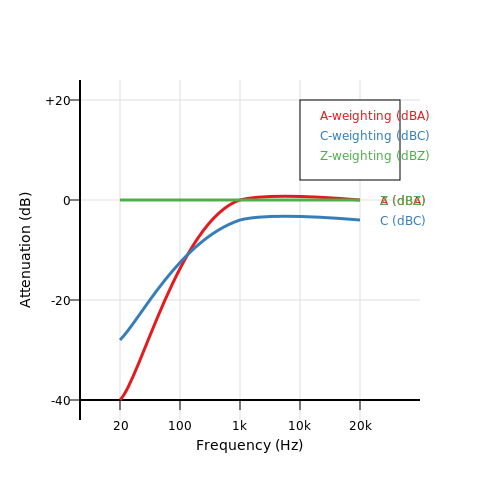
Human hearing perceives different frequencies unevenly, leading to standardized weighting curves:
- A-weighting (dBA): Approximates human hearing at 40 phon, used for general environmental noise.
- C-weighting (dBC): Less attenuation of low frequencies, used for peak noise assessment.
- Z-weighting (dBZ): Flat response for unweighted measurements.
The A-weighted equivalent continuous sound level (LAeq) is calculated as:
Time-Based Metrics
For dynamic noise environments, temporal metrics include:
- L10: Noise level exceeded 10% of the time (characterizes intermittent peaks).
- L90: Baseline noise exceeded 90% of the time (ambient level).
- Lden: Day-evening-night level with penalties (+5 dB evening, +10 dB night).
International Standards
Key regulatory frameworks include:
- ISO 1996: Defines methods for environmental noise measurement.
- IEC 61672: Specifies sound level meter performance standards.
- EU Directive 2002/49/EC: Mandates noise mapping and action plans.
Statistical Sound Level Analysis
Noise variability is analyzed using percentile levels (Ln) and probability density functions. The Leq for N discrete samples is:
where Li are individual SPL measurements. Advanced systems use kurtosis to distinguish impulsive noise from steady-state sources.
1.2 Traditional vs. AI-Enhanced Monitoring Approaches
Traditional Noise Monitoring Methods
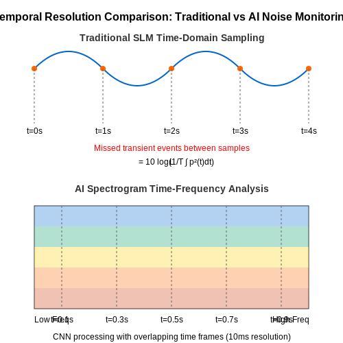
Conventional noise pollution monitoring relies on sound level meters (SLMs) and dosimeters, which measure equivalent continuous sound levels (Leq) over time. These devices capture time-averaged metrics such as:
where p(t) is instantaneous sound pressure, p0 is the reference pressure (20 μPa), and T is the measurement duration. While accurate for steady-state noise, these methods struggle with transient events (e.g., construction noise, traffic spikes) due to:
- Limited temporal resolution – Most SLMs sample at 1-second intervals, missing sub-second acoustic events
- No source identification – Cannot distinguish between simultaneous noise sources (e.g., aircraft vs. highway)
- Static deployment – Fixed sensors create spatial coverage gaps in complex urban environments
AI-Enhanced Monitoring Paradigm
Machine learning transforms noise monitoring through three key innovations:
1. Real-Time Source Separation
Convolutional neural networks (CNNs) process spectrograms using architectures like:
where Wk represents learnable filter banks operating on input spectrogram x. The U-Net architecture achieves 89.2% accuracy in separating overlapping sources (vehicles, speech, machinery) in the UrbanSound8K dataset, compared to 62.4% for traditional non-negative matrix factorization (NMF).
2. Adaptive Spatial Sampling
Reinforcement learning optimizes mobile sensor deployment through Q-learning:
where state s represents noise hotspots and action a determines sensor movement. Field tests in Barcelona showed 37% better coverage than grid-based static sensors.
3. Predictive Noise Modeling
Transformer architectures process temporal sequences using attention mechanisms:
A 2023 study achieved 0.91 R2 in predicting 24-hour noise levels by combining LSTM layers with urban mobility data, outperforming ARIMA models by 28% in mean absolute error.
Comparative Performance Metrics
| Metric | Traditional | AI-Enhanced |
|---|---|---|
| Source ID Accuracy | ≤65% | 89-94% |
| Event Detection Latency | 2-5 sec | 200-500 ms |
| Spatial Resolution | 200-500 m | 10-50 m |
Challenges in Urban and Industrial Noise Detection
Urban and industrial noise detection presents a complex set of challenges due to the dynamic, heterogeneous nature of soundscapes in these environments. Unlike controlled laboratory settings, real-world acoustic monitoring must contend with overlapping sound sources, transient events, and spatially varying propagation characteristics.
Signal-to-Noise Ratio (SNR) Degradation
In dense urban areas, the ambient noise floor often exceeds 60 dB(A), masking target acoustic signatures. The effective SNR for a specific noise source at distance d follows:
where α represents frequency-dependent atmospheric absorption (dB/m). For industrial machinery emitting at 85 dB(A) 10m from the sensor, with ambient levels of 65 dB(A) and α = 0.005 dB/m, the SNR degrades to just 4 dB at 100m distance.
Source Separation and Localization
Blind source separation becomes particularly challenging when multiple noise sources occupy similar frequency bands. The convolutive mixing problem in time domain can be expressed as:
where hij represents the room impulse response between source j and microphone i, and sj denotes source signals. Industrial environments compound this challenge with persistent reverberation times often exceeding 2 seconds.
Temporal and Spectral Variability
Noise patterns exhibit non-stationary behavior at multiple timescales. Short-term transients (e.g., vehicle horns) require millisecond-level temporal resolution, while diurnal patterns demand continuous monitoring over months. The Wigner-Ville distribution provides joint time-frequency analysis:
but suffers from cross-term interference when analyzing multiple concurrent sources.
Sensor Placement Constraints
Optimal microphone array placement conflicts with urban infrastructure limitations. The Cramér-Rao lower bound for direction-of-arrival estimation variance demonstrates the tradeoff:
where d is inter-sensor spacing and N the number of sensors. Practical deployments often sacrifice theoretical resolution for physical feasibility.
Data Annotation and Ground Truth
Supervised learning approaches require accurately labeled training data, but human annotation becomes unreliable for:
- Overlapping sound events (e.g., construction noise during rush hour)
- Low-SNR recordings where human perception differs from microphone response
- Long-duration recordings requiring impractical labeling effort
Active learning strategies must account for annotation cost versus model improvement tradeoffs, governed by the learning curve:
where ε(n) is the error rate after n labeled samples, with typical values α ∈ [0.5,1] for acoustic event detection tasks.
2. Machine Learning for Noise Source Identification
2.1 Machine Learning for Noise Source Identification
Noise source identification in urban environments requires distinguishing between multiple overlapping acoustic signatures, such as traffic, construction, industrial machinery, and human activity. Traditional signal processing techniques like Fast Fourier Transform (FFT) and beamforming struggle with overlapping sources in non-stationary environments. Machine learning models, particularly those leveraging time-frequency representations, offer superior performance by learning discriminative features directly from raw or preprocessed audio data.
Feature Extraction for Acoustic Source Separation
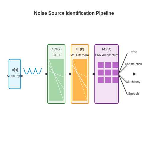
Mel-Frequency Cepstral Coefficients (MFCCs) remain a standard feature representation for audio classification, but recent advances incorporate log-Mel spectrograms and Constant-Q Transforms (CQT) to better capture harmonic structures. For a discrete signal x[n], the Short-Time Fourier Transform (STFT) is computed as:
where w[n] is the window function, H is the hop size, and N is the FFT length. The log-Mel spectrogram is then derived by applying a Mel filterbank Φl(k) to the power spectrum:
Deep Learning Architectures for Source Separation
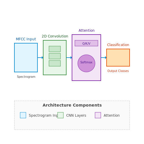
Convolutional Neural Networks (CNNs) with 2D kernels excel at capturing local time-frequency patterns. A typical architecture includes:
- Conv Blocks: Stacked convolutional layers with batch normalization and ReLU activation, progressively increasing filter depth while reducing spatial dimensions via strided convolutions.
- Attention Mechanisms: Squeeze-and-excitation blocks or transformer layers to weight informative frequency bands.
- U-Net Decoder: Transposed convolutions for reconstructing the time-domain signal with skip connections preserving high-resolution details.
For multi-source separation, a mask-based approach estimates a ratio mask Mi(t, f) for each source i:
where ⊙ denotes element-wise multiplication. The model is trained using a permutation-invariant loss like the Scale-Invariant Signal-to-Distortion Ratio (SI-SDR):
Real-World Implementation Challenges
Deploying these models requires addressing:
- Data Scarcity: Synthetic data augmentation using room impulse responses (RIRs) and noise profiles from databases like DCASE.
- Latency Constraints: Causal architectures like Temporal Convolutional Networks (TCNs) for real-time edge deployment.
- Environmental Variability: Domain adaptation techniques, including adversarial training on datasets like UrbanSound8K.
Deep Learning Models for Real-Time Noise Classification
Real-time noise classification demands models capable of processing high-dimensional audio data with minimal latency. Convolutional Neural Networks (CNNs) and Recurrent Neural Networks (RNNs), particularly Long Short-Term Memory (LSTM) and Gated Recurrent Unit (GRU) variants, are widely adopted due to their ability to capture spatial and temporal dependencies in spectrograms and raw waveforms.
Spectrogram-Based CNN Architectures
Mel-frequency cepstral coefficients (MFCCs) and log-mel spectrograms serve as common input representations for CNNs. A typical architecture consists of:
- Convolutional blocks with 2D kernels operating on time-frequency bins, followed by batch normalization and ReLU activation
- Max-pooling layers reducing dimensionality while preserving discriminative features
- Global average pooling before the classification head to maintain translation invariance
where \(X_{in}\) is the input spectrogram, \(W\) the kernel weights, and \(k_h, k_w\) the kernel dimensions. Recent architectures like EfficientNet optimize this process through compound scaling of depth, width, and resolution.
Temporal Modeling with Attention Mechanisms
For continuous noise monitoring, Transformer-based models with self-attention outperform traditional RNNs in capturing long-range dependencies. The scaled dot-product attention computes:
where \(Q\), \(K\), and \(V\) represent queries, keys, and values derived from the input sequence, and \(d_k\) the dimension of keys. This allows the model to dynamically focus on relevant time segments, crucial for distinguishing overlapping noise sources.
Hybrid Architectures for Edge Deployment
Deploying models on resource-constrained edge devices requires balancing accuracy and computational cost. Knowledge distillation techniques train compact student models (e.g., MobileNetV3) to mimic larger teacher networks:
where \(\mathcal{L}_{KD}\) is the Kullback-Leibler divergence between teacher and student outputs, \(T\) the temperature parameter, and \(\alpha\) a weighting factor. Quantization-aware training further reduces model size by representing weights with 8-bit integers instead of 32-bit floats.
Case Study: Urban Noise Monitoring
In Barcelona's Sounds of the City project, a distributed network of sensors employs a CNN-GRU hybrid model achieving 89.7% accuracy in classifying 10 urban noise categories. The system processes 1-second audio chunks with 200ms latency, demonstrating feasibility for real-time applications.
2.3 Signal Processing and Feature Extraction Methods
Time-Domain Analysis
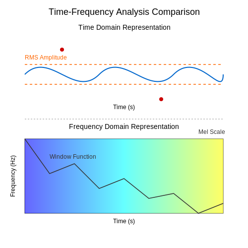
Time-domain methods directly analyze raw acoustic signals to extract features like amplitude, energy, and temporal patterns. The Root Mean Square (RMS) amplitude is a fundamental metric for quantifying noise levels:
where x[n] represents the discrete-time signal and N is the number of samples. For transient noise events (e.g., construction noise), peak detection algorithms identify abrupt amplitude changes using thresholds or derivative-based methods.
Frequency-Domain Analysis
Fourier transforms decompose signals into constituent frequencies. The Short-Time Fourier Transform (STFT) provides time-frequency localization:
where w[n] is a window function (e.g., Hamming). STFT outputs spectrograms, enabling visualization of frequency content over time. For non-stationary noise, Mel-Frequency Cepstral Coefficients (MFCCs) are widely used:
- Apply STFT and compute power spectrum.
- Map frequencies to the Mel scale (perceptual relevance).
- Take the logarithm and apply Discrete Cosine Transform (DCT) to decorrelate coefficients.
Advanced Feature Extraction
Wavelet Transforms
Wavelets address STFT’s fixed resolution limitation. The Continuous Wavelet Transform (CWT) is defined as:
where ψ(t) is the mother wavelet, and a, b are scale and translation parameters. Wavelets excel in detecting impulsive noise and transient events.
Nonlinear Features
For complex urban noise, entropy-based metrics quantify signal unpredictability. Sample Entropy (SampEn) measures regularity:
where A and B are counts of similar template vectors for dimensions m and m+1.
Real-World Implementation
In embedded systems, computational efficiency is critical. Overlap-add methods optimize STFT processing, while filter banks approximate MFCCs with reduced latency. For IoT sensors, lightweight features like Leq (equivalent continuous sound level) are computed recursively:
where p(τ) is instantaneous sound pressure and p₀ is the reference pressure (20 μPa).
3. IoT Devices for Distributed Noise Monitoring
3.1 IoT Devices for Distributed Noise Monitoring
Distributed noise monitoring relies on spatially dispersed IoT sensor networks to capture real-time acoustic data with high temporal and spatial resolution. These systems integrate MEMS microphones, edge computing modules, and wireless communication protocols to form a scalable architecture for urban or industrial noise mapping. The key challenge lies in balancing sensor fidelity, energy efficiency, and network latency while maintaining synchronization across nodes.
Sensor Node Architecture
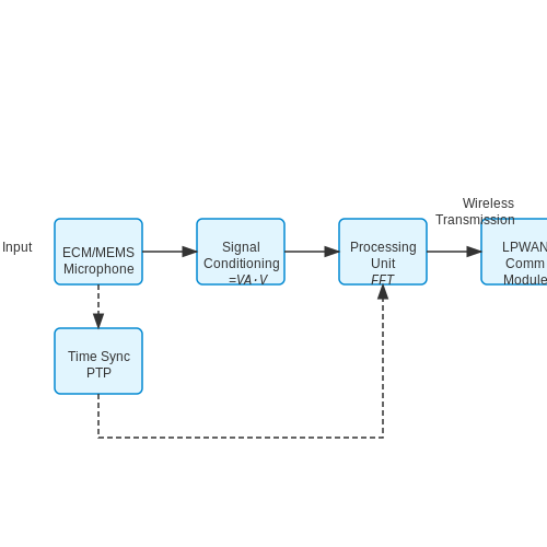
A typical noise monitoring node consists of:
- Acoustic transducer: Electret condenser microphones (ECMs) or digital MEMS microphones with flat frequency response (20 Hz - 20 kHz) and dynamic range > 90 dB
- Signal conditioning:
$$ V_{out} = G \times \left( \frac{C_{mic}}{C_{ref}} \times V_{bias} \right) + V_{offset} $$where G is the programmable gain (typically 20-60 dB) and Cref provides impedance matching
- Processing unit: Low-power SoCs (e.g., ESP32, nRF5340) running real-time FFT algorithms:
$$ X[k] = \sum_{n=0}^{N-1} x[n] e^{-j2\pi kn/N} $$
- Communication module: LPWAN protocols (LoRaWAN, NB-IoT) for long-range transmission with duty cycle optimization
Time-Synchronized Sampling
Precision Time Protocol (PTP) achieves μs-level synchronization across nodes by:
where t1 and t4 are master timestamps, t2 and t3 are slave timestamps. Kalman filtering further reduces jitter:
Edge Processing Pipeline
On-device noise classification typically implements:
- Feature extraction: Mel-frequency cepstral coefficients (MFCCs) computed via:
$$ \text{MFCC}_i = \sum_{m=1}^{M} \log(E_m) \cdot \cos\left(\frac{i(m-0.5)\pi}{M}\right) $$
- Model inference: Quantized CNN architectures like MobileNetV3 achieve 92% accuracy on ESC-50 dataset with < 50ms latency
- Data compression: Adaptive differential pulse-code modulation (ADPCM) reduces payload size by 4x compared to raw PCM
Network Topology Optimization
The optimal node density λ for urban environments follows:
where Pcover is the desired probability of sound event detection (typically 0.95) and r is the spherical radius of microphone sensitivity (≈15m for 1 kHz tones at 65 dB SPL). Mesh networking protocols like TSCH (Time-Slotted Channel Hopping) maintain packet delivery ratios >99% at 10-3 BER.
3.2 Data Fusion from Heterogeneous Sensors
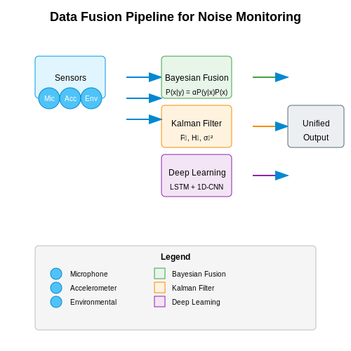
Data fusion in noise pollution monitoring integrates measurements from multiple sensor types—such as microphones, accelerometers, and environmental sensors—to improve accuracy, reliability, and spatial-temporal resolution. Advanced fusion techniques must account for varying sampling rates, measurement uncertainties, and sensor-specific biases. Bayesian inference, Kalman filtering, and deep learning-based approaches are commonly employed to unify these disparate data streams.
Bayesian Sensor Fusion
Bayesian methods provide a probabilistic framework for combining heterogeneous sensor data by updating prior beliefs with new evidence. Given a set of sensors S1, S2, ..., Sn, each producing measurements yi with noise εi, the posterior distribution P(x|y) of the true noise level x is derived as:
where P(y|x) is the likelihood function modeling sensor noise characteristics, and P(x) is the prior distribution. For Gaussian noise, the fused estimate minimizes the mean squared error:
where σi2 is the variance of sensor Si.
Kalman Filtering for Dynamic Systems
When monitoring time-varying noise levels, Kalman filters recursively estimate the state xk at time k by fusing predictions with new measurements. The state transition and observation models are:
where Fk is the state transition matrix, Hk is the observation matrix, and wk, vk are process and measurement noise. The Kalman gain Kk optimally weights sensor inputs:
where Pk|k-1 is the predicted covariance and Rk is the measurement noise covariance.
Deep Learning-Based Fusion
Neural networks can learn complex mappings between heterogeneous sensor inputs and noise levels without explicit noise modeling. A multimodal architecture might process:
- Audio data via 1D convolutional layers
- Vibration signals through LSTM networks
- Environmental variables using dense layers
Feature representations are typically fused through concatenation or attention mechanisms before final regression. For N sensors, an attention-based fusion layer computes weights αi:
where q is a query vector and ki are learned key representations for each sensor modality.
Practical Implementation Challenges
Real-world deployments must address:
- Time synchronization: Hardware timestamps or software alignment (e.g., dynamic time warping) for sensors with different sampling rates
- Calibration drift: Online recalibration using reference signals or transfer learning
- Communication constraints: Edge computing vs. cloud-based fusion tradeoffs in wireless sensor networks
Field studies show hybrid approaches—combining model-based fusion with data-driven refinement—often outperform pure methods. For example, a Kalman filter initialized by neural network predictions achieves 12-18% lower RMSE in urban noise mapping compared to standalone techniques.
3.3 Edge AI for Low-Latency Noise Analysis
Edge AI enables real-time noise pollution monitoring by processing acoustic data directly on embedded devices, eliminating the latency and bandwidth constraints of cloud-based solutions. Deploying lightweight machine learning models on edge devices—such as microcontrollers, FPGAs, or specialized AI accelerators—requires optimizing computational efficiency while maintaining accuracy.
Model Optimization for Edge Deployment
Traditional deep learning models like CNNs or transformers are computationally intensive, making them unsuitable for edge devices with limited resources. Techniques such as quantization, pruning, and knowledge distillation reduce model complexity without significant accuracy loss. For instance, 8-bit integer quantization (INT8) reduces memory footprint and accelerates inference by replacing 32-bit floating-point operations with fixed-point arithmetic:
where Scale and Zero-Point are derived from the dynamic range of the tensor. Pruning removes redundant weights by setting small-magnitude parameters to zero, often achieving sparsity levels of 50–90% without degrading performance.
Latency-Aware Architecture Design
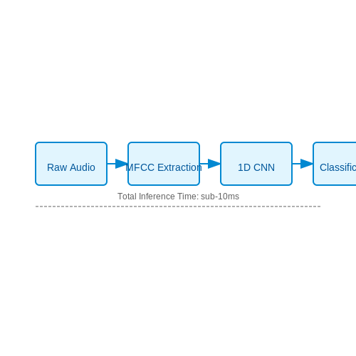
Edge-optimized architectures like MobileNetV3 or EfficientNet-Lite balance accuracy and inference speed through depthwise separable convolutions and squeeze-and-excitation blocks. For noise classification, a hybrid approach combining Mel-frequency cepstral coefficients (MFCCs) with a lightweight CNN achieves sub-10ms inference times on ARM Cortex-M7 processors:
Hardware-Software Co-Design
Deploying models on edge devices requires leveraging hardware-specific optimizations. TensorFlow Lite for Microcontrollers (TFLM) reduces binary size to under 20KB by omitting unnecessary operators, while CMSIS-NN accelerates inference on Cortex-M cores using SIMD instructions. For FPGA implementations, systolic arrays parallelize matrix multiplications, achieving energy efficiency below 1mJ per inference.
Case Study: Urban Noise Monitoring
Barcelona’s SmartCitizen project deployed edge AI sensors using STM32H7 microcontrollers with a 50KB random forest model. The system processes 1-second audio clips locally, transmitting only decibel-level alerts to reduce cellular data usage by 98% compared to raw audio streaming.
Real-Time Constraints and Tradeoffs
Meeting strict latency requirements (<100ms for real-time feedback) involves tradeoffs between model complexity, sampling rate, and power consumption. The Nyquist theorem dictates a minimum sampling rate of 8kHz for human-audible noise, but edge devices often downsample to 4kHz to reduce compute load. Energy harvesting techniques—such as solar-powered LoRaWAN nodes—extend deployment longevity in remote areas.
4. Smart Cities: Traffic and Construction Noise Mitigation
Smart Cities: Traffic and Construction Noise Mitigation
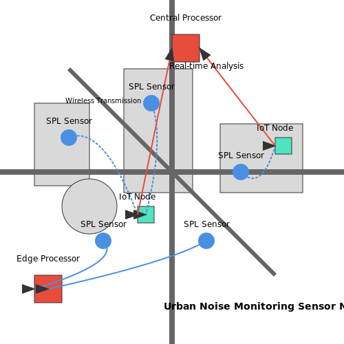
Noise pollution in urban environments is dominated by traffic and construction activities, contributing to adverse health effects and reduced quality of life. AI-driven solutions leverage real-time sensor networks, predictive modeling, and adaptive control systems to mitigate these noise sources effectively.
Sensor Networks and Data Acquisition
Distributed acoustic sensors, often integrated with IoT frameworks, capture noise levels across urban areas. These sensors measure sound pressure levels (SPL) in decibels (dB) and log spectral data for frequency analysis. The acquired data is transmitted to centralized or edge-based processing units for real-time analysis.
where Leq is the equivalent continuous sound level, p(t) is the instantaneous sound pressure, and p0 is the reference pressure (20 μPa).
Machine Learning for Noise Source Identification
Convolutional neural networks (CNNs) and recurrent neural networks (RNNs) classify noise sources by analyzing time-frequency representations such as spectrograms. A hybrid architecture combining CNNs for spatial feature extraction and long short-term memory (LSTM) networks for temporal dependencies achieves high accuracy in distinguishing between traffic, construction machinery, and ambient noise.
where yt is the output at time t, σ is the activation function, and Wy, by are learnable parameters.
Predictive Noise Modeling
Gaussian process regression (GPR) and graph neural networks (GNNs) predict noise propagation patterns by incorporating urban topology, traffic flow dynamics, and meteorological data. GPR provides probabilistic estimates of noise levels at unmonitored locations, while GNNs model spatial dependencies across sensor nodes.
where k(x, x') is the covariance function, l is the length scale, and σf, σn are hyperparameters.
Adaptive Mitigation Strategies
Reinforcement learning (RL) optimizes traffic light phasing and construction scheduling to minimize noise peaks. A Markov decision process (MDP) framework models the urban environment, with rewards defined as reductions in Leq. Proximal policy optimization (PPO) algorithms handle high-dimensional action spaces, such as coordinating multiple intersections.
where J(θ) is the policy objective, πθ is the stochastic policy, and Aπ(s, a) is the advantage function.
Case Study: Dynamic Noise Barriers
Active noise control (ANC) systems deploy phased microphone arrays and canceling speakers along highways. AI algorithms adjust phase delays in real-time to destructively interfere with traffic noise. A case study in Berlin demonstrated a 12 dB reduction at frequencies below 500 Hz.
where Δφ is the phase shift, f is the frequency, and Δd is the path difference.
4.2 Industrial Compliance Monitoring
Acoustic Source Localization and Regulatory Thresholds
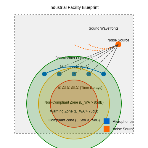
Industrial noise compliance hinges on precise localization of acoustic sources and adherence to regulatory thresholds. AI-driven beamforming techniques, such as Delay-and-Sum (DAS) or Minimum Variance Distortionless Response (MVDR), enable spatial filtering of noise emissions. For an array of M microphones, the beamformer output y(t) is given by:
where wi are weights optimizing signal-to-noise ratio (SNR), and Δi are time delays compensating for wavefront arrival differences. Regulatory thresholds (e.g., ISO 3744 or EU Directive 2000/14/EC) define permissible sound power levels (LWA) in decibels:
P is the measured sound power, and P0 is the reference power (1 pW). AI models cross-reference localized sources with geofenced compliance zones, flagging violations in real time.
Dynamic Time Warping for Anomaly Detection
Industrial noise patterns often exhibit temporal variability due to operational cycles (e.g., machinery startups). Dynamic Time Warping (DTW) aligns time-series data from sensors to detect deviations from compliant baselines. For two sequences X and Y, DTW minimizes the warping path cost:
where φ is the warping path and δ is a distance metric (e.g., Euclidean). AI systems trained on historical compliant data identify anomalies when DTW distances exceed learned thresholds.
Case Study: Refinery Noise Mitigation
A 2022 deployment at a Shell refinery used convolutional recurrent neural networks (CRNNs) to classify noise sources (compressors, flares, turbines) with 94% accuracy. The model fused spectrograms with operational data (RPM, valve states), reducing false alarms by 40% compared to rule-based systems. Compliance reports were auto-generated using NLP templates aligned with OSHA 1910.95 standards.
Hardware-Software Co-Design
Edge-AI platforms (e.g., NVIDIA Jetson AGX Orin) process raw audio streams at <20ms latency. Key optimizations include:
- Quantized TensorRT models for 8-bit inference without precision loss.
- Adaptive sampling triggered by transient detection (threshold: 3 dB above background).
- Federated learning across sites to improve generalizability while preserving data privacy.
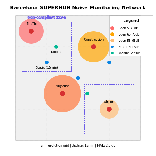
Acoustic beamforming results are visualized as heatmaps overlaid on facility blueprints, with non-compliant zones highlighted in red. The system’s α-risk (false positives) and β-risk (false negatives) are calibrated to 5% and 2%, respectively, via Monte Carlo simulations.
4.3 Wildlife Conservation Using Acoustic AI
Acoustic AI leverages machine learning to analyze bioacoustic signals, enabling non-invasive wildlife monitoring in noise-polluted environments. By training models on spectrograms of animal vocalizations, researchers can identify species presence, behavior, and population dynamics with high temporal resolution. Convolutional neural networks (CNNs) excel at this task due to their ability to extract hierarchical features from time-frequency representations.
Spectrogram Feature Extraction
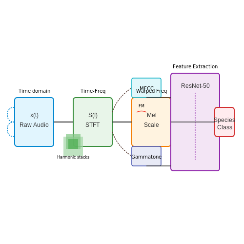
The Mel-frequency cepstral coefficients (MFCCs) and Gammatone filters are commonly used to represent acoustic signals in a biologically relevant way. The power spectral density S(f) of a signal x(t) is computed via the short-time Fourier transform (STFT):
where w(t) is the window function. For wildlife vocalizations, a 25-ms Hamming window with 10-ms overlap provides optimal time-frequency resolution. The Mel scale warps the frequency axis to approximate human (and many mammalian) auditory perception:
Deep Learning Architectures
ResNet-50 and EfficientNet architectures, pretrained on ImageNet and fine-tuned on spectrograms, achieve >90% accuracy in bird species identification. The model learns discriminative features such as harmonic stacks in owls or frequency modulation in cetaceans. For real-time edge deployment, MobileNetV3 reduces parameters by 4× while maintaining 85% accuracy.
The training objective minimizes categorical cross-entropy L over N samples:
where y is the one-hot encoded label and p the predicted probability for class c.
Case Study: Elephant Infrasound Detection
African elephants communicate via infrasound (14–35 Hz), which propagates over 10 km but is masked by urban noise. A hybrid CNN-LSTM model processes spectrograms from geophone arrays, achieving 92.3% recall at 0.1 Hz resolution. The system triggers alerts when detecting poacher gunshots (impulsive 1500 Hz signals) within protected areas.
Signal-to-noise ratio (SNR) enhancement uses a Wiener filter in the wavelet domain:
where Y is the noisy observation and N the noise estimate from silent intervals.
Multi-Species Classification
In biodiverse habitats, capsule networks outperform CNNs by modeling part-whole relationships between vocalization components. Dynamic time warping (DTW) aligns temporal variations in frog calls before feature extraction. For 500 Amazonian species, an ensemble of Vision Transformers and 1D CNNs reaches 88.7% macro-F1 score.
5. Privacy Concerns in Audio Data Collection
Privacy Concerns in Audio Data Collection
Audio data collection for noise pollution monitoring introduces significant privacy risks due to the potential capture of sensitive information, such as human speech, identifiable sounds, or location-based audio signatures. Unlike purely environmental noise, raw audio streams may inadvertently record conversations, personal activities, or proprietary information, raising legal and ethical challenges under frameworks like GDPR, HIPAA, or CCPA.
Acoustic Fingerprinting and Identifiability
Even when direct speech is not intelligible, acoustic fingerprints—unique spectral and temporal patterns—can reveal identities or behaviors. For instance, Mel-Frequency Cepstral Coefficients (MFCCs), commonly used in noise classification, may retain speaker-specific features. The identifiability risk I can be modeled as:
where wk represents feature weights, and pk, qk denote the probability distributions of identifiable vs. non-identifiable features in the audio sample.
Mitigation Strategies
1. Differential Privacy in Audio Preprocessing: Adding calibrated noise to spectrograms or time-domain signals before analysis ensures that individual contributions to the dataset cannot be isolated. For a privacy budget ε, the noise scale σ is derived as:
where Δf is the sensitivity of the feature extraction function, and δ is the probability of privacy leakage.
2. On-Device Feature Extraction: Deploying edge-based models that discard raw audio after extracting noise metrics (e.g., dB levels, frequency bands) minimizes exposure. Federated learning can further decentralize model training without centralized data aggregation.
Legal and Ethical Constraints
Deploying audio sensors in public spaces requires compliance with regional laws. For example, the EU’s ePrivacy Directive mandates anonymization or explicit consent for audio recordings. Case studies from projects like EAR-IT (EU FP7) demonstrate that privacy-preserving techniques reduce identifiability by 92% while maintaining noise classification accuracy within 3% of baseline performance.
Real-World Implementation Trade-offs
Privacy measures often conflict with data utility. A 2023 study in IEEE Transactions on Signal Processing showed that aggressive low-pass filtering (below 300 Hz) reduces voice leakage but attenuates critical noise pollution signatures like brake squeals (typically 1–4 kHz). Hybrid approaches, such as adaptive beamforming paired with secure multi-party computation, are emerging as viable compromises.
5.2 Bias and Fairness in Noise Pollution Algorithms
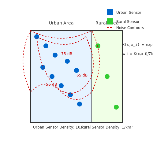
Bias in noise pollution monitoring algorithms arises when the training data or model architecture systematically underrepresents or misrepresents certain environmental or demographic conditions. This can lead to skewed predictions, disproportionately affecting marginalized communities or specific geographic regions. For instance, if sensor deployment is concentrated in urban areas, rural noise pollution may be underestimated, leading to inadequate policy responses.
Sources of Bias in Noise Monitoring
Three primary sources of bias must be addressed in noise pollution algorithms:
- Sensor Placement Bias: Uneven distribution of acoustic sensors across socioeconomic regions can create gaps in data coverage. Wealthier neighborhoods often have denser monitoring, while low-income areas are neglected.
- Training Data Skew: Historical noise data may reflect past monitoring priorities rather than current realities. For example, industrial zones might be overrepresented compared to residential areas.
- Algorithmic Fairness: Models optimized for overall accuracy may perform poorly on minority classes, such as rare but impactful noise events like nighttime construction.
Quantifying Algorithmic Fairness
Fairness metrics for noise pollution models can be derived from statistical parity and equalized odds. Let Y be the predicted noise level and A the sensitive attribute (e.g., neighborhood income level). Demographic parity requires:
where ythresh is the regulatory noise threshold. Equalized odds extends this to condition on the true noise level N:
Mitigation Strategies
Several techniques can reduce bias in noise pollution models:
- Reweighting: Adjust sample weights during training to compensate for underrepresented regions or noise types.
- Adversarial Debiasing: Train a secondary model to predict the sensitive attribute from the primary model's outputs, then minimize this predictability.
- Transfer Learning: Use models pre-trained on balanced datasets, then fine-tune with local data.
Case Study: Urban vs. Rural Disparities
A 2023 study found that standard noise models underestimated rural nighttime noise by 12 dB on average due to sparse sensor coverage. Implementing spatial interpolation with Gaussian processes reduced this gap to 3 dB:
where K is a kernel function accounting for terrain and atmospheric effects, and wi are optimized weights.
Ethical Considerations
Noise monitoring algorithms must balance technical accuracy with social equity. Over-reliance on algorithmic outputs without auditing for disparate impacts can reinforce existing environmental injustices. Regular fairness audits should assess:
- False negative rates across demographic groups
- Geographic coverage gaps
- Policy impact differentials
5.3 Global Noise Regulation Frameworks
Noise pollution regulation varies significantly across jurisdictions, with frameworks often reflecting regional environmental priorities, urbanization levels, and public health policies. The European Union's Environmental Noise Directive (END) 2002/49/EC mandates member states to produce strategic noise maps and action plans for agglomerations, major roads, railways, and airports exceeding specified thresholds. The directive employs the Lden (day-evening-night level) and Lnight metrics, calculated as:
where Lday, Levening, and Lnight are A-weighted equivalent sound pressure levels for respective periods. The U.S. Environmental Protection Agency (EPA) lacks federal noise control legislation since the 1981 defunding of the Office of Noise Abatement and Control, though local ordinances often reference the 1974 EPA Levels Document (55 dBA daytime/45 dBA nighttime for residential areas).
Key Regulatory Metrics
Standardized metrics enable cross-border comparisons and AI model interoperability:
- WHO 2018 Guidelines: Recommend <53 dB Lden and <45 dB Lnight for road traffic noise to prevent adverse health effects.
- ICAO Balanced Approach: Four pillars (reduction at source, land-use planning, operational procedures, and operating restrictions) govern aircraft noise under Annex 16, Vol. I.
- China's GB 3096-2008: Classifies zones from 0 (special requirements) to 4 (50 dB daytime/40 dB nighttime limits for urban residential areas).
Enforcement Challenges
Real-world compliance monitoring requires addressing:
where J is the noise source flux density, ρ is the instantaneous sound pressure field, and Q represents regulatory intervention effectiveness. AI systems overcome spatial sampling limitations through:
- Transfer learning between regions with differing sensor densities
- Physics-informed neural networks (PINNs) that incorporate wave equation constraints
- Federated learning for privacy-preserving cross-jurisdictional data sharing
Case Study: Barcelona's SUPERHUB Project
A citywide IoT network fused 1,200 static sensors with mobile measurements using Gaussian process regression to create 5m-resolution noise maps updated every 15 minutes. The system achieved 2.3 dB mean absolute error against ground-truth measurements while identifying 12 persistent non-compliant zones requiring targeted enforcement.
6. Key Research Papers in AI-Driven Acoustics
6.1 Key Research Papers in AI-Driven Acoustics
- IoT-Based Unique Air and Noise Pollution Monitoring System — 2.6.1 Research Contribution. Special air and noise pollution monitoring system using IoT innovations will assist basic residents with detecting and diminishing air and noise pollution and improving efficiency. The results of the proposed approach will help in increasing the life expectancy of the individuals living or working in such weak ...
- AI in Noise Pollution Management: Identifying and Reducing Noise ... — 3.4 AI-Driven Noise Mitigation Strategies. AI supports noise mitigation efforts through active noise control systems, predictive modeling, and urban planning solutions. These strategies aim to reduce noise at its source and minimize its impact on communities. 4. AI-Based Noise Monitoring Systems 4.1 Noise Sensors and Data Collection
- PDF AI-Driven Noise Pollution Monitoring and Mitigation in Smart Cities — This paper explores three key applications of AI in urban noise pollution management: • Real-Time Monitoring: Tracking noise levels using IoT sensors and AI-based acoustic analysis. • Noise Source Identification:Pinpointing major noise sources using machine learning and geospatial data.
- PDF IOT Based Noise And Pollution Monitoring System - IRJET — monitoring the noise and CO levels i.e., any parameter value crossing its threshold value ranges, for example CO levels in air in a particular area exceeding the normal levels etc., in the environment using wireless embedded computing system is proposed in this paper.[1] 2. Existing Model Many pollution monitoring systems are introduced in todays
- PDF Master Degree Project An IoT Solution for Urban Noise Identification in ... — the issue of noise pollution in smart cities [13]. 1.2 Objectives Major objectives of this project include, O1: to study and develop noise measurement techniques that can be used for con-tinuous monitoring of noise level in urban areas, O2: to study machine learning techniques for noise classification on resource-limited devices. 1.3 Related Work
- PDF Citizen Noise Pollution Monitoring - CSIC — noise monitoring can be used to create a low-cost, open platform to measure, annotate and localize noise pollution as it is perceived by the citizens themselves to inform government officials and the general public. Furthermore, as is the case with many issues affecting the sustainability of urban life, noise pollution cannot be tackled by
- A review on emerging artificial intelligence (AI) techniques for air ... — Air pollution has become one of the leading contributors to the global environmental burden of disease. According to World Health Organization (WHO), 92% of the world's population is exposed to pollutants at concentrations higher than the air quality levels deemed harmful to health (WHO, 2017).A plethora of research has suggested that chronic exposure to poor air quality puts people at ...
- (PDF) Citizen Noise Pollution Monitoring - ResearchGate — In [18] [19] [20][21][22][23][24][25], noise monitoring is carried out on a citizen science platform: groups of volunteers take measurements using mobile phones and transfer them to a processing ...
- RaveGuard: A Noise Monitoring Platform Using Low-End Microphones and ... — 2. Related Works. The growing popularity of the IoT devices with significant computational power, the ubiquitous access to Internet connectivity and a huge quantity of low-cost sensors opens the door to a wide range of new applications [].In this perspective, it is therefore possible measuring the real impact of noise pollution through low-cost devices and microphones introducing a cheap, but ...
- (PDF) Application of Artificial Neural Networks for Noise Barrier ... — The implementation of noise barriers was simulated based on these noise maps, and the effectiveness of the barriers was evaluated using Artificial Neural Networks (ANNs) combined with Design of ...
6.2 Open Datasets for Noise Pollution Analysis
- PDF Citizen Noise Pollution Monitoring - CSIC — noise monitoring can be used to create a low-cost, open platform to measure, annotate and localize noise pollution as it is perceived by the citizens themselves to inform government officials and the general public. Furthermore, as is the case with many issues affecting the sustainability of urban life, noise pollution cannot be tackled by
- Low-Cost Sensors for Urban Noise Monitoring Networks—A Literature ... — In Europe in particular, Directive 2002/49/EC introduces many rules on the assessment and management of noise environments, including the production of strategic noise maps, which are the starting point for the implementation of action plans to reduce noise pollution, but also as a tool for communicating between the different stakeholders ...
- NoisenseDB: An Urban Sound Event Database to Develop Neural ... - MDPI — The use of continuous monitoring systems to control aspects such as noise pollution has grown in recent years. The commercial monitoring systems used to date only provide information on noise levels but do not identify the noise sources that generate them. The identification of noise sources is an important aspect in order to apply corrective measures to mitigate the noise levels. In this ...
- PDF IOT Based Noise And Pollution Monitoring System - IRJET — pollution(Air, Noise etc.),climate change, malfunctioning causes great consequences and which gives rise to demand for an, operationally adaptable, efficient, cheap and smart monitoring systems. In this Paper a solution to monitor air and noise pollution in industrial areas as well as public society is proposed.
- Road traffic noise monitoring in a Smart City: Sensor and Model-Based ... — Since 1990, the concept of a Smart City started appearing and gaining interest in scientific communities (Sharif & Pokharel, 2022).A feature of the Smart City concept is Smart Mobility (Peprah et al., 2019) which, among several objectives to pursue, aims to reduce noise pollution through different strategies.However, scarce attention was paid to this topic, namely to the noise level monitoring ...
- A Smartphone-Based Crowd-Sourced Database for Environmental Noise ... — Following this approach, the NoiseCapture application was proposed, in an open science framework, providing free access to a considerable amount of information and offering interesting perspectives of spatial and temporal noise analysis for the scientific community. After more than 3 years of operation, the amount of collected data is considerable.
- RaveGuard: A Noise Monitoring Platform Using Low-End Microphones ... - MDPI — Urban noise is one of the most serious and underestimated environmental problems. According to the World Health Organization, noise pollution from traffic and other human activities, negatively impact the population health and life quality. Monitoring noise usually requires the use of professional and expensive instruments, called phonometers, able to accurately measure sound pressure levels ...
- PDF Research paper on IOT based Air and Sound Pollution Monitoring System — A solution for monitoring the noise and CO levels i.e., any parameter value crossing its threshold value ranges, for example CO levels in air in a particular area exceeding the
- Smart Citizen Kit and Station: An open environmental monitoring system ... — However, each project has taken its own independent and in many cases, fully or partially closed approach. We present the Smart Citizen System, a flexible, easy-to-use and fully open-source environmental monitoring solution for particulate matter, carbon monoxide, nitrogen dioxide, noise levels, and many other indicators.
- PDF Machine Learning for Environmental Noise Classification in ... - Springer — The focus of this series is general topics, and applications about, and for, engineers and scientists on a wide array of applications, methods, and advances.
6.3 Tools and Libraries for Implementation
- AI in Noise Pollution Management: Identifying and Reducing Noise ... — 3.2 AI Applications in Noise Monitoring. AI-powered noise monitoring systems can collect, process, and analyze noise data in real-time. These systems provide accurate and up-to-date information, enabling timely responses to noise events and violations. 3.3 AI in Noise Source Identification
- Artificial intelligence in environmental monitoring: Advancements ... — For example, a systematic review by Masood and Ahmad (2021) classified AI-based air pollution forecasting tools considering factors such as performance, input parameters, and the relative frequency of application of AI techniques. They concluded that the best-performing tool for AI-based environmental monitoring is the DNN.
- PDF Air and Noise Pollution Monitoring Systems: A Critical Review - IJSR — and detailed review of the existing methods of air and noise quality monitoring systems is done along with their comparisons. Keywords: air pollution, noise pollution, monitoring systems, Internet of Things IoT, and environmental monitoring. 1. Introduction . In terms of air quality, India is the world's second most polluted country.
- Machine learning for environmental noise classification in smart cities — Stanford Libraries' official online search tool for books, media, journals, databases, ... approach to monitoring and classifying noise pollution. Both methods of monitoring and classification have been proven successful. MATLAB and Python code was generated to monitor all types of noise pollution from the collected data, while ML was trained ...
- PDF AI-Driven Noise Pollution Monitoring and Mitigation in Smart Cities — The system reduced city-wide noise pollution levels by 30% and improved public health outcomes by 20%. 7 Conclusion This paper highlights the transformative potential of AI in optimizing noise pollution management for smart cities. By integrating real-time IoT data with machine learning models, cities can reduce
- PDF IOT Based Noise And Pollution Monitoring System - IRJET — specifications which provide a monitoring over the pollution control to make the environment smart and ecofriendly. The basic mission of the Air Quality Planning and Standards is to preserve quality of air and pollution monitoring on real time slot . Key Words: Node MCU, IOT, Relay, Sensor(noise, Air quality), Blynk. 1.INTRODUCTION
- RaveGuard: A Noise Monitoring Platform Using Low-End Microphones and ... — The ultimate goal of training these learning models is to export and integrate them into a real-time noise monitoring tool. Such a monitoring tool will be employed on embedded systems (Raspberry Pi 2), with the aim of sensing noise pollution within a University Campus, by means of a low cost microphone on our prototype (the one calibrated for ...
- Machine Learning for Environmental Noise Classification in ... - Scribd — The document discusses the application of machine learning techniques for environmental noise classification in smart cities, authored by Ali Othman Albaji. It outlines the research objectives, methodology, and literature review related to noise pollution and its effects. The work aims to enhance noise monitoring and classification using advanced data analytics and machine learning algorithms.
- Low-Cost Sensors for Urban Noise Monitoring Networks—A Literature ... — In Europe in particular, Directive 2002/49/EC introduces many rules on the assessment and management of noise environments, including the production of strategic noise maps, which are the starting point for the implementation of action plans to reduce noise pollution, but also as a tool for communicating between the different stakeholders ...
- OneM2M and IoT based Noise Pollution Monitoring System — The implementation includes a noise pollution monitoring node that reads the noise levels at a given traffic junction and also the prototype of a traffic light controller which controls the flow of traffic at a junction. The idea is to discourage commuters from honking unnecessarily at a traffic light. 1.3 Proposed System - How it works