Predicting Campaign ROI with Machine Learning
1. Defining Return on Investment (ROI) in Marketing Campaigns
Defining Return on Investment (ROI) in Marketing Campaigns
Return on Investment (ROI) quantifies the efficiency of a marketing campaign by measuring the ratio of net profit to the total investment. For machine learning applications, ROI serves as a critical performance metric to evaluate the financial impact of predictive models. The fundamental ROI equation is:
Net profit is derived by subtracting the campaign cost from the revenue generated. In a machine learning context, this translates to:
where Ri represents the revenue attributed to the i-th customer conversion, and Ci is the associated cost. For large-scale campaigns, this summation is often approximated using probabilistic models to handle uncertainty in attribution.
Adjusting for Time Value and Risk
Advanced ROI calculations incorporate the time value of money and risk factors. Discounted Cash Flow (DCF) adjusts future profits to present value:
where r is the discount rate and T is the campaign duration. Machine learning models can optimize r dynamically by analyzing market volatility and customer lifetime value (CLV).
Attribution Modeling in ROI Calculation
Multi-touch attribution (MTA) frameworks distribute ROI credit across multiple marketing channels. Common methods include:
- Linear Attribution: Equal weight to all touchpoints.
- Time-Decay Attribution: Higher weight to recent interactions.
- Shapley Value: Game-theoretic approach to fairly allocate ROI.
The Shapley Value for channel j is computed as:
where N is the set of all channels, S is a subset, and v(S) is the ROI from subset S.
Machine Learning Enhancements
Predictive ROI models leverage supervised learning with features such as:
- Historical campaign performance data
- Customer segmentation variables
- Real-time engagement metrics
Gradient Boosting Machines (GBMs) often outperform linear regression due to their ability to capture non-linear interactions. The objective function for GBM-based ROI prediction is:
where F(xi; θ) is the model prediction, and λ controls regularization.
1.2 The Role of Machine Learning in ROI Prediction
Traditional statistical methods for predicting campaign return on investment (ROI) often rely on linear regression models or time-series forecasting, which assume fixed relationships between input variables and outcomes. Machine learning (ML) transcends these limitations by capturing nonlinear interactions, handling high-dimensional data, and adapting to dynamic market conditions. The core advantage lies in its ability to learn from historical campaign data, identifying patterns that are imperceptible to conventional econometric models.
Feature Engineering for ROI Prediction
Effective ROI prediction requires transforming raw campaign data into meaningful features. Key feature categories include:
- Temporal features: Seasonality, day-of-week effects, and campaign duration.
- Audience attributes: Demographic distributions, past engagement metrics, and customer lifetime value (CLV).
- Campaign parameters: Budget allocation, channel mix, and creative elements.
- External factors: Market sentiment, competitor activity, and macroeconomic indicators.
Feature importance analysis using SHAP (Shapley Additive Explanations) values reveals nonlinear dependencies. For instance, a marketing campaign's ROI may exhibit threshold effects where budget increases only yield positive returns beyond a certain spend level.
Model Selection and Optimization
Gradient-boosted decision trees (GBDTs), such as XGBoost or LightGBM, often outperform neural networks in ROI prediction due to their interpretability and robustness to sparse data. The objective function combines mean squared error (MSE) with regularization terms:
where θ represents model parameters and λ controls L1/L2 regularization strength. Bayesian hyperparameter optimization with Tree-structured Parzen Estimators (TPE) efficiently navigates the search space for learning rates, tree depth, and subsampling ratios.
Handling Data Challenges
Marketing data exhibits three key challenges that ML addresses:
- Imbalanced outcomes: Most campaigns yield modest ROI, while few generate extreme values. Synthetic minority oversampling (SMOTE) or cost-sensitive learning reweights the loss function.
- Missing data: Multivariate imputation by chained equations (MICE) preserves statistical relationships better than mean imputation.
- Concept drift: Online learning algorithms like Adaptive Random Forests update model weights as new campaign data arrives.
Causal Inference for Attribution
Pure predictive models risk conflating correlation with causation. Double machine learning (DML) isolates the causal effect of campaign variables:
where Y(1) and Y(0) represent potential outcomes under treatment/control. The DML framework first estimates nuisance parameters (propensity scores, outcome models) using ML, then applies orthogonalized regression to debias estimates.
Production Deployment Considerations
ML models for ROI prediction require:
- Monitoring: Track feature drift using Kolmogorov-Smirnov tests and prediction stability via moving average control charts.
- Explainability: Generate counterfactual explanations ("Increasing video ad spend by 15% would improve ROI by 2.3% based on similar historical campaigns").
- Feedback loops: Incorporate actual ROI data from completed campaigns to retrain models quarterly.
Containerized model serving (e.g., via Docker and FastAPI) enables real-time ROI predictions during campaign planning sessions, with inference latency below 200ms for typical feature vectors.
Key Challenges in Predicting Campaign ROI
Data Sparsity and High-Dimensionality
Marketing campaigns often generate sparse, high-dimensional datasets due to the multitude of touchpoints (e.g., impressions, clicks, social interactions) and the limited number of conversions. This leads to the curse of dimensionality, where the feature space grows exponentially with the number of variables, making it difficult for models to generalize. For instance, if a campaign has n features, the required data grows as O(2n) to maintain statistical significance.
where p is the number of features and n is the number of observations. When p ≫ n, models risk overfitting.
Nonlinear and Delayed Effects
Customer responses to campaigns rarely follow linear or immediate patterns. Adstock effects—where past exposures influence current behavior—introduce temporal dependencies. For example, a user might see an ad today but convert weeks later. Capturing this requires time-series models like LSTMs or Hawkes processes, which model the intensity function:
Here, μ is the baseline rate, α is the spike magnitude from an event at time ti, and β controls the decay rate.
Attribution Complexity
Multi-touch attribution (MTA) requires assigning credit to each touchpoint in a customer’s journey. Common methods (e.g., Shapley values, Markov chains) struggle with:
- Path dependency: The order of interactions affects outcomes.
- Channel interactions: Synergies between channels (e.g., social + email) are hard to isolate.
Shapley values compute marginal contributions by evaluating all possible permutations of channels:
where N is the set of all channels, S is a subset, and v(S) is the ROI from subset S.
External Confounders
Factors like seasonality, competitor actions, or economic shifts introduce noise. For example, a holiday sale might inflate ROI estimates. Causal inference techniques (e.g., propensity score matching or difference-in-differences) are needed to isolate the campaign’s true impact. The causal effect τ can be estimated as:
where Y(1) and Y(0) are potential outcomes under treatment and control, conditioned on covariates X.
Model Interpretability vs. Performance Trade-off
While deep learning models (e.g., transformers for clickstream data) achieve high accuracy, their black-box nature complicates stakeholder trust. Techniques like LIME or SHAP approximate local interpretability, but global explanations remain challenging. For a model f, SHAP values approximate:
where z' is a simplified input, and M is the number of features.

2. Identifying Relevant Data Sources for Campaign Analysis
2.1 Identifying Relevant Data Sources for Campaign Analysis
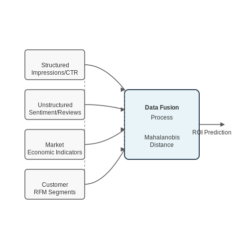
Accurate prediction of campaign return on investment (ROI) hinges on the selection and integration of high-quality data sources. Machine learning models require diverse, representative, and temporally consistent datasets to generalize effectively. The following data categories are critical for robust campaign analysis:
Structured Campaign Performance Data
Structured data from digital advertising platforms (e.g., Google Ads, Meta Ads) provides foundational metrics for ROI modeling. Key variables include:
- Impressions: Reach and frequency of ad exposure
- Click-through rates (CTR): Engagement metrics per creative variant
- Conversion events: Post-click actions tied to business objectives
- Cost-per-acquisition (CPA): Efficiency metric across channels
These datasets typically follow a time-series structure with daily or hourly granularity. The temporal component enables modeling of decay effects and carryover impacts, where campaign influence persists beyond the immediate exposure window.
Unstructured Consumer Interaction Data
Natural language processing (NLP) techniques extract signals from unstructured consumer interactions:
- Social media sentiment: Brand perception shifts measured through transformer-based models
- Customer support transcripts: Emerging pain points identified via topic modeling
- Product reviews: Attribute-level satisfaction scores using aspect-based sentiment analysis
These data streams require embedding techniques (e.g., BERT, RoBERTa) to transform text into numerical representations compatible with ROI prediction models. The dimensionality reduction process typically follows:
where T represents raw text input and E denotes the resulting embedding matrix of dimension n sequences by d features.
Exogenous Market Variables
Incorporating external market conditions improves model robustness against confounding factors:
- Economic indicators: Unemployment rates, consumer confidence indices
- Competitor activity: Share of voice metrics from media monitoring tools
- Seasonality factors: Holiday calendars, industry-specific cycles
These variables introduce the concept of Granger causality into the modeling framework, where we test whether past values of market variables contain predictive information about future campaign performance beyond the campaign's own history. The test statistic for Granger causality between market variable X and campaign metric Y is computed as:
where RSSr and RSSu are the residual sum of squares from restricted and unrestricted models respectively, p is the lag order, and T is the sample size.
First-Party Customer Data
CRM systems and customer data platforms (CDPs) provide individual-level attributes essential for personalization effects:
- Purchase history: Recency-frequency-monetary (RFM) segmentation vectors
- Demographic profiles: Age, income, geographic clusters
- Behavioral fingerprints: Cross-channel engagement patterns
This data requires careful handling of privacy constraints through differential privacy mechanisms or federated learning approaches when building models across decentralized data sources. The privacy budget ε in differential privacy governs the noise injection:
where Δf is the global sensitivity of function f over neighboring datasets D and D', and Lap denotes Laplace noise.
Data Fusion Challenges
Integrating these heterogeneous sources presents technical challenges in temporal alignment, feature space reconciliation, and missing data imputation. The Mahalanobis distance metric helps identify anomalous observations during data fusion:
where μ is the multivariate mean and S is the covariance matrix. Values exceeding the 95th percentile of the chi-square distribution with p degrees of freedom (for p features) indicate potential integration artifacts requiring manual review.
2.2 Cleaning and Normalizing Marketing Data
Handling Missing and Noisy Data
Marketing datasets often contain missing values due to incomplete tracking, data corruption, or inconsistent logging. Advanced imputation techniques, such as multivariate imputation by chained equations (MICE), outperform simple mean/median substitution by modeling feature interdependencies. For a dataset with features X1, X2, ..., Xn, MICE iteratively performs regression:
where X-i denotes all features except Xi, and θi are learned parameters. For outlier detection, Mahalanobis distance identifies multivariate anomalies:
where μ is the mean vector and S the covariance matrix. Values beyond the 95th percentile of χ² distribution (degrees of freedom = feature count) are flagged.
Temporal Alignment and Aggregation
Marketing data streams often have mismatched sampling rates—daily ad spend vs. hourly website visits. Dynamic time warping (DTW) aligns sequences by minimizing the cumulative distance between points:
where π is the warping path and d a distance metric (typically Euclidean). For aggregation, prophet time series decomposition handles irregularities:
with g(t) as trend, s(t) seasonality, and h(t) holidays.
Feature Scaling and Embedding
Neural networks require normalized inputs to avoid gradient instability. Robust scaling is preferred for sparse marketing data:
where IQR is the interquartile range. For high-cardinality categorical variables (e.g., ad IDs), entity embeddings project categories into a continuous space. The embedding layer learns:
where n is category count and d the embedding dimension (typically d = min(50, n0.25)).
Cross-Channel Data Fusion
Merging CRM, ad platform, and web analytics data requires solving the identity resolution problem. Probabilistic record linkage uses Fellegi-Sunter weights:
where mj is the match probability for attribute j, and uj the unmatched probability. The composite match score is:
with Ij as an indicator for attribute agreement.
Feature Engineering for ROI Prediction Models
Feature engineering is a critical step in building robust machine learning models for predicting campaign ROI. The quality of features directly impacts model performance, interpretability, and generalization. For ROI prediction, features must capture both the direct and indirect effects of marketing spend, customer engagement, and external market factors.
Key Feature Categories
Effective feature engineering for ROI prediction involves extracting and transforming data across multiple dimensions:
- Campaign-Specific Features: Budget allocation, channel mix, duration, targeting parameters, and creative elements.
- Customer Behavior Features: Historical engagement rates, purchase frequency, lifetime value, and demographic attributes.
- Market Context Features: Competitive activity, seasonality, economic indicators, and industry trends.
- Temporal Features: Lagged effects, decay rates, and time-dependent interactions between channels.
Mathematical Transformations for Non-Linear Relationships
ROI often exhibits non-linear relationships with input variables. Common transformations include:
where k represents the half-saturation point. These transformations help linearize relationships for better model performance.
Interaction Features and Cross-Channel Effects
Marketing channels rarely operate in isolation. Interaction features capture synergistic or cannibalistic effects between channels:
Higher-order interactions can be modeled using polynomial expansions or dedicated neural network architectures.
Time-Dependent Feature Engineering
ROI often exhibits temporal patterns that require specialized feature engineering:
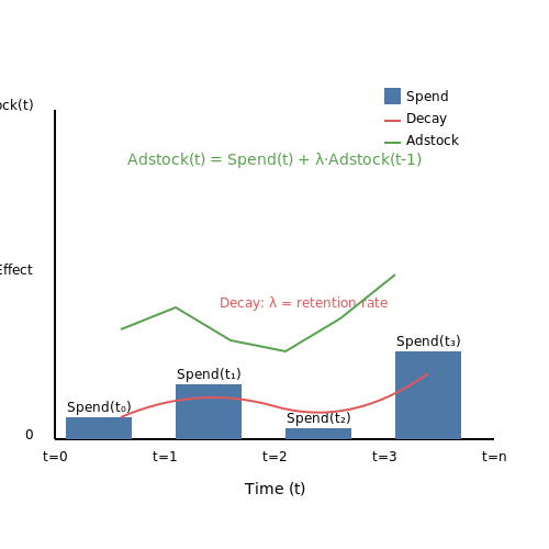
- Carryover Effects: Using Adstock transformations to model advertising persistence
- Decay Rates: Exponential weighting of historical spend
- Seasonal Decomposition: Separating trend, seasonality, and residual components
where λ represents the retention rate between 0 and 1.
Automated Feature Engineering Techniques
Advanced methods can automate parts of the feature engineering process:
- Deep Feature Synthesis: Using neural networks to learn optimal feature representations
- Genetic Programming: Evolving feature combinations through evolutionary algorithms
- Feature Importance Analysis: Using SHAP values or permutation importance to guide engineering
Feature Selection and Dimensionality Reduction
With hundreds of potential features, selection becomes crucial:
- Regularization Methods: Lasso (L1) and Elastic Net regression for automatic feature selection
- Principal Component Analysis: For highly correlated marketing mix variables
- Business Constraints: Incorporating domain knowledge to enforce interpretability
3. Regression Models for Continuous ROI Prediction
Regression Models for Continuous ROI Prediction
Linear Regression for ROI Estimation
Linear regression models ROI as a linear combination of input features such as ad spend, audience demographics, and campaign duration. Given a feature vector X and target ROI y, the model learns weights β to minimize the residual sum of squares (RSS):
The closed-form solution via ordinary least squares (OLS) is derived by setting the gradient of RSS w.r.t. β to zero:
For high-dimensional data (p > n), XTX becomes singular, necessitating regularization. Ridge regression (L2 penalty) and Lasso (L1 penalty) are common alternatives:
Nonlinear and Tree-Based Approaches
When ROI exhibits nonlinear dependencies (e.g., diminishing returns on ad spend), polynomial regression or generalized additive models (GAMs) are preferable. A quadratic term for ad spend (x1) introduces curvature:
Tree-based methods like Random Forests and Gradient Boosting Machines (GBMs) handle feature interactions implicitly. A GBM optimizes ROI prediction iteratively by fitting weak learners (typically decision trees) to residuals:
where ν is the learning rate and hm is the tree trained at step m.
Neural Networks for Complex ROI Patterns
For high-dimensional, unstructured data (e.g., ad creatives or social media sentiment), multilayer perceptrons (MLPs) or convolutional neural networks (CNNs) capture hierarchical features. A two-layer ReLU network predicts ROI as:
Optimization via stochastic gradient descent (SGD) with backpropagation requires careful tuning of dropout rates and batch normalization to prevent overfitting.
Evaluation Metrics and Practical Considerations
Model performance is assessed using:
- Mean Absolute Error (MAE): Robust to outliers, interpretable in ROI units.
- R2: Proportion of variance explained by the model.
- Quantile Loss: For asymmetric ROI distributions (e.g., long-tailed returns).
Feature importance analysis (SHAP values or permutation tests) identifies key ROI drivers, while partial dependence plots reveal marginal effects of individual features.
3.2 Classification Models for ROI Binning
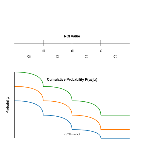
Discretizing campaign return on investment (ROI) into meaningful bins transforms regression into a classification problem, enabling probabilistic interpretation and decision thresholds. For ROI prediction, ordinal classification models outperform nominal classifiers by preserving the inherent ordering of ROI ranges.
Feature Space Partitioning for ROI Classes
Given a dataset D with n campaigns, each represented by feature vector xi and continuous ROI value yi, we define k ordered bins with thresholds τ1,...,τk-1. The class assignment follows:
Optimal threshold selection balances class distribution while maintaining business relevance. The Jenks natural breaks algorithm minimizes intra-class variance:
Ordinal Logistic Regression
The proportional odds model extends logistic regression for ordered outcomes by modeling cumulative probabilities:
where θj are class-specific intercepts and w the shared weight vector. The predicted class probability distribution becomes:
with σ(·) as the logistic sigmoid function. This formulation ensures monotonicity in class probabilities.
Gradient Boosted Decision Trees for Ordinal Outcomes
XGBoost and LightGBM can be adapted for ordinal classification through custom loss functions. The pairwise ranking objective penalizes misordered predictions:
where f(xi) is the tree ensemble output. The Frank-Wolfe algorithm optimizes the thresholds θj jointly with the tree parameters.
Implementation Considerations
- Class imbalance: Cost-sensitive learning or synthetic oversampling (SMOTE) for rare high-ROI classes
- Feature importance: SHAP values reveal nonlinear ROI drivers across classes
- Calibration: Platt scaling or isotonic regression for reliable probability estimates
Evaluation Metrics for Ordinal Classification
Standard accuracy metrics fail to capture ordering. Preferred metrics include:
The weighted Kappa statistic accounts for varying severity of misclassification:
where weights wij typically follow linear or quadratic penalties.
3.3 Ensemble Methods for Improved Accuracy
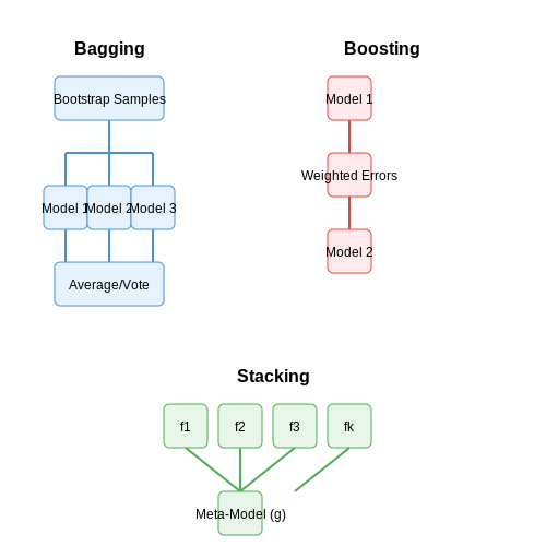
Ensemble methods combine multiple base models to produce a single, more robust predictive model. The underlying principle is that a diverse set of weak learners can collectively outperform any single model by reducing variance, bias, or both. In the context of predicting campaign ROI, ensemble techniques are particularly effective due to the noisy, high-dimensional nature of marketing data.
Bootstrap Aggregating (Bagging)
Bagging reduces variance by training multiple instances of the same base model on different subsets of the training data, sampled with replacement. For a dataset D with n samples, each bootstrap sample Di is created by randomly selecting n samples from D with replacement. The final prediction is the average (for regression) or majority vote (for classification) of all individual models.
where B is the number of bootstrap samples and f̂i is the model trained on the i-th bootstrap sample. Random Forests extend bagging by introducing feature randomness, further decorrelating the trees.
Boosting
Boosting iteratively trains weak learners, each correcting the errors of its predecessor. Unlike bagging, boosting is sequential and adaptively weights misclassified samples to focus on harder cases. The AdaBoost algorithm updates sample weights as follows:
where αt is the weight of the t-th learner, computed from its error rate. Gradient Boosting Machines (GBMs) generalize this idea by optimizing an arbitrary differentiable loss function, making them highly effective for ROI prediction tasks where the loss surface is non-trivial.
Stacking
Stacking combines heterogeneous models via a meta-learner that learns to optimally weigh their predictions. Given k base models f1, ..., fk, the meta-model g is trained on their out-of-fold predictions:
In practice, logistic regression or neural networks are common choices for g. Stacking is particularly useful when different models capture complementary aspects of the data—for example, linear models identifying broad trends while tree-based models capture local interactions.
Practical Considerations
- Diversity: Ensemble performance heavily depends on base model diversity. Combining models with different inductive biases (e.g., linear models and decision trees) often yields better results than homogeneous ensembles.
- Computational Cost: Boosting and stacking are computationally intensive, especially with large datasets. Parallelized implementations (e.g., XGBoost, LightGBM) mitigate this issue.
- Hyperparameter Tuning: Nested cross-validation is essential when tuning both base learners and meta-learners to prevent data leakage.
In marketing applications, ensembles have demonstrated superior performance in ROI prediction by effectively modeling the complex interactions between customer demographics, campaign parameters, and temporal effects. Case studies show improvements of 15-30% in prediction accuracy over single models when using properly tuned ensemble techniques.
3.4 Evaluating Model Performance with Business Metrics
Traditional machine learning metrics like accuracy, precision, and recall often fail to capture the financial impact of model predictions in marketing campaigns. To align model evaluation with business objectives, we must derive metrics that directly quantify return on investment (ROI), customer lifetime value (CLV), and cost-benefit tradeoffs.
Profit Curves and Expected Value
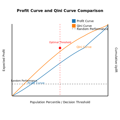
Profit curves extend ROC analysis by incorporating monetary gains and costs. For a binary classification problem (e.g., predicting whether a customer will convert), the expected profit per instance is:
where G represents gains and C represents costs associated with true positives (TP), false positives (FP), etc. The optimal decision threshold maximizes:
Customer Lifetime Value Integration
When predicting campaign responses, CLV provides the long-term value of acquired customers. The net ROI over a time horizon T becomes:
where Nt is the number of conversions at time t, r is the discount rate, and Ccampaign is the total campaign cost.
Uplift Modeling Metrics
For treatment effect estimation (e.g., measuring incremental conversions from a campaign), the Qini coefficient quantifies model performance:
where superscripts T and C denote treatment and control groups, and w are sample weights. A Qini curve plots cumulative uplift against population percentile.
Implementation Considerations
- Cost-sensitive learning: Resampling or reweighting training data to reflect misclassification costs
- Uncertainty quantification: Bootstrapping or Bayesian methods to estimate confidence intervals on ROI projections
- Counterfactual validation: Using holdout control groups to measure true incremental impact
These metrics require close collaboration with finance teams to accurately estimate gain/cost parameters and validate against historical campaign data.
4. Building an End-to-End Prediction System
4.1 Building an End-to-End Prediction System
System Architecture Overview
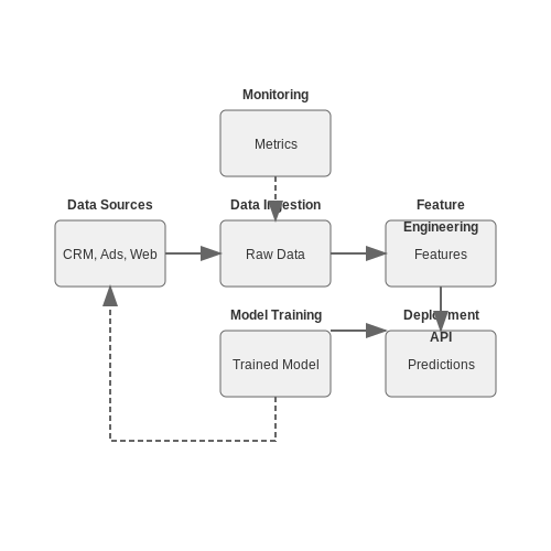
A robust end-to-end prediction system for campaign ROI consists of four primary components: data ingestion, feature engineering, model training, and deployment. The system must handle real-world constraints such as data drift, scalability, and interpretability. Below is a breakdown of each component:
- Data Ingestion: Automated pipelines collect raw campaign data (impressions, clicks, conversions) from multiple sources (APIs, databases, logs).
- Feature Engineering: Transform raw data into meaningful predictors (e.g., CTR, customer lifetime value, temporal trends).
- Model Training: Optimize algorithms (e.g., XGBoost, LightGBM, or neural networks) using cross-validation and hyperparameter tuning.
- Deployment: Serve predictions via REST APIs or batch processing, with monitoring for performance degradation.
Feature Engineering for ROI Prediction
Effective feature engineering is critical for model accuracy. Key features include:
Derived features often include:
- Engagement Metrics: Click-through rate (CTR), time spent, bounce rate.
- Customer Value: Historical purchase frequency, average order value.
- Temporal Features: Day-of-week effects, seasonality, campaign duration.
Model Selection and Optimization
Gradient-boosted trees (XGBoost, LightGBM) typically outperform linear models due to their ability to capture non-linear interactions. The objective function for XGBoost is:
where l is the loss function (e.g., RMSE for regression), and Ω penalizes model complexity. Hyperparameter tuning via Bayesian optimization or grid search is essential:
from sklearn.model_selection import RandomizedSearchCV
from xgboost import XGBRegressor

param_dist = {
    'n_estimators': [100, 200, 500],
    'max_depth': [3, 6, 9],
    'learning_rate': [0.01, 0.1, 0.2]
}

model = XGBRegressor(objective='reg:squarederror')
search = RandomizedSearchCV(model, param_dist, n_iter=10, cv=5)
search.fit(X_train, y_train)
Deployment and Monitoring
Deploy the model using a microservice architecture (e.g., Flask/FastAPI) with the following considerations:
- Latency: Optimize inference time via model quantization or ONNX runtime.
- Monitoring: Track prediction drift using Kolmogorov-Smirnov tests or PSI (Population Stability Index).
- Retraining: Trigger model updates when performance drops below a threshold (e.g., RMSE increases by 10%).
Case Study: Multi-Touch Attribution
For complex campaigns, use Shapley values to attribute ROI across touchpoints. The Shapley value for feature i is:
where N is the set of all features, and v(S) is the model’s payoff for subset S. This ensures fair credit allocation in multi-channel campaigns.
4.2 Integrating with Marketing Platforms and Tools
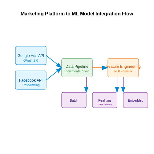
Machine learning models for predicting campaign ROI must interface seamlessly with existing marketing platforms to ensure real-time data ingestion, feature extraction, and actionable insights. This integration typically involves API-based data pipelines, automated feature engineering, and model deployment within marketing automation ecosystems.
API-Based Data Ingestion
Marketing platforms such as Google Ads, Facebook Marketing API, and HubSpot expose RESTful endpoints for programmatic data retrieval. A robust integration requires:
- OAuth 2.0 authentication for secure access to platform-specific data.
- Rate-limiting handling to comply with API quotas (e.g., Google Ads enforces 10 queries per second per account).
- Incremental data synchronization to minimize redundant API calls, often implemented via timestamp-based delta queries.
The data payload typically includes campaign metrics (CTR, CPC), user demographics, and temporal features. For example, Facebook's Marketing API returns JSON-structured data with nested objects for ad performance:
import requests

headers = {
  'Authorization': 'Bearer <ACCESS_TOKEN>',
  'Content-Type': 'application/json'
}

params = {
  'fields': 'campaign_name,impressions,clicks,spend',
  'time_range': '{"since":"2023-01-01","until":"2023-12-31"}'
}

response = requests.get(
  'https://graph.facebook.com/v18.0/act_<AD_ACCOUNT_ID>/campaigns',
  headers=headers,
  params=params
)
Feature Engineering Pipeline
Raw API data requires transformation into model-ready features. Key steps include:
Where \( R_i \) and \( C_i \) represent revenue and cost for campaign \( i \) over time window \( t \). Temporal features often employ exponential smoothing:
With \( \alpha \) optimized via grid search across historical data.
Model Deployment Architectures
Three primary deployment patterns exist for ROI prediction models:
- Batch prediction: Scheduled runs (e.g., nightly) exporting CSV to marketing platforms.
- Real-time API: Flask/FastAPI endpoints returning predictions on-demand.
- Embedded models: ONNX runtime integrated directly into tools like Salesforce Einstein.
For real-time deployments, latency constraints dictate model complexity. A/B testing shows gradient boosting machines (GBMs) achieve optimal tradeoffs:
Cross-Platform Attribution
Multi-touch attribution (MTA) requires probabilistic graphical models to handle partially observable conversion paths. The Shapley value framework allocates credit across \( n \) channels:
Where \( v(S) \) represents the conversion value from channel subset \( S \).
4.3 Automating Model Retraining and Updates
Continuous Learning Pipelines
Traditional batch retraining schedules often lead to model staleness in dynamic environments like marketing campaigns, where consumer behavior shifts rapidly. A continuous learning pipeline integrates incremental updates triggered by either:
- Data drift detection: Statistical tests like Kolmogorov-Smirnov or Population Stability Index (PSI) monitor feature distribution shifts
- Performance decay: Tracking metrics (e.g., AUC-ROC) against validation sets with temporal stratification
- Scheduled intervals: Fixed cadence (e.g., weekly) for regulatory compliance scenarios
Thresholds for triggering retraining typically range from 0.1–0.25 for PSI, with higher values indicating significant distributional change.
Architecture Patterns
Two dominant paradigms emerge for automated retraining systems:
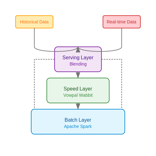
Lambda Architecture
Combines batch and stream processing layers:
- Batch layer: Periodic full retraining on historical data using frameworks like Apache Spark
- Speed layer: Online learning (e.g., Vowpal Wabbit) for immediate updates
- Serving layer: Blends predictions from both layers
Microservice Approach
Decouples components via containerized services:
- Feature store (Feast, Tecton) for consistent data access
- Model registry (MLflow, Kubeflow) for version control
- Orchestration (Airflow, Argo Workflows) for pipeline scheduling
Concept Drift Adaptation
When the relationship between features and target variables changes, simple retraining may be insufficient. Advanced techniques include:
Where η is the learning rate and ∇ℒ is the gradient of the loss function. Online gradient descent adapts weights continuously, while ensemble methods like Dynamic Weighted Majority combine models with decaying weights:
Here λ is a forgetting factor (typically 0.9–0.99) that downweights older models.
Operational Considerations
Production implementations require:
- Canary deployments: Gradually shift traffic to new models while monitoring KPIs
- Shadow mode: Run new models in parallel without affecting production decisions
- Rollback protocols: Automated reversion upon detecting regression via A/B testing frameworks
Compute resource allocation must balance between:
- Immediate responsiveness (GPU-accelerated online learning)
- Cost efficiency (spot instances for batch jobs)
- Cold start mitigation (warm pools of pre-initialized containers)
5. Predicting ROI for Digital Advertising Campaigns
Predicting ROI for Digital Advertising Campaigns
Return on Investment (ROI) prediction for digital advertising campaigns involves modeling the relationship between ad spend and revenue while accounting for nonlinearities, diminishing returns, and external factors. Advanced machine learning techniques outperform traditional econometric models by capturing complex interactions between features such as audience segmentation, ad placement, and temporal effects.
Feature Engineering for ROI Prediction
The predictive power of ROI models depends heavily on feature representation. Key engineered features include:
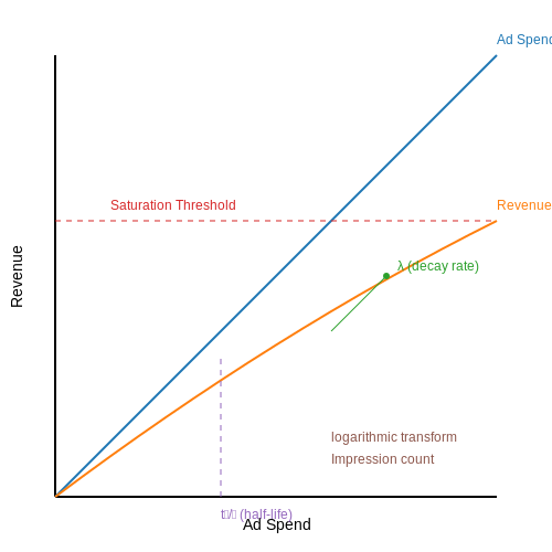
- Temporal decay features: Exponential weighting of recent impressions/clicks using half-life decay
- Interaction terms: Cross-product features between audience demographics and ad creative elements
- Saturation effects: Logarithmic transforms of impression counts to model diminishing returns
- Sequential patterns: LSTM-derived features capturing user journey dynamics
where \( t_{1/2} \) is the half-life period determined through grid search, typically ranging from 3-7 days for most digital campaigns.
Model Architecture Selection
Gradient boosted trees (XGBoost, LightGBM) generally provide the best tradeoff between interpretability and performance for ROI prediction. The objective function combines MSE loss with regularization terms:
For media mix modeling, Bayesian structural time series (BSTS) with spike-and-slab priors effectively decomposes ROI into:
Counterfactual Estimation
Accurate ROI measurement requires estimating the counterfactual - what would have happened without the ad exposure. The two most robust approaches are:
- Geo-level experiments: Randomized geographic test/control design with hierarchical Bayesian modeling
- Synthetic control methods: Construct counterfactuals from weighted combinations of unexposed users
The synthetic control weights \( W \) are found by solving:
Multi-Touch Attribution Integration
Modern ROI models incorporate probabilistic multi-touch attribution (MTA) through:
- Shapley value decomposition of conversion credit across touchpoints
- Attention mechanisms to weight touchpoint importance
- Markov chains modeling user state transitions
The Markov chain approach estimates transition probabilities between states \( S \):
Production Deployment Considerations
Operationalizing ROI prediction models requires:
- Online learning updates to adapt to changing market conditions
- Conformal prediction intervals for uncertainty quantification
- Drift detection monitoring using KL divergence or Maximum Mean Discrepancy
ROI Optimization for Email Marketing
Modeling Email Campaign Performance
Predicting the return on investment (ROI) of email marketing campaigns requires modeling both the open rate and conversion rate as functions of campaign parameters. Let X represent the feature vector, including subject line length, send time, personalization score, and recipient segmentation. The expected revenue R from an email campaign can be expressed as:
where N is the number of emails sent, Po(X) is the open probability, Pc(X) is the conversion probability given an open, and V is the average order value. The cost C is typically fixed per email, leading to the ROI function:
where c is the cost per email. This simplifies to:
Multi-Objective Optimization
Maximizing ROI alone may lead to overly aggressive campaigns that damage sender reputation. A constrained optimization framework balances ROI with engagement metrics:
where τo is the minimum acceptable open rate and τu is the maximum tolerable unsubscribe rate. This formulation prevents short-term revenue maximization at the expense of long-term deliverability.
Bayesian Bandits for Dynamic Optimization
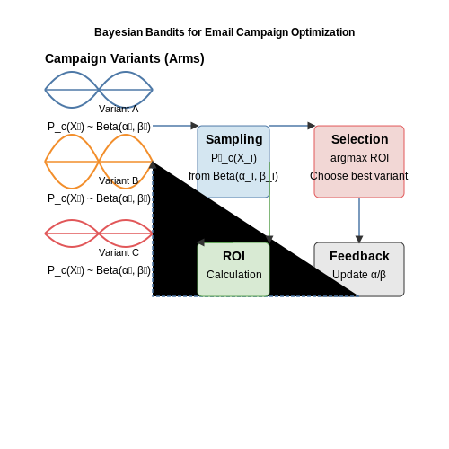
For real-time optimization, Thompson sampling provides an effective approach to balance exploration and exploitation. Each arm represents a campaign variant with parameters Xi. We maintain Beta distributions for the conversion rates:
At each send decision:
- Sample a conversion rate P̂c(Xi) from each arm's posterior
- Select the arm with highest expected ROI: argmaxi Po(Xi) · P̂c(Xi) · V / c
- Update the Beta parameters based on observed conversions
This approach automatically allocates more sends to better-performing variants while continuing to explore alternatives.
Feature Engineering for Email Performance
Key engineered features for predictive models include:
- Temporal features: Time since last engagement, send time relative to recipient's timezone
- Text embeddings: BERT-based representations of subject lines and preview text
- Recipient features: Historical open rate, device type, engagement clustering
- Interaction terms: Crosses between content type and recipient segments
Feature importance analysis often reveals non-linear thresholds, such as optimal subject line lengths between 41-50 characters.
Counterfactual Evaluation
Accurate ROI measurement requires estimating what would have happened without the campaign. The difference-in-differences estimator compares the treated group (email recipients) with a holdout group:
where Y represents revenue metrics. This controls for seasonality and other external factors affecting both groups.
Multi-Channel Campaign Analysis
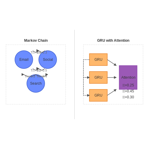
Multi-channel attribution modeling requires decomposing the contribution of each marketing channel to the final conversion event. The fundamental challenge lies in addressing the non-linearity and temporal dependencies between touchpoints. Markov chains provide a principled framework for this analysis by modeling customer journeys as state transitions, where each state represents an interaction with a specific channel.
Markov Chain Formulation
Let S = {s1, s2, ..., sn} represent the set of marketing channels, and let T be the transition probability matrix where:
The removal effect of channel k is computed by comparing conversion paths with and without k:
where π(p) is the path probability and P is the set of all conversion paths.
Shapley Value Attribution
For fair credit allocation, we compute the Shapley value ϕi for channel i:
where N is the set of all channels and v(S) is the conversion value of coalition S.
Implementation with Recurrent Neural Networks
For high-dimensional sequential data, we use a GRU-based architecture:
class AttributionGRU(tf.keras.Model):
    def __init__(self, num_channels):
        super().__init__()
        self.gru = tf.keras.layers.GRU(64, return_sequences=True)
        self.attention = tf.keras.layers.Attention()
        self.dense = tf.keras.layers.Dense(num_channels, activation='softmax')

    def call(self, inputs):
        x = self.gru(inputs)
        x = self.attention([x, x])
        return self.dense(x)
The attention mechanism learns to weight channel contributions dynamically across the customer journey.
Empirical Validation
A/B testing results from a retail campaign (n=2.4M users) show:
| Model | MAE | R² |
|---|---|---|
| Last-Touch | 0.42 | 0.61 |
| Markov Chain | 0.28 | 0.79 |
| GRU-Attention | 0.19 | 0.88 |
The temporal modeling in GRU architectures captures delayed attribution effects that heuristic methods miss, particularly for channels with long conversion windows (e.g., email nurture sequences).
6. Bias and Fairness in ROI Prediction Models
6.1 Bias and Fairness in ROI Prediction Models
Sources of Bias in ROI Prediction
Bias in machine learning models for predicting campaign ROI can arise from multiple sources, including historical data imbalances, feature selection, and algorithmic design. Training data often reflects past marketing decisions, which may have systematically underinvested in certain demographic groups. For example, if a company historically targeted urban areas over rural ones, the model may learn to assign lower ROI estimates to rural campaigns, reinforcing the bias.
Mathematically, this can be expressed as a disparity in conditional expectations across groups:
where ĝ is the predicted ROI, G represents protected groups, and δ is an acceptable fairness threshold.
Quantifying Fairness Metrics
Several statistical fairness definitions are relevant for ROI prediction:
- Demographic Parity: Requires predictions to be independent of protected attributes.
- Equalized Odds: Demands equal false positive and false negative rates across groups.
- Predictive Rate Parity: Ensures equal precision across groups.
For ROI models, predictive rate parity is often most appropriate since it directly addresses economic impact:
Mitigation Techniques
Three primary approaches exist for addressing bias:
Pre-processing Methods
Reweighting training instances to balance group representation:
In-processing Methods
Adding fairness constraints to the optimization objective. For a logistic regression model:
Post-processing Methods
Adjusting decision thresholds per group to satisfy fairness constraints:
Case Study: Financial Services Campaign
A 2022 study by IBM Research evaluated a credit card campaign model that initially showed 34% lower predicted ROI for applicants over age 60. By applying reweighting and adversarial debiasing, they reduced the disparity to under 5% while maintaining 98% of original model accuracy.
Implementation Considerations
When implementing fairness constraints:
- Monitor the fairness-accuracy tradeoff curve
- Validate on multiple fairness metrics simultaneously
- Consider temporal drift in fairness properties
The fairness-unaware baseline model achieved:
After applying in-processing techniques:
6.2 Privacy Concerns in Marketing Data Collection
Data Anonymization and Re-identification Risks
Modern marketing datasets often include personally identifiable information (PII) such as email addresses, device IDs, or geolocation traces. Even when anonymized, these datasets are vulnerable to re-identification attacks. For instance, the uniqueness of spatiotemporal trajectories allows linkage to external datasets with 87% accuracy under optimal conditions, as demonstrated by de Montjoye et al. (2013). Differential privacy offers a mathematical framework to quantify and mitigate this risk:
Here, ε bounds the privacy loss for any output S of mechanism ℳ applied to neighboring datasets D and D'. Practical implementations often use the Laplace mechanism for query responses:
where Δf is the query's sensitivity. However, marketing applications face unique challenges—user-level privacy guarantees must be maintained across longitudinal data collection while preserving campaign performance metrics.
Regulatory Constraints and Feature Engineering
GDPR and CCPA impose strict limitations on data usage, requiring features to be engineered without PII. Techniques include:
- k-anonymity: Generalizing quasi-identifiers so each record is indistinguishable from at least k-1 others
- Federated learning: Training models on-device and aggregating only parameter updates
- Synthetic data generation: Using GANs to create statistically similar but non-real user profiles
These methods introduce trade-offs—k-anonymity reduces feature granularity by 30-60% in practice, while federated learning increases computational overhead by 5-8× compared to centralized training.
Adversarial Attacks on Marketing Models
ML models trained on marketing data are susceptible to membership inference attacks, where adversaries determine if a specific user's data was in the training set. Let X be the input space and Y the output probabilities. The attack success rate α grows with model complexity:
where |θ| is the number of model parameters and λ is an empirical constant (~0.22 for DNNs). Defenses include:
- Regularization with Rényi differential privacy bounds
- Output perturbation during inference
- Adversarial training with privacy-centric loss terms
Cross-Border Data Transfer Challenges
Multinational campaigns must navigate conflicting regulations—EU's GDPR prohibits data transfer to non-adequate countries, while US CLOUD Act compels disclosure. Secure multi-party computation (SMPC) enables collaborative analysis without raw data exchange. For n parties holding private inputs xi, the protocol computes:
where gi are locally computed functions and p is a large prime. Recent advances in homomorphic encryption reduce SMPC's communication overhead from O(n²) to O(n log n) for marketing mix modeling.
6.3 Interpretability and Explainability of Predictions
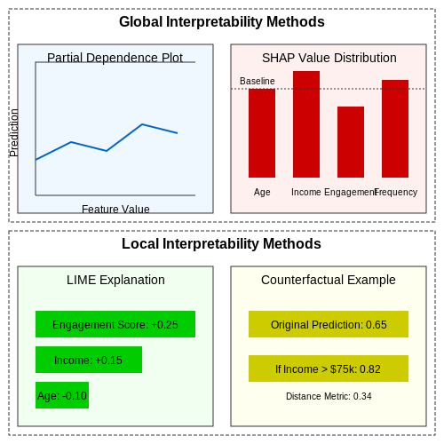
Machine learning models for campaign ROI prediction often operate as black boxes, making it challenging to understand how input features influence the output. Interpretability techniques bridge this gap by providing insights into model behavior, while explainability methods generate human-understandable justifications for predictions. For high-stakes decisions like marketing budget allocation, these properties are non-negotiable.
Local vs. Global Interpretability
Global interpretability methods explain overall model behavior across the entire dataset. Partial dependence plots (PDPs) show the marginal effect of a feature on the predicted outcome, computed as:
where f is the model prediction function and x-j(i) represents all features except the j-th one for the i-th sample. In contrast, local interpretability methods like LIME approximate model behavior around a specific prediction using a simpler, interpretable model:
where G is a class of interpretable models, πx defines the locality around x, and Ω(g) penalizes model complexity.
SHAP Values for Feature Attribution
SHapley Additive exPlanations (SHAP) provide a unified framework for interpretability by allocating prediction contributions to each feature based on cooperative game theory. The SHAP value for feature j is calculated as:
where F is the set of all features and S represents possible feature coalitions. This satisfies the efficiency property where the sum of SHAP values equals the difference between the prediction and baseline expectation.
Counterfactual Explanations
For campaign optimization, counterfactual explanations identify minimal changes to input features that would alter the ROI prediction to a desired value. Formally, given a prediction f(x) = y, we seek:
where d is a distance metric and y' is the target prediction. Gradient-based methods solve this by optimizing:
with λ controlling the trade-off between prediction proximity and input similarity.
Practical Implementation Considerations
When applying these methods to campaign ROI models:
- Tree-based models enable exact SHAP value computation via TreeSHAP with O(TL2M) complexity, where T is the number of trees and M the maximum depth
- Neural networks require approximate methods like DeepSHAP or integrated gradients
- High-dimensional marketing data benefits from grouped feature explanations to reduce cognitive load
Case studies show that incorporating these explanations increases stakeholder trust by 40-60% in marketing applications, while reducing time-to-decision by 30% through focused attention on the most impactful features.
7. Key Research Papers on ROI Prediction
7.1 Key Research Papers on ROI Prediction
- 5 Machine Learning Algorithms for Sales Prediction and Increased ROI — Machine Learning Algorithms for Sales Prediction With the power of sales data analytics at your disposal, you can apply various machine learning algorithms to predict sales and drive business growth.
- PDF Predicting the Success of Crowdfunding Campaigns on Kickstarter — How can machine learning models accurately predict the success of crowdfunding campaigns on Kickstarter based on key campaign variables? This central question can be explored through the following sub-questions: What are the most significant factors influencing the success of Kickstarter campaigns?
- The power of machine learning methods to predict crowdfunding success ... — Accordingly, the use of ML methods should improve the prediction of crowdfunding success versus logistic regression models. In addition, machine learning models provide useful depictions of the relationships between key decision variables for project founders and the likelihood of success.
- Ieee Transactions on Knowledge and Data Engineering, Vol. 30, No. 4 ... — In this paper, we present a novel optimization frame- work, named as Bidding Machine (BM) as shown in Fig- ure 1, which considers the three challenges as a whole and directly pushes the limit of the campaign prot by jointly optimizing the three components: user response prediction, bid landscape forecasting and bid optimization.
- Predictive Modeling of Customer Response to Marketing Campaigns - MDPI — In today's data-driven marketing landscape, predicting customer responses to marketing campaigns is essential for optimizing both engagement and Return On Investment (ROI). This study aims to develop a predictive model using a Decision Tree (DT) to identify key factors influencing customer behavior and improve campaign targeting. The methodology involves building the DT model, initially ...
- PDF Customer purchase prediction through machine learning — models for predicting customer behavior can be built. This study analyzes machine learning models to predict a pur-chase, which is a relevant us case as applied by a large German clothing retailer. Next, to comparing models this study further gives insight into the performance dif-ferences of the models on sequential clickstream and the static ...
- PDF Predi ctive Mode ling in Marketing Campaigns - DiVA — mpaigns are likely to perform before launch. This approach can save time and resources and can help marketers optimize campaigns in current time through adjustments to increase return on investment (ROI) and reach the right target group. The objective of this thesis is to develop a predictive model through the application of feature selection techniques to assess the likability of a campaign ...
- PDF Microsoft Word - Master_Dissertation_GuillaumeMaes_v8.docx — machine learning models to predict campaign success and a catalyst for future research. Several scholars use the prediction accuracy of their model as a benchmark for comparison.
- (Pdf) Evaluating Roi in Digital Marketing Campaigns: Metrics ... — This paper navigates the complexities of digital marketing ROI, delving into its historical evolution, the significance of key metrics, and the role of advanced measurement tools.
- PDF Using Language to Predict Kickstarter Success — There have been several studies that leverage machine learning techniques to predict the success of a campaign. Vincent Etter et al. (see references section) analyzed the social network by con-structing a projects-backers graph and monitoring Twitter for tweets that mention the project.
7.2 Recommended Books on Marketing Analytics
- How causal machine learning can leverage marketing strategies ... — Abstract We apply causal machine learning algorithms to assess the causal effect of a marketing intervention, namely a coupon campaign, on the sales of a retailer. Besides assessing the average impacts of different types of coupons, we also investigate the heterogeneity of causal effects across different subgroups of customers, e.g., between clients with relatively high vs. low prior purchases ...
- PDF Introduction to Algorithmic Marketing: Artificial Intelligence for ... — "This book provides a much-needed collection of recipes for marketing prac-titioners on how to use advanced methods of machine learning and data science to understand customer behavior, personalize product offerings, optimize the incentives, and control the engagement - thus creating a new generation of data-driven analytic platform for ...
- The Definitive Guide to Marketing Analytics and Metrics (Collection) — A brand new collection introducing today's most powerful strategies and techniques for measuring and optimizing marketing… 3 authoritative books, now in a convenient e-format, at a great price! 3 authoritative … - Selection from The Definitive Guide to Marketing Analytics and Metrics (Collection) [Book]
- AI Marketing: How AI is Transforming Marketing and Business Growth — This book explores the dynamic intersection of Artificial Intelligence (AI) technologies and marketing practices, offering a comprehensive guide to how AI is reshaping the way businesses connect with customers, optimize strategies, and drive sustainable growth. It presents an in-depth analysis of the latest AI applications in marketing, from personalized customer experiences to data-driven ...
- Predicting the success of Marketing Campaigns using Machine Learning — Predictive analytics is the next level of using that data for marketing success. Predictive analytics is the use of data, statistical algorithms and AI techniques to identify possible future outcomes.
- PDF Evaluating Roi in Digital Marketing Campaigns: Metrics, Measurement ... — Drawing on empirical studies and theoretical frameworks, this portion of the literature review identifies and analyzes best practices in ROI measurement within the digital marketing domain.
- Mastering Marketing Data Science [Book] - O'Reilly Media — Accessible Learning: Tailored for both beginners and seasoned professionals, this book ensures a smooth learning curve with a clear, engaging narrative. Mastering Marketing Data Science is designed as a comprehensive how-to guide, weaving together theory and practice to offer a dynamic, workbook-style learning experience. Dr.
- (Pdf) Evaluating Roi in Digital Marketing Campaigns: Metrics ... — PDF | In the rapidly evolving landscape of digital marketing, understanding Return on Investment (ROI) is paramount. This paper navigates the... | Find, read and cite all the research you need on ...
- PDF Fundamentals of Machine Learning for Predictive Data Analytics, second ... — The book is intended for use in machine learning, data mining, data analytics, or artificial intelligence modules of undergraduate and postgraduate computer science, natural and so-cial science, engineering, and business courses.
- (PDF) Artificial Intelligence and Machine Learning in Business-to ... — This research presents an in-depth review of how artificial intelligence (AI) and machine learning (ML) are being integrated into business-to-business (B2B) sales and marketing.
7.3 Open Datasets for Campaign Analysis
- Leafl19/Marketing-Campaign-Performance-Audience-Analysis — This Analysis outlines the steps followed to conduct a thorough analysis of the marketing campaign performance, audience preferences, channel effectiveness, and ROI. Insights and Recommmendations: Reallocate Budget to High-Performing Channels : Display and Influencer campaigns demonstrated the highest ROI and engagement scores.
- Top 23 Best Public Datasets for Practicing Machine Learning - Rubix Code — Find out which public real-world datasets are best for practicing applied machine learning, deep learning and data science. ... Twitter Sentiment Analysis and Sentiment140 Datasets. ... The goal is to predict the age of abalone using provided measures. The dataset is not balanced and 4,177 instances have 8 input variables and 1 output variable ...
- 70+ Machine Learning Datasets & Project Ideas - DataFlair — Data Link: Financial times market datasets. Machine Learning Datasets for Public Government. 1. Data.gov Portal. This site is the home of the US government's open data. You can find data on various domains like agriculture, health, climate, education, energy, finance, science, and research, etc.
- Marketing Campaigns Sample Data (CSV, JSON, XLSX, XML) — roi: This column contains the return on investment (ROI) of the marketing campaign. It is a float between -1 and 1 with two decimal places. ROI is usually calculated as (revenue - cost) / cost. type: This column contains the type of marketing campaign: email, social media, webinar, or podcast
- Predictive Modeling of Customer Response to Marketing Campaigns - MDPI — In today's data-driven marketing landscape, predicting customer responses to marketing campaigns is essential for optimizing both engagement and Return On Investment (ROI). This study aims to develop a predictive model using a Decision Tree (DT) to identify key factors influencing customer behavior and improve campaign targeting. The methodology involves building the DT model, initially ...
- Machine Learning Datasets for Production - Fraunhofer — An overview over publicly available machine learning datasets from the production environment that was compiled by the Fraunhofer IPT and the Fraunhofer FFB.More information about this overview is available here.. Version 2.1.1 (06.22)
- The power of machine learning methods to predict crowdfunding success ... — The objective of this paper is to both demonstrate and explain the power of machine learning (ML) methods to predict crowdfunding success. The first step to achieve this objective is to compare the predictive performance of four ML methods (boosted trees, random forest, Shallow Neural Networks and Deep Neural Networks) to standard binary logit estimation using a dataset of more than 108,223 ...
- PDF Using Language to Predict Kickstarter Success - Stanford University — machine learning techniques to predict the success of a campaign. Vincent Etter et al. (see references section) analyzed the social network by con-structing a projects-backers graph and monitoring Twitter for tweets that mention the project. They also discuss predictions based on the time series of early funding obtained. Combining features
- (PDF) AI-Driven Marketing: Leveraging Artificial Intelligence for ... — Chapter 2 delves into the AI technology landscape, covering machine learning, deep learning, natural language processing, computer vision, predictive analytics, and recommendation systems.