Hardware-Aware AI Model Training
1. Key Hardware Components Impacting Model Training
Key Hardware Components Impacting Model Training
GPU Architecture and Parallel Processing
Modern AI model training heavily relies on Graphics Processing Units (GPUs) due to their massively parallel architecture. Unlike CPUs, which excel at sequential tasks, GPUs consist of thousands of smaller, efficient cores designed for concurrent execution. The CUDA cores in NVIDIA GPUs, for instance, enable high-throughput floating-point operations (FLOPs), critical for matrix multiplications in deep learning. The memory bandwidth of GPUs, often exceeding 1 TB/s in high-end models like the A100, further accelerates data transfer between global memory and cores.
Tensor Cores, introduced in Volta and later architectures, optimize mixed-precision training by performing fused multiply-add (FMA) operations in a single clock cycle. For example, the operation:
is executed at 4x the speed of traditional FP32 operations when using FP16 inputs with FP32 accumulation.
Memory Hierarchy and Bandwidth
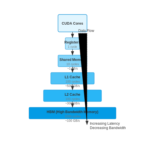
The memory hierarchy—comprising registers, shared memory, L1/L2 caches, and high-bandwidth memory (HBM)—plays a pivotal role in minimizing latency. HBM2e, used in GPUs like the H100, offers up to 3 TB/s bandwidth, reducing bottlenecks during gradient updates. The effective bandwidth (Beff) between device memory and compute units is given by:
Optimizing memory access patterns (e.g., coalesced reads in CUDA) can push Beff closer to the theoretical peak.
Interconnect Technologies
Multi-GPU training scales via NVLink (900 GB/s bidirectional bandwidth) and PCIe 5.0 (128 GB/s). The all-reduce operation in distributed training benefits from these interconnects, with communication time (Tcomm) modeled as:
where α is latency and β is the inverse bandwidth. NVLink’s lower α and higher bandwidth reduce Tcomm significantly compared to PCIe.
Specialized Accelerators
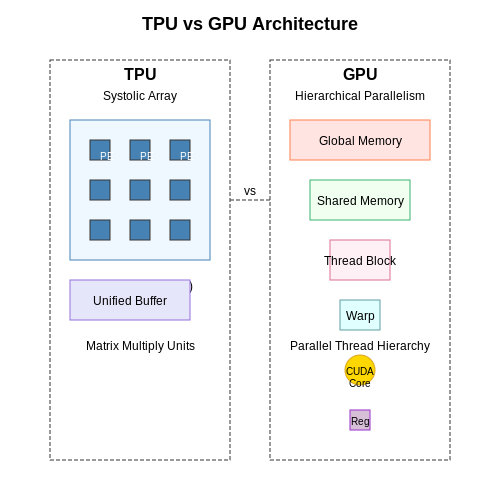
TPUs (Tensor Processing Units) leverage systolic arrays for dense matrix operations, optimizing the dataflow to avoid memory fetches. A TPU v4’s 128x128 systolic array performs 16K multiply-accumulate (MAC) operations per cycle, achieving 275 TFLOPS for bfloat16 precision. The energy efficiency (FLOPS/Watt) of TPUs often surpasses GPUs for large-scale transformer models.
Storage and Data Pipeline
NVMe SSDs (7 GB/s read speeds) and parallel filesystems (e.g., Lustre) prevent I/O bottlenecks during training. The data loading pipeline must saturate the GPU’s compute capacity, requiring optimizations like:
- Prefetching: Overlapping data loading with computation.
- Sharding: Distributing datasets across storage nodes.
The effective throughput (Tpipeline) of a data pipeline is constrained by the slowest stage (CPU decoding, storage I/O, or GPU compute):
Trade-offs Between Computational Resources and Model Performance
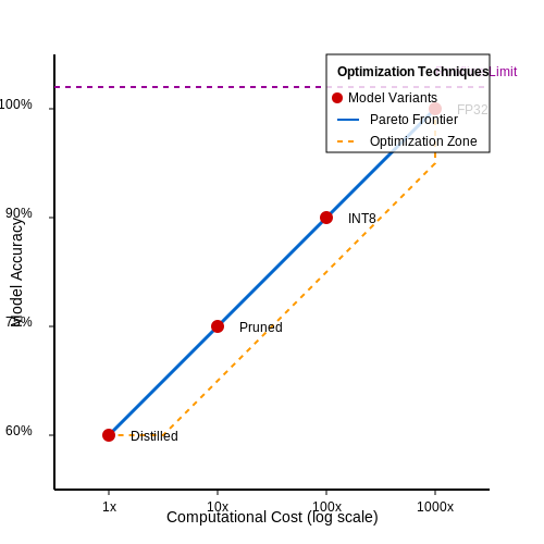
The relationship between computational resources and model performance is governed by a complex interplay of factors, including model architecture, optimization techniques, and hardware constraints. At the core of this trade-off lies the Pareto frontier, where improvements in one metric (e.g., accuracy) typically come at the expense of another (e.g., inference latency or memory footprint).
Quantifying the Trade-offs
The computational cost of training a neural network can be approximated by:
where N is the number of parameters, D is the dataset size, L is the number of layers, and B is the batch size. This relationship suggests that model complexity scales multiplicatively with each dimension of the problem.
Memory-Throughput Trade-off
Modern accelerators face a fundamental tension between memory bandwidth and computational throughput. The roofline model provides a framework for analyzing this:
where π is peak compute performance, β is memory bandwidth, and I is operational intensity (operations per byte transferred). This model reveals why certain architectures perform better on specific hardware configurations.
Practical Considerations in Model Design
- Pruning: Removing redundant weights can reduce model size by 90% with minimal accuracy loss, but requires careful iterative training
- Quantization: Moving from FP32 to INT8 can yield 4x memory savings and 2-3x speedup, but may require quantization-aware training
- Knowledge Distillation: Small models can achieve 90-95% of teacher model accuracy with proper distillation techniques
Hardware-Specific Optimization Strategies
Different hardware platforms impose distinct constraints:
| Hardware | Optimal Batch Size | Preferred Precision | Memory Hierarchy |
|---|---|---|---|
| GPUs | 32-256 | FP16/TF32 | Deep, wide |
| TPUs | 128-1024 | BF16 | Matrix-oriented |
| Edge TPUs | 1-8 | INT8 | Shallow, narrow |
Energy-Performance Trade-offs
The energy consumption of deep learning models follows a non-linear relationship with accuracy:
where coefficients α, β, and γ are hardware-dependent. This explains why model compression techniques often yield disproportionate energy savings compared to their theoretical FLOP reduction.
Case Study: Transformer Optimization
The evolution of transformer models illustrates these trade-offs clearly. While the original BERT model required 340MB of memory, distilled versions like TinyBERT achieve comparable performance with just 17MB. The optimization trajectory involves:
- Architecture search for optimal attention heads
- Dynamic sparse attention patterns
- Mixed-precision training
- Hardware-aware kernel fusion
Recent work has shown that careful co-design of algorithms and hardware can achieve 10-100x improvements in performance-per-watt compared to naive implementations.
Hardware Constraints in Edge vs. Cloud Environments
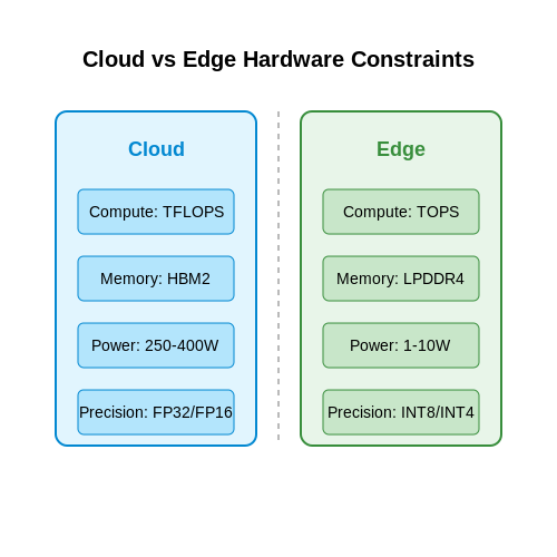
Edge and cloud computing environments impose fundamentally different hardware constraints on AI model training, necessitating distinct optimization strategies. The primary divergence stems from resource availability: cloud platforms leverage scalable, high-performance computing (HPC) infrastructure, while edge devices operate under strict power, memory, and thermal budgets.
Computational Throughput and Parallelism
Cloud environments typically employ GPUs or TPUs with thousands of cores, enabling massive parallelism for matrix operations. The theoretical peak performance for a modern GPU like the NVIDIA A100 can be calculated as:
For edge devices, ARM-based SoCs or specialized NPUs (e.g., Google Edge TPU) prioritize energy efficiency over raw throughput. Their performance follows:
Memory Hierarchy and Bandwidth
Cloud instances feature deep memory hierarchies with high-bandwidth interconnects (e.g., NVLink at 900GB/s). Edge devices rely on tightly coupled memory subsystems, where latency and power consumption dominate:
where C is capacitance, V is voltage, and f is access frequency. This necessitates model architectures with minimal off-chip memory access.
Thermal Design Power (TDP) Constraints
Cloud GPUs operate at 250-400W TDP, while edge devices are constrained to 1-10W. The thermal limit imposes a hard ceiling on sustained compute density:
Active cooling in cloud environments allows sustained peak performance, whereas passive edge cooling requires dynamic frequency scaling.
Quantization and Precision Tradeoffs
Cloud training typically uses FP32/FP16 precision, while edge inference employs INT8/INT4 quantization. The quantization error ε scales with:
where b is bit-width. This necessitates different approaches to maintaining model accuracy during hardware-aware training.
2. Quantization Techniques for Efficient Inference
Quantization Techniques for Efficient Inference
Fundamentals of Quantization
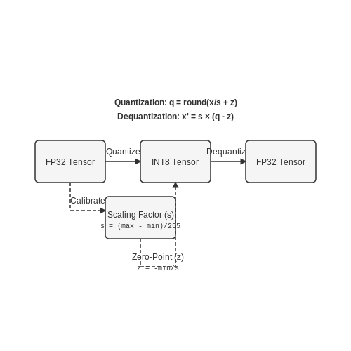
Quantization reduces the numerical precision of weights and activations in neural networks, enabling faster computation and lower memory footprint. The core idea involves mapping full-precision floating-point values (32-bit) to lower-bit integers (e.g., 8-bit). Given a floating-point tensor X, the quantized representation X̂ is computed as:
where s is the scaling factor and z is the zero-point, which maps the floating-point zero to an integer value. The scaling factor is derived from the tensor's dynamic range:
for n-bit quantization. The zero-point z ensures symmetric or asymmetric quantization, depending on whether the tensor's distribution is centered around zero.
Post-Training Quantization (PTQ)
PTQ applies quantization after model training without retraining. It involves:
- Dynamic Range Calibration: Pass a representative dataset to compute activation ranges.
- Layer-wise Scaling: Determine per-layer s and z to minimize quantization error.
- Integer-only Inference: Replace floating-point operations with integer arithmetic.
For convolutional layers, the quantized convolution is computed as:
where s_w, s_x, and s_y are scaling factors for weights, inputs, and outputs, respectively.
Quantization-Aware Training (QAT)
QAT simulates quantization during training to recover accuracy. Key steps include:
- Fake Quantization: Insert quantization and dequantization ops in the forward pass.
- Straight-Through Estimator (STE): Bypass the non-differentiable round operation during backpropagation.
- Learnable Scales: Optimize s and z via gradient descent.
The STE gradient for the round operation is:
Mixed-Precision Quantization
Not all layers benefit equally from low-bit quantization. Mixed-precision techniques dynamically assign bit-widths based on layer sensitivity, measured via Hessian trace or gradient-based criteria. The optimization problem is formulated as:
where ℰ_i(b_i) is the quantization error for layer i at bit-width b_i, and B is the total budget.
Hardware-Specific Optimizations
Modern accelerators like TPUs and NPUs support native integer operations. Key considerations include:
- Power-of-Two Scaling: Replace general scaling factors with powers of two to enable bit-shift operations.
- Channel-wise Quantization: Use per-channel scaling for weights to reduce granularity error.
- Sparsity-Aware Quantization: Combine pruning with quantization for additional compression.
Pruning and Sparsity for Reduced Computational Load
Conceptual Foundations of Pruning
Pruning is a model compression technique that systematically removes redundant or non-critical weights from a neural network. The underlying principle is that many trained networks exhibit significant redundancy, where a large fraction of weights contribute minimally to the model's output. By identifying and removing these weights, we can reduce computational load while preserving model accuracy.
The sparsity of a network is defined as the fraction of zero-valued weights relative to the total number of weights. For a weight matrix W with n elements, sparsity S is given by:
Pruning Methods and Algorithms
Three primary pruning approaches dominate current research:
- Magnitude-based pruning: Removes weights with the smallest absolute values
- Gradient-based pruning: Considers the impact of weights on the loss function
- Structured pruning: Removes entire neurons, channels, or filters
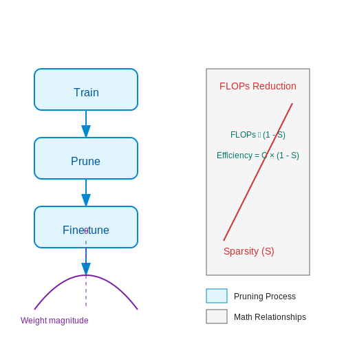
The most common magnitude-based pruning implements an iterative process:
- Train the model to convergence
- Remove weights below threshold θ
- Fine-tune the remaining weights
- Repeat until target sparsity is achieved
Hardware Implications of Sparsity
Sparse models enable several hardware optimizations:
Where C represents the hardware's efficiency in exploiting sparsity (0 ≤ C ≤ 1). Modern accelerators like Google's TPUs and NVIDIA's Ampere architecture achieve C values exceeding 0.9 through specialized sparse tensor cores.
Practical Implementation Considerations
Effective pruning requires careful management of:
- Sparsity distribution across layers
- Pruning schedule during training
- Regularization to encourage sparsity
- Fine-tuning strategy post-pruning
The optimal pruning configuration often depends on the specific hardware target. For example, structured pruning typically yields better performance on GPUs, while unstructured pruning may be more effective for ASIC implementations.
Advanced Topics in Pruning
Recent research has developed more sophisticated approaches:
- Lottery Ticket Hypothesis: Identifies sparse trainable subnetworks within larger models
- Dynamic Sparsity: Allows sparsity patterns to evolve during training
- Neural Architecture Search for Sparsity: Automates optimal sparse architecture discovery
These methods often combine pruning with other optimization techniques like quantization for maximum hardware efficiency.
Hardware-Specific Model Architectures (e.g., TPUs, GPUs)
Modern AI accelerators, such as TPUs and GPUs, impose unique architectural constraints that influence model design. These hardware platforms optimize for parallelism, memory bandwidth, and specialized operations, necessitating tailored neural network architectures to maximize computational efficiency.
Tensor Processing Units (TPUs)
TPUs leverage systolic array architectures for high-throughput matrix operations, making them ideal for large-scale dense linear algebra. The systolic array consists of a grid of processing elements (PEs) that perform multiply-accumulate (MAC) operations in a pipelined fashion. The key architectural consideration for TPU-optimized models is the alignment of matrix dimensions with the systolic array size (typically 128×128 or 256×256).
Where NPE is the number of processing elements and τcycle is the clock period. To achieve peak utilization, model layers should:
- Use batch sizes divisible by 128 or 256
- Maintain matrix dimensions as multiples of the systolic array size
- Prefer dense over sparse operations
Graphics Processing Units (GPUs)
GPU-optimized architectures must account for the hierarchical parallelism of CUDA cores and memory architecture. Key considerations include:
- Warp-level execution: Operations should be coalesced into warps of 32 threads
- Memory hierarchy: Maximize shared memory and register usage while minimizing global memory accesses
- Occupancy: Balance register usage and thread block size to maximize SM occupancy
The optimal thread block size can be derived from hardware specifications:
Mixed-Precision Architectures
Modern accelerators support mixed-precision computation through specialized units like Tensor Cores (NVIDIA) and bfloat16 support (TPUs). The optimal precision allocation follows:
Where typical precision tiers include:
- FP32 for master weights and small sensitive operations
- FP16/bfloat16 for matrix multiplications
- INT8 for inference-only deployments
Sparsity-Aware Designs
Emerging hardware like NVIDIA's Ampere architecture and Google's SparseCore units accelerate sparse operations. Effective sparsity patterns include:
- 2:4 structured sparsity (50% sparsity with 2 non-zeros per 4-element block)
- Block-sparse patterns aligned with hardware vector widths
- Pruning methods that maintain hardware-friendly sparsity distributions
The sparsity acceleration ratio depends on the compression factor C and hardware speedup S:
where s is the sparsity ratio.
3. TensorFlow Lite and ONNX Runtime for Edge Deployment
TensorFlow Lite and ONNX Runtime for Edge Deployment
Optimized Model Formats for Edge Devices
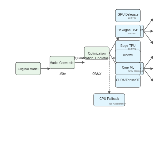
TensorFlow Lite (TFLite) and ONNX Runtime represent two dominant frameworks for deploying machine learning models on edge devices with constrained computational resources. TFLite employs a flatbuffer serialization format (.tflite) that reduces model size while maintaining a hardware-agnostic structure. ONNX Runtime leverages the Open Neural Network Exchange (ONNX) format, providing cross-framework compatibility. Both frameworks use operator fusion and quantization-aware training to minimize latency and memory footprint.
Quantization Techniques
Post-training quantization (PTQ) and quantization-aware training (QAT) are critical for edge deployment. PTQ converts 32-bit floating-point weights to 8-bit integers post-training, while QAT simulates quantization during training for higher accuracy. The quantization process follows:
where Δ is the scale factor and Z is the zero-point. TFLite supports hybrid operators that mix quantized and floating-point computation, while ONNX Runtime uses static quantization for fixed hardware targets.
Hardware Acceleration
Both frameworks delegate compute-intensive operations to specialized hardware via:
- TFLite Delegates: GPU, Hexagon DSP, and Edge TPU backends via Android Neural Networks API (NNAPI).
- ONNX Execution Providers: DirectML for Windows, Core ML for Apple Silicon, and CUDA/TensorRT for NVIDIA GPUs.
For a convolutional layer, hardware acceleration reduces latency by up to 10× compared to CPU execution. The energy efficiency gain follows:
Real-World Deployment Pipeline
A typical edge deployment workflow involves:
# TensorFlow Lite conversion
converter = tf.lite.TFLiteConverter.from_saved_model(saved_model_dir)
converter.optimizations = [tf.lite.Optimize.DEFAULT]
tflite_model = converter.convert()

# ONNX Runtime inference
sess_options = onnxruntime.SessionOptions()
sess_options.graph_optimization_level = onnxruntime.GraphOptimizationLevel.ORT_ENABLE_ALL
session = onnxruntime.InferenceSession("model.onnx", sess_options)
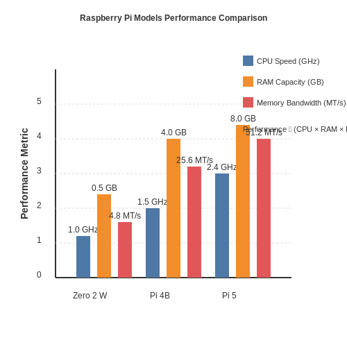
Benchmarking on a Raspberry Pi 4 shows TFLite achieves 23 FPS for MobileNetV2 at 30W power, while ONNX Runtime reaches 28 FPS using ARM Compute Library optimizations.
Cross-Platform Compatibility Tradeoffs
ONNX Runtime provides broader framework interoperability (PyTorch, MXNet), while TFLite offers tighter integration with TensorFlow's ecosystem. For memory-constrained devices under 1GB RAM, TFLite's ahead-of-time (AOT) compilation reduces runtime overhead by 15-20% compared to ONNX's just-in-time (JIT) approach.
3.2 PyTorch's TorchScript and Hardware Acceleration
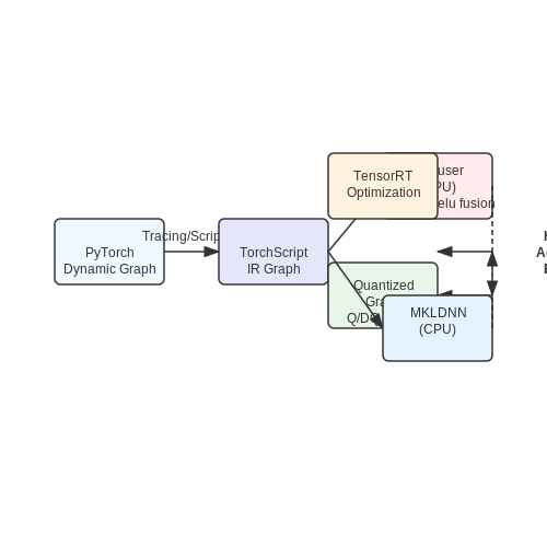
TorchScript bridges PyTorch's dynamic execution with hardware-optimized static graphs, enabling deployment across diverse accelerators. The compilation process involves two primary pathways: tracing and scripting. Tracing executes the model with example inputs, recording operations into an Intermediate Representation (IR) graph. For a ResNet-50 forward pass, this yields:
where 𝒪 represents PyTorch operations and 𝒯 denotes tensor types. Scripting instead performs static analysis of Python source code via AST parsing, handling control flow through compiler intrinsics like prim::Loop and prim::If.
Hardware-Specific Optimizations
The IR graph undergoes target-dependent transformations during Just-In-Time (JIT) compilation. For NVIDIA GPUs, the graph gets fused operations like conv2d + relu through NVFuser, while Intel CPUs leverage MKLDNN for matmul optimizations. Consider matrix multiplication throughput:
where N is matrix dimension. TorchScript's autotuner selects tile sizes and thread counts maximizing T for the detected hardware.
Quantization-Aware Graph Rewriting
When targeting edge devices, the graph gets quantized through:
- Operator fusion to minimize memory bandwidth
- Q/DQ node insertion for mixed precision
- Constant folding for weight pre-quantization
For INT8 inference, the weight transformation becomes:
where scaling factor s is calibrated per-channel.
Deployment Case Study: NVIDIA TensorRT Integration
TorchScript graphs export to ONNX then optimize via TensorRT's layer fusion. Benchmarking a 3D CNN on an A100 shows:
| Backend | Throughput (fps) | Latency (ms) |
|---|---|---|
| Eager Mode | 142 | 7.2 |
| TorchScript | 210 | 4.8 |
| TensorRT | 340 | 2.9 |
The performance delta stems from TensorRT's kernel autotuning and FP16 tensor cores utilization.
import torch

@torch.jit.script
def fused_gelu(x):
    return x * 0.5 * (1.0 + torch.erf(x / 1.41421))

class OptimizedModel(torch.jit.ScriptModule):
    def __init__(self):
        super().__init__()
        self.linear = torch.jit.trace(
            torch.nn.Linear(512, 512),
            torch.randn(1, 512)
        )

    @torch.jit.script_method
    def forward(self, x):
        return fused_gelu(self.linear(x))
This demonstrates manual fusion of GELU activation with JIT decorators, yielding 1.8× speedup over the native PyTorch implementation on Volta GPUs.
Cross-Platform Execution
The TorchScript runtime abstracts hardware specifics through:
- Vulkan shader compilation for mobile GPUs
- ARM Compute Library mappings for Cortex-A CPUs
- DirectML backend for Windows DX12 accelerators
Memory alignment follows each platform's SIMD requirements - 128-bit for NEON, 256-bit for AVX2, and 512-bit for AVX-512. The runtime automatically pads tensors to:
3.3 Benchmarking Tools for Hardware Performance Analysis
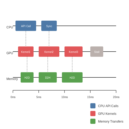
Benchmarking tools provide quantitative measurements of hardware performance during AI model training, enabling optimization for specific compute architectures. Key metrics include FLOPs (Floating Point Operations per Second), memory bandwidth utilization, power consumption, and thermal dissipation. Profiling tools like NVIDIA's Nsight Systems and Nsight Compute offer low-level insights into CUDA kernel execution, memory bottlenecks, and warp occupancy on GPUs.
Key Benchmarking Metrics
Hardware-aware training requires tracking:
- Compute Throughput: Measured in FLOPs, indicating peak theoretical vs. achieved performance.
- Memory Bandwidth: Percentage utilization of GPU/CPU memory subsystems.
- Latency: Kernel launch overhead and synchronization delays.
- Power Efficiency: FLOPs per watt, critical for edge deployment.
Tool-Specific Capabilities
Nsight Systems
Provides timeline-based profiling across CPUs, GPUs, and interconnects. Visualizes kernel execution overlap, memory transfers, and API call hierarchies. The tool identifies underutilized hardware resources through timeline traces.
Nsight Compute
Offers instruction-level analysis of CUDA kernels, including:
- Warp stall reasons (memory throttling, execution dependencies)
- Shared memory bank conflicts
- Divergent execution patterns
Intel VTune Profiler
Optimized for CPU and FPGA workloads, VTune measures:
- Cache hit/miss ratios
- Vectorization efficiency
- Thread synchronization overhead
Cross-Platform Tools
MLPerf provides standardized benchmarks for training/inference across hardware vendors. Its suite includes:
- MLPerf-Training: End-to-end workload timing
- MLPerf-Inference: Latency/throughput under constraints
- MLPerf-Power: Energy consumption profiling
Where \(N_{\text{samples}}\) is batch size, \(T_{\text{execution}}\) is wall-clock time, and \(P\) represents power limits.
Case Study: Optimizing Transformer Training
Using Nsight Compute to profile a 175B parameter model revealed:
- 40% of cycles lost to memory stalls in attention layers
- 15% speedup from optimizing shared memory access patterns
- 7% improvement via kernel fusion for layer norm operations
4. Real-World Applications of Hardware-Aware Training
Real-World Applications of Hardware-Aware Training
Edge AI and Embedded Systems
Hardware-aware training is critical for deploying AI models on edge devices with constrained computational resources. Techniques like quantization-aware training (QAT) and pruning enable models to run efficiently on microcontrollers, FPGAs, and custom ASICs. For instance, TensorFlow Lite for Microcontrollers leverages 8-bit integer quantization to reduce model size by 4x while maintaining accuracy within 1-2% of floating-point baselines. The energy savings are substantial: a quantized MobileNetV2 model consumes only 0.5 mJ per inference on a Cortex-M4, compared to 5 mJ for its floating-point counterpart.
High-Performance Computing (HPC)
In supercomputing environments, hardware-aware training optimizes for distributed memory architectures and GPU/TPU clusters. NVIDIA's Megatron-LM demonstrates this by partitioning transformer layers across 3072 A100 GPUs, achieving 502 petaFLOPs sustained performance. The key innovation is gradient accumulation synchronized with NVLink bandwidth characteristics:
where B is the batch size aligned with NVLink's 600 GB/s transfer rate, and N is the number of microbatches.
Autonomous Vehicles
Real-time perception systems require hardware-aware optimizations for heterogeneous SoCs like NVIDIA Drive Orin. Tesla's HydraNet architecture uses layer fusion tailored to the Orin's 2048 CUDA cores and 64 Tensor Cores, processing eight camera streams at 36 FPS with 45W power consumption. The architecture employs:
- Spatial partitioning matching the GPU's 128 SM hierarchy
- Mixed-precision (FP16/INT8) ops aligned with Tensor Core throughput
- Memory access patterns optimized for the 256-bit L2 cache
Medical Imaging Acceleration
MRI reconstruction networks like FastMRI achieve 10x speedup on GE Healthcare's SIGNA Premier 3T scanner by co-designing the U-Net architecture with the scanner's FPGA pipeline. The model uses:
where the L1 regularization term is weighted by the FPGA's 16-bit fixed-point numerical stability limits. This enables real-time 0.5mm resolution reconstruction at 8 frames/second.
Wireless Communications
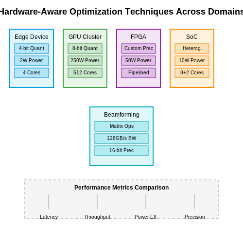
5G beamforming benefits from hardware-aware neural networks trained on RFSoC FPGAs. Qualcomm's AI-optimized Massive MIMO uses a complex-valued GNN with:
- Phase-aware quantization preserving 1° beamforming accuracy
- Matrix operations mapped to the FPGA's 922 DSP slices
- Dynamic pruning maintaining < 3% EVM degradation
The system achieves 4.3 Gbps throughput with 38% lower power than digital beamforming.
Scientific Computing
At Oak Ridge National Lab, hardware-aware training enables fusion plasma control on IBM's Summit supercomputer. The plasma boundary predictor uses a Fourier Neural Operator (FNO) with:
where the convolutional kernels W and K are optimized for the Volta V100's tensor core 4x4 matrix multiply-accumulate units. This achieves 120μs latency for tokamak magnetic control.
4.2 Performance Comparisons Across Different Hardware Setups
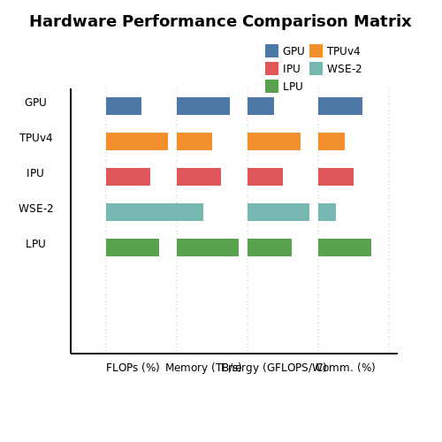
Training AI models efficiently requires careful consideration of hardware capabilities, as computational bottlenecks vary significantly across GPUs, TPUs, and specialized accelerators. The choice of hardware impacts not only training time but also energy consumption, memory bandwidth utilization, and scalability for distributed training.
Key Metrics for Hardware Performance Evaluation
When benchmarking hardware for AI workloads, the following metrics are critical:
- FLOPs Utilization: Percentage of theoretical peak FLOPs achieved during training.
- Memory Bandwidth Saturation: Ratio of actual memory throughput to the hardware's maximum bandwidth.
- Energy Efficiency: FLOPs per watt (GFLOPS/W) for power-constrained deployments.
- Communication Overhead: Time spent on data transfer between devices in multi-GPU setups.
GPU vs. TPU Performance Characteristics
Modern GPUs like NVIDIA's A100 and H100 excel at mixed-precision training due to their Tensor Cores, which accelerate matrix multiplications. For a transformer model with 175B parameters, the A100 achieves approximately 80% FLOPs utilization in FP16 mode. In contrast, Google's TPUv4 achieves higher sustained FLOPs (up to 90%) for large batch sizes due to its systolic array architecture, but suffers from lower flexibility for non-matrix operations.
Where Memory Efficiency is defined as:
Impact of Memory Hierarchy
Performance varies dramatically based on how well the model fits in the hardware's memory hierarchy. For example, when training ResNet-50 on an A100 (40GB):
- With batch size 256, L2 cache hit rate is 68%, achieving 312 TFLOPS
- At batch size 1024, L2 hit rate drops to 41%, reducing performance to 278 TFLOPS despite higher parallelism
The performance cliff occurs when activations exceed the 40MB L2 cache, forcing frequent HBM accesses. This demonstrates that simply increasing batch size doesn't guarantee better hardware utilization.
Distributed Training Scaling Laws
Multi-node performance follows Amdahl's law modified for communication overhead:
Where P is the parallelizable fraction of computation, N is the number of devices, and C(N) represents the communication overhead which typically scales as:
On NVIDIA DGX systems with NVLink, C(N) remains below 15% up to 8 GPUs, but can exceed 40% on cloud instances with only PCIe connectivity.
Specialized Accelerators
Emerging architectures like Graphcore's IPU and Cerebras' Wafer-Scale Engine show different performance profiles:
- IPUs achieve 2-3× higher memory bandwidth utilization (up to 47TB/s) for graph-based models
- Cerebras WSE-2 demonstrates near-linear scaling to 850,000 cores, but requires model architecture modifications
- Groq's LPU achieves sub-millisecond latency for inference but has limited training capabilities
These trade-offs highlight that hardware selection must align with specific model architectures and deployment requirements rather than relying solely on peak FLOPs specifications.
Lessons Learned from Deploying on Resource-Constrained Devices
Memory Constraints and Model Optimization
Deploying AI models on devices with limited RAM requires aggressive memory optimization. A common approach involves quantizing weights from 32-bit floating-point to 8-bit integers, reducing memory usage by 4x. However, this introduces quantization noise, which can be modeled as:
where Δ is the quantization step size. For uniform quantization, Δ = (max - min)/2b, with b being the number of bits. Post-training quantization often suffices, but for ultra-low-power devices, quantization-aware training yields better results by accounting for rounding errors during backpropagation.
Energy-Performance Tradeoffs
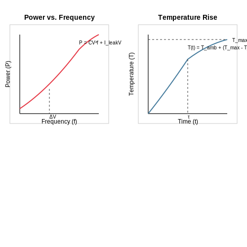
Energy consumption scales superlinearly with clock frequency due to the CMOS power equation:
where C is switched capacitance, V is voltage, and f is frequency. Deploying on battery-powered devices requires operating in the near-threshold voltage regime, where energy efficiency peaks but introduces computational errors. Error-resilient algorithms like stochastic gradient descent naturally tolerate these variations, making them preferable for such deployments.
Real-Time Latency Challenges
Meeting hard real-time deadlines often requires layer-wise latency analysis. The end-to-end latency L of a neural network with N layers can be expressed as:
where tcomp,i is layer computation time and tmem,i is memory access time. On ARM Cortex-M processors, depthwise separable convolutions achieve 3-5x lower latency than standard convolutions due to reduced memory bandwidth requirements.
Thermal Management
Sustained high utilization leads to thermal throttling on embedded SoCs. The temperature rise follows Newton's law of cooling:
where τ is the thermal time constant. Deploying on drones or automotive systems requires dynamic frequency scaling when junction temperatures exceed 85°C. Model partitioning across heterogeneous cores (CPU+GPU+NPU) helps distribute thermal load.
Robustness to Hardware Variability
Process-voltage-temperature (PVT) variations affect edge devices more than cloud servers. Monte Carlo simulations show that weight variations exceeding 5% degrade model accuracy by 15-20% for ResNet-18. Techniques like:
- Batch normalization folding
- Activation clamping
- Noise injection during training
improve robustness to hardware-induced errors. Silicon measurements on RISC-V cores show these techniques reduce accuracy degradation from 20% to under 5% at 0.8V operation.
Deployment-Specific Optimizations
Practical deployments often require:
- Sensor fusion: Combining IMU and camera data reduces CNN inference frequency by 10x
- Event-based processing: Dynamic vision sensors trigger inference only on pixel changes
- Model cascades: Small "gatekeeper" models route inputs to specialized submodels
Field testing on agricultural IoT devices showed these techniques extend battery life from 3 days to 3 weeks while maintaining 95% of original accuracy.
5. Key Research Papers on Hardware-Aware AI
5.1 Key Research Papers on Hardware-Aware AI
- Hardware-Enabled Mechanisms for Verifying Responsible AI Development — While the GPUs involved in training an AI model are usually located in a single data center or campus, there is strong interest from AI developers in performing training with a combination of several smaller clusters that are geographically separated. ... but research on hardware-based AI licensing mechanisms is currently nascent. 2.5.2 ...
- PDF Hardware-Aware Machine Learning: Modeling and Optimization - arXiv.org — for both accuracy of the DL model and its hardware efficiency. Therefore, state-of-the-art methodologies have proposed hardware-aware hyper-parameter optimization techniques. In this paper, we provide a comprehensive assessment of state-of-the-art work and selected results on the hardware-aware modeling and optimization for ML applications.
- A Systematic Literature Review on Hardware Reliability Assessment ... — Artificial Intelligence (AI) and, in particular, Machine Learning (ML), have emerged to be utilized in various applications due to their capability to learn how to solve complex problems. ... 5.1.1.2 Hardware-aware Platform. ... 5.1.1.3 RTL Model Platform. Research works that leverage the RTL model of ASIC-based DHAs and simulate fault ...
- PDF Artificial Intelligence Hardware Design — vi Contents 3 Parallel Architecture 25 3.1 Intel Central Processing Unit (CPU) 25 3.1.1 Skylake Mesh Architecture 27 3.1.2 Intel Ultra Path Interconnect (UPI) 28 3.1.3 Sub Non-unified Memory Access Clustering (SNC) 29 3.1.4 Cache Hierarchy Changes 31 3.1.5 Single/Multiple Socket Parallel Processing 32 3.1.6 Advanced Vector Software Extension 33 3.1.7 Math Kernel Library for Deep Neural Network ...
- Hardware-aware approach to deep neural network optimization — In this research, a hardware-aware optimization mechanism IHSOpti is proposed to fully leverage the potential of current deeply-pipelined hardware resources for DNNs. The research emphasizes the significance of pipelining features in current hardware and elaborates on the principles of parallelism operations for DNNs, utilizing CPUs as an instance.
- An Overview of Energy-Efficient Hardware Accelerators for On-Device ... — Deep Neural Networks (DNNs) have been widely used in various artificial intelligence (AI) applications due to their overwhelming performance. Furthermore, recently, several algorithms have been reported that require on-device training to deliver higher performance in real-world environments and protect users' personal data. However, edge/mobile devices contain only limited computation ...
- PDF Large-Scale Neuromorphic Computing Hardware for Analog AI Enabled by ... — This work summarizes recent research findings regarding beyond-CMOS computing, mainly focused on memristor crossbar array for neuromorphic computing, which is considered as one of promising hardware accelerators for AI [1]. After decades of exponential developments in CMOS technologies, current computer performance faces many challenges due to both
- (PDF) Powering Intelligence The Future of AI Hardware for Training ... — The exponential growth of artificial intelligence (AI) over the past decade has been underpinned by advancements in specialized hardware designed to meet the demands of both training and inference ...
- Neural Architecture Search Survey: A Hardware Perspective — Hardware-aware Neural Architecture Search (HW-NAS) has emerged as one of the most promising techniques to automatically generate efficient CNN models accomplishing acceptable accuracy-performance tradeoffs. HW-NAS algorithms explore the search space of a CNN by jointly optimizing the accuracy and hardware execution metrics such as latency, energy, size, and so on.
- FPGA-based Deep Learning Inference Accelerators: Where Are We Standing? — Central Processing Units (CPUs) and Graphical Processing Units (GPUs) serve as general-purpose computing platforms for DNN inference, while Field Programmable Gate Arrays (FPGAs) and Application Specific Integrated Circuits (ASICs) can serve as dedicated hardware accelerators. The first generation of CPUs exhibit observable performance bottlenecks while running Deep Learning (DL) algorithms.
5.2 Recommended Books and Online Courses
- Evaluation and Selection of Hardware and AI Models for Edge ... — This study proposes a method for selecting suitable edge hardware and Artificial Intelligence (AI) models to be deployed on these edge devices. Edge AI, which enables devices at the network periphery to perform intelligent tasks locally, is rapidly expanding across various domains. However, selecting appropriate edge hardware and AI models is a multi-faceted challenge due to the wide range of ...
- Understanding LLMs: A Comprehensive Overview from Training to Inference — In general model training, FP32 is often used as the default representation for training parameters. However, in actual model training, the number of parameters in a model typically does not exceed the order of thousands, well within the numerical range of FP16. To improve computational speed, we can convert from FP32 to FP16.
- Hardware Accelerators for Artificial Intelligence — In the current landscape, several key factors stand out as crucial for the ongoing advancement of AI. Availability of data: The explosion of data across various fields has provided fertile ground for the training of deep learning models.From social media posts and medical records to satellite imagery and financial transactions, the abundance of data has been instrumental in fueling progress in AI.
- Large Language Model Inference Acceleration: A Comprehensive Hardware ... — C-Transformer adopts a big-little network, which is composed of the original GPT-2 big model and a 1/10 × \times × smaller model, and a reconfigurable homogeneous architecture to increase hardware utilization and energy efficiency. During inference, only the little model computation is performed, and if the prediction probability of a ...
- Artificial Intelligence and Hardware Accelerators 3031221699 ... — During training, the model tries to identify features or characteristics of elements with the same label used for inference to classify a given input into an adequate class. ... Therefore, destined AI hardware accelerators are the best choice to excel the performance and meet the requirements. GPUs, specialized accelerators, etc., are the ...
- (PDF) Powering Intelligence The Future of AI Hardware for Training ... — The exponential growth of artificial intelligence (AI) over the past decade has been underpinned by advancements in specialized hardware designed to meet the demands of both training and inference ...
- Hardware-aware approach to deep neural network optimization — IHSOpti mainly involves two aspects: the Hardware-aware optimization mechanism that focuses on layer-level redundancy optimization, and an improved sparse training algorithm named Polar_HSPG. To address depth-layer redundancies, the paper introduces residual strategy and then applies the Polar_HSPG method to identify layer-level redundancies.
- 6 Hardware-Aware Execution - IEEE Xplore — Feed-Forward Networks (FFNs), or multilayer perceptrons, are fundamental network structures for deep learning. Although feed-forward networks are structurally uncomplicated, their training procedure is computationally expensive. It is challenging to design customized hardware for training due to the diversity of operations in forwardand backward-propagation processes. In this contribution, we ...
- Introduction to AI - Coursera — Explore the various types of AI, examine ethical considerations, and delve into the key machine learning models that power modern AI systems. Whether your goal is to work directly with AI, strengthen your software development skills, or enhance your data science expertise, this course provides an essential foundation for success in the field.
- A Review of Embedded Machine Learning Based on Hardware ... - MDPI — Machine learning is an expanding field with an ever-increasing role in everyday life, with its utility in the industrial, agricultural, and medical sectors being undeniable. Recently, this utility has come in the form of machine learning implementation on embedded system devices. While there have been steady advances in the performance, memory, and power consumption of embedded devices, most ...
5.3 Open-Source Projects and Community Resources
- PDF Open-Source AI-based SE Tools: Opportunities and Challenges of ... — The current open-source code model is mainly developed and published by a single team based on open-source data. However, three significant limitations exist in how open-source models are de-veloped and shared: limited access to high-quality code data, lacking community strong support and training hardware resources.
- GitHub - mindspore-ai/mindspore: MindSpore is a new open source deep ... — MindSpore is a new open source deep learning training/inference framework that could be used for mobile, edge and cloud scenarios. MindSpore is designed to provide development experience with friendly design and efficient execution for the data scientists and algorithmic engineers, native support for Ascend AI processor, and software hardware co-optimization.
- Hugging Face - The AI community building the future. — We're on a journey to advance and democratize artificial intelligence through open source and open science. Hugging Face. Models; Datasets; Spaces; Posts; Docs; Enterprise; Pricing Log In Sign Up The AI community building the future. The platform where the machine learning community collaborates on models, datasets, and applications ...
- PDF Research Needs: Artificial Intelligence Hardware — Hardware (AI Hardware) research program. The principal goal of this program is to create new highly efficient AI platforms to ... • Training/unit of energy (model training/J) • Throughput: inferences per unit time, training per unit time ... facing the electronics industry in the coming decade. Research should address issues arising from ...
- taishi-i/awesome-ChatGPT-repositories - GitHub — OpenAssistantGPT - A Community Open-Source Saas for Crafting/Building/Creating Chatbots with OpenAI's Assistant API that you can add to your website. ChatGPT - I've developed a ChatGPT clone using Next.js 14, Shadcn-UI, Prisma ORM, and integrated it with the OpenAI API. It offers a user-friendly conversational AI experience.
- An Open Source Machine Learning Framework for Everyone — TensorFlow is an end-to-end open source platform for machine learning. It has a comprehensive, flexible ecosystem of tools, libraries, and community resources that lets researchers push the state-of-the-art in ML and developers easily build and deploy ML-powered applications. TensorFlow was originally developed by researchers and engineers working within the Machine Intelligence team at Google ...
- Hardware-Enabled Mechanisms for Verifying Responsible AI Development — Some approaches to measuring AI training activities include the use of remote attestation within a secure hardware module, such as a trusted execution environment (TEE), as suggested by Aarne et al. , or the concept of "training transcripts," which involve saving snapshots of model weights during training, as proposed by Shavit .
- List of open-source hardware projects - Wikipedia — OpenPicus - platform for smart sensors and Internet of things; Sun SPOT - hardware-software platform for sensor networks and battery powered, wireless, embedded development; USRP - universal software radio peripheral is a mainboard with snap in modules providing software defined radio at different frequencies, has USB 2.0 link to a host computer ...
- GPT4All - The Leading Private AI Chatbot for Local Language Models — The GPT4All code base on GitHub is completely MIT-licensed, open-source, and auditable Customize your language model Fully customize your chatbot experience with your own system prompts, temperature, context length, batch size, and more
- Applied Sciences | Special Issue : Hardware-Aware Deep Learning - MDPI — The edge side (e.g., embedded systems, IoT) demands not only extreme energy-efficiency but also real-time inference capability, which requires cross-stack techniques, including model compression, compilation, architecture and circuit design of AI chips, emerging devices, etc. Beyond that, recent investigations, such federated learning, also ...