Vision Transformers (ViT) Explained
1. From CNNs to Transformers: The Evolution of Vision Models
From CNNs to Transformers: The Evolution of Vision Models
Convolutional Neural Networks (CNNs) dominated computer vision for nearly three decades, with architectures like LeNet, AlexNet, and ResNet establishing fundamental principles of hierarchical feature learning. The key innovation was the local receptive field, where filters slide across spatial dimensions to capture translation-invariant patterns through shared weights. For an input image I ∈ ℝH×W×C, a CNN applies discrete convolution operations:
where K ∈ ℝkh×kw×C represents the learnable kernel. This inductive bias enabled efficient processing of grid-structured data but introduced limitations:
- Fixed receptive fields struggle with long-range dependencies
- Pooling operations discard positional information
- Hierarchical reduction loses fine-grained details
The Attention Paradigm Shift
Transformers, introduced in natural language processing, demonstrated that self-attention mechanisms could model arbitrary dependencies without convolutional constraints. The scaled dot-product attention computes:
where queries Q, keys K, and values V are learned projections. Vision Transformers (ViT) adapt this by splitting images into N non-overlapping patches {xp}i=1N, treating each as a token:
with patch embedding matrix E and positional encoding Epos. The transformer encoder layers then apply:
where MSA is multi-head self-attention and LN denotes layer normalization.
Hybrid Architectures and Efficiency
Transitional architectures like DeiT and ConvMixer blended CNN inductive biases with transformer flexibility. The convolutional stem in hybrid models processes early visual features more efficiently, while axial attention reduces the quadratic complexity of full self-attention from O(N2) to O(N√N).
Modern variants like Swin Transformers reintroduce hierarchical processing through shifted windows, while Perceiver IO handles multimodal inputs through latent space projections. The evolution reflects a fundamental tradeoff: CNNs offer computational efficiency for local patterns, while transformers provide flexible relational modeling at greater memory cost.

Core Principles of Transformer Architecture
Self-Attention Mechanism
The self-attention mechanism is the cornerstone of transformer architectures, enabling the model to weigh the importance of different input tokens dynamically. Given an input sequence X ∈ ℝn×d, where n is the sequence length and d is the embedding dimension, self-attention computes three matrices: queries (Q), keys (K), and values (V):
where WQ, WK, WV ∈ ℝd×dk are learnable weight matrices. The attention scores are computed as:
The scaling factor √dk prevents gradient saturation in the softmax function. Multi-head attention extends this by applying h parallel attention heads, concatenating their outputs:
Positional Encoding
Since transformers lack recurrent or convolutional operations, positional encodings inject sequential order information. For a position pos and dimension i, the encoding uses sinusoidal functions:
This choice allows the model to generalize to unseen sequence lengths better than learned positional embeddings.
Layer Normalization and Residual Connections
Transformers employ residual connections followed by layer normalization (LN) around each sub-layer (attention and feed-forward networks). For a sub-layer function F and input x:
This architecture mitigates vanishing gradients and accelerates convergence. The feed-forward network (FFN) consists of two linear transformations with a ReLU activation:
Vision Transformer Adaptations
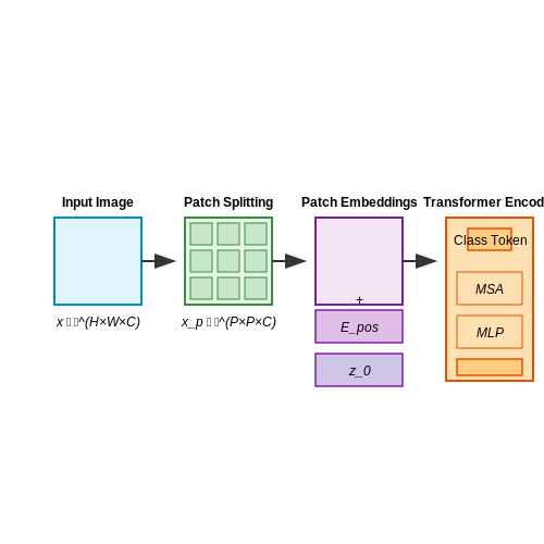
In Vision Transformers (ViT), images are split into non-overlapping patches xp ∈ ℝN×(P²·C), where P is patch size and C is channels. These are linearly projected into patch embeddings:
where E ∈ ℝ(P²·C)×D is the patch embedding matrix and Epos ∈ ℝ(N+1)×D are positional embeddings. A learnable [class] token prepended to the sequence aggregates global information.

1.3 Key Innovations in Vision Transformers
Patch Embeddings and Linear Projections
Unlike convolutional networks, Vision Transformers (ViT) process images by dividing them into fixed-size non-overlapping patches, typically 16×16 pixels. Each patch is flattened into a vector xp ∈ ℝ(P²·C), where P is the patch size and C is the number of channels. A trainable linear projection E maps these patches into a D-dimensional embedding space:
Here, E ∈ ℝ(P²·C)×D is the embedding matrix, Epos ∈ ℝ(N+1)×D adds positional information, and xclass is a learnable classification token inspired by BERT.
Multi-Head Self-Attention (MHSA) in ViT
ViT leverages scaled dot-product attention, where queries (Q), keys (K), and values (V) are computed via learned projections. For h attention heads, the output is:
MHSA concatenates outputs from all heads and projects them back to dimension D:
where WO ∈ ℝD×D. This allows the model to jointly attend to information from different representation subspaces.
Hybrid Architectures and CNN-ViT Fusion
Hybrid ViTs replace raw patch embeddings with feature maps from CNNs. Let F be a CNN generating a feature map of size H'×W'×C'. The patches are then:
This leverages CNNs' local feature extraction while preserving ViT's global receptive field. Models like DeiT and Swin Transformer further optimize this interplay.
Efficient Attention Mechanisms
To address ViT's quadratic complexity (O(N²)), innovations include:
- Windowed Attention: Restricts attention to local windows (e.g., Swin Transformer).
- Axial Attention: Decomposes 2D attention into row-wise and column-wise operations.
- Performer Kernels: Approximates softmax attention using orthogonal random features.
Positional Encoding Variants
ViT abandons convolutional inductive bias, making positional encoding critical. Alternatives to standard fixed sine/cosine embeddings include:
- Relative Position Bias: Adds learnable biases to attention scores based on patch distances.
- Rotary Position Embedding (RoPE): Encodes position via rotation matrices in query/key vectors.

2. Patch Embedding: Converting Images into Sequences
Patch Embedding: Converting Images into Sequences
Traditional convolutional neural networks (CNNs) process images through hierarchical local operations, but Vision Transformers (ViTs) treat images as sequences of patches, leveraging self-attention mechanisms. The first critical step in ViTs is patch embedding, which decomposes an input image into non-overlapping patches and projects them into a lower-dimensional space.
Image Partitioning into Patches
Given an input image I ∈ ℝH×W×C (height H, width W, channels C), it is divided into N non-overlapping patches of size P×P. The number of patches N is computed as:
Each patch xp ∈ ℝP×P×C is flattened into a vector of dimension P2C. For example, a 224×224 RGB image split into 16×16 patches yields N = 196 patches, each represented as a 768-dimensional vector (16×16×3).
Linear Projection to Embedding Space
The flattened patches are mapped to a D-dimensional embedding space via a trainable linear projection E ∈ ℝ(P²C)×D:
where ep is a positional embedding added to retain spatial information. The projection matrix E is learned during training, enabling the model to adaptively weight patch features.
Positional Embeddings
Since transformers are permutation-invariant, positional embeddings epos ∈ ℝN×D are added to the patch embeddings to encode spatial relationships. Two common approaches are:
- Learned positional embeddings: Treated as trainable parameters optimized during training.
- Sinusoidal embeddings: Fixed embeddings using sine and cosine functions of varying frequencies.
The final input sequence to the transformer encoder is:
where zcls is an optional class token used for classification tasks.
Practical Implementation
In PyTorch, patch embedding can be implemented efficiently using a convolutional layer with kernel size and stride equal to P:
import torch.nn as nn

class PatchEmbedding(nn.Module):
    def __init__(self, img_size=224, patch_size=16, in_chans=3, embed_dim=768):
        super().__init__()
        self.proj = nn.Conv2d(in_chans, embed_dim,
                              kernel_size=patch_size,
                              stride=patch_size)

    def forward(self, x):
        x = self.proj(x)  # (B, D, H/P, W/P)
        x = x.flatten(2)  # (B, D, N)
        x = x.transpose(1, 2)  # (B, N, D)
        return x
Dimensionality Considerations
The choice of P and D involves trade-offs:
- Smaller patches (P = 8–12) capture finer details but increase computational cost (N ∝ 1/P2).
- Larger D improves representational capacity but raises memory usage quadratically in self-attention layers.
Hybrid architectures combine CNN feature maps with patch embeddings to balance locality and global context.

Positional Encodings for Spatial Information
Transformers, originally designed for sequential data, lack inherent spatial awareness. Vision Transformers (ViT) address this by incorporating positional encodings to preserve the spatial structure of image patches. Unlike convolutional networks, which implicitly capture locality through kernels, ViTs rely on explicit positional information to understand patch relationships.
Mathematical Formulation of Positional Encodings
The standard sinusoidal positional encoding used in NLP is adapted for 2D images. Given an image split into N × N patches, each patch at position (i, j) is assigned a positional embedding Pi,j ∈ ℝd, where d is the embedding dimension. The encoding for each dimension k is computed as:
These sinusoidal functions ensure that the model can generalize to unseen positions by encoding relative distances through phase shifts.
Learned vs. Fixed Positional Encodings
ViTs can use either fixed sinusoidal encodings or learned positional embeddings:
- Fixed encodings leverage predefined sinusoidal patterns, offering consistent inductive biases but no adaptability.
- Learned embeddings treat positional encodings as trainable parameters, allowing the model to optimize spatial relationships during training. Empirical results often favor learned embeddings for vision tasks due to their flexibility.
Relative Positional Encodings
Recent variants, such as Relative Positional Encodings (RPE), encode pairwise patch distances instead of absolute positions. For patches at (i, j) and (m, n), the relative offset (Δi, Δj) = (i−m, j−n) is mapped to an embedding:
where Wpos is a learnable matrix, and o is an offset to handle negative indices. RPEs improve translation invariance and reduce memory overhead for high-resolution images.
Practical Considerations
Positional encodings must handle variable input resolutions. Common strategies include:
- Interpolation: Resizing learned embeddings for new resolutions using bicubic or linear interpolation.
- Conditional position encodings: Dynamically generating embeddings based on patch content, as in CPVT.
In practice, the choice of encoding impacts model performance on tasks requiring fine-grained spatial understanding, such as object detection or semantic segmentation.

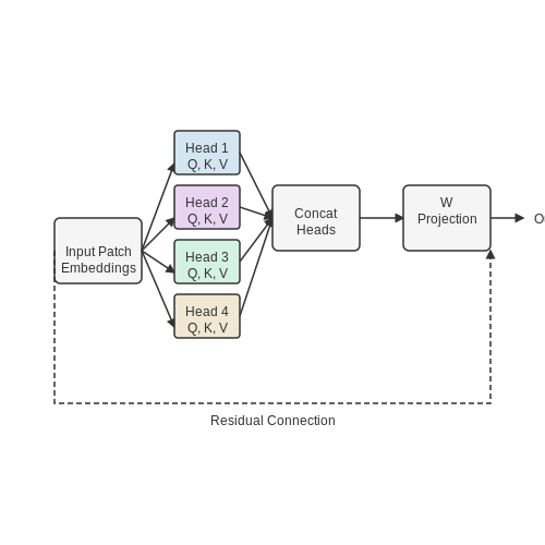
Multi-Head Self-Attention in ViT
Multi-head self-attention (MHSA) is the core mechanism enabling Vision Transformers (ViT) to model long-range dependencies across image patches. Unlike convolutional operations, which process local receptive fields, MHSA computes pairwise interactions between all patches, dynamically weighting their contributions based on relevance. This section derives the mathematical formulation of MHSA and explains its implementation in ViT.
Scaled Dot-Product Attention
The foundation of MHSA is scaled dot-product attention, which operates on three learned matrices: queries (Q), keys (K), and values (V). For an input sequence of N patches, each represented as a d-dimensional vector, the attention weights are computed as:
Here, dk is the dimension of the key vectors. The scaling factor 1/√dk prevents the dot products from growing too large in magnitude, which would push the softmax into regions of extremely small gradients.
Multi-Head Mechanism
MHSA extends this by employing h parallel attention heads, each with its own set of learned projections:
where WiQ ∈ ℝd×dk, WiK ∈ ℝd×dk, and WiV ∈ ℝd×dv are projection matrices for the i-th head. The outputs of all heads are concatenated and linearly transformed:
with WO ∈ ℝhdv×d. This allows the model to jointly attend to information from different representation subspaces.
Implementation in ViT
In ViT, MHSA operates on the sequence of patch embeddings. For an input image divided into N patches of size P×P, each patch is flattened and linearly projected to a d-dimensional space. The MHSA layer then computes:
where X is the input patch embeddings, and LayerNorm denotes layer normalization. The residual connection (X + MHSA(X)) stabilizes training by preserving gradient flow.
Computational Complexity
MHSA has a quadratic complexity O(N2d) due to the pairwise attention computation. For high-resolution images, this can be mitigated through techniques like windowed attention or linear attention approximations.
Practical Considerations
- Head Dimension: Typical configurations use dk = dv = d/h, balancing expressiveness and computational cost.
- Relative Position Bias: ViT often adds learnable position biases to the attention scores to encode spatial relationships.
- Efficiency: Memory usage can be optimized via flash attention or tiling strategies for large N.
The Role of MLP Layers and Layer Normalization
Vision Transformers (ViTs) rely on Multi-Layer Perceptrons (MLPs) and Layer Normalization (LayerNorm) to stabilize training and enhance feature transformation. The MLP block in a ViT consists of two linear layers separated by a Gaussian Error Linear Unit (GELU) activation, while LayerNorm ensures stable gradient flow by normalizing activations across the feature dimension.
MLP Layers in Vision Transformers
The MLP block processes each token independently, applying a non-linear transformation to the embedded features. Given an input x ∈ ℝd, the MLP operation is defined as:
where W1 ∈ ℝd×4d and W2 ∈ ℝ4d×d are learnable weights, and b1, b2 are biases. The expansion factor of 4 (d → 4d) increases model capacity while maintaining computational efficiency.
GELU Activation Function
The GELU activation introduces smooth non-linearity, approximating the expected value of a stochastic gate:
where Φ(x) is the standard Gaussian cumulative distribution function. This contrasts with ReLU's hard thresholding, allowing gradients to flow for negative inputs with non-zero probability.
Layer Normalization in ViTs
LayerNorm is applied before both the attention and MLP blocks, normalizing activations along the feature dimension:
where μ and σ are the mean and standard deviation computed across features, while γ and β are learnable affine parameters. This differs from BatchNorm by operating on individual samples rather than batch statistics, making it suitable for variable-length sequences.
Pre-Norm vs. Post-Norm Architectures
ViTs typically employ pre-norm configuration (LayerNorm before sub-layers), which empirically demonstrates better training stability than post-norm alternatives. The gradient flow through a pre-norm residual block can be expressed as:
where the identity term ensures direct gradient propagation even when the Jacobian of the transformation f becomes small.
Practical Implications
- Feature Mixing: MLPs enable cross-channel communication after attention-based token mixing.
- Training Stability: LayerNorm prevents exploding activations in deep architectures.
- Scalability: The 4d hidden dimension provides sufficient model capacity without quadratic attention cost.

3. Data Requirements and Preprocessing for ViT
3.1 Data Requirements and Preprocessing for ViT
Input Data Structure for Vision Transformers
Vision Transformers (ViT) process input images differently from convolutional neural networks (CNNs). Instead of sliding filters across spatial dimensions, ViTs treat images as sequences of flattened patches. Given an input image I ∈ ℝH×W×C (height H, width W, channels C), it is divided into N non-overlapping patches of size P×P:
Each patch xp ∈ ℝP²×C is linearly projected into D-dimensional embedding space using a trainable matrix E ∈ ℝ(P²·C)×D. A [CLS] token (xcls ∈ ℝD) prepends the sequence for classification tasks.
Patch Embedding and Positional Encoding
The patch embedding process combines linear projection with positional information:
where Epos ∈ ℝ(N+1)×D contains learnable positional embeddings. Unlike CNNs, ViTs have no inherent spatial inductive bias—positional encoding is crucial for modeling spatial relationships.
Normalization and Augmentation Strategies
ViTs require careful normalization due to their sensitivity to input scale:
- Per-patch normalization: Each patch is normalized independently using mean and variance computed across its spatial dimensions
- Global contrast normalization: Scales pixel values to zero mean and unit variance across the entire image
- Augmentations: MixUp (α=0.8), RandAugment (magnitude=9), and random erasing (probability=0.25) significantly improve performance
Large-Scale Pretraining Requirements
ViTs exhibit different scaling laws compared to CNNs:
| Model Variant | Minimum Pretraining Data | Optimal Resolution |
|---|---|---|
| ViT-B/16 | 14M images (JFT-300M) | 384×384 |
| ViT-L/32 | 100M+ images | 512×512 |
The data efficiency gap versus CNNs diminishes when pretraining exceeds 100M images. For smaller datasets (<1M images), hybrid architectures combining CNN feature extraction with Transformer blocks often outperform pure ViTs.
Computational Considerations
The quadratic complexity of self-attention imposes practical constraints:
Where N is the sequence length (number of patches). Strategies to manage computational cost include:
- Progressive resizing during training (start with 224×224, finetune at higher resolution)
- Mixed-precision training (FP16/FP32)
- Gradient checkpointing for memory optimization

3.2 Loss Functions and Optimization Strategies
Vision Transformers typically employ cross-entropy loss for classification tasks, formulated as:
where C is the number of classes, yi the ground truth label (one-hot encoded), and pi the predicted probability for class i. For regression tasks, mean squared error (MSE) loss is common:
Label Smoothing
To prevent overconfidence in predictions, label smoothing replaces hard 0/1 labels with smoothed values:
where α is the smoothing parameter (typically 0.1). This acts as a regularizer by encouraging the model to be less certain about its predictions.
Optimization Strategies
AdamW has emerged as the dominant optimizer for ViTs, combining adaptive momentum estimation with decoupled weight decay:
where η is the learning rate, λ the weight decay factor, and m̂t, v̂t are bias-corrected first and second moment estimates.
Learning Rate Scheduling
ViTs benefit from warmup schedules to stabilize early training. The linear warmup with cosine decay schedule is commonly used:
Advanced Techniques
Knowledge distillation leverages a pretrained teacher model (often a CNN) to guide ViT training:
where qT and pT are softened teacher and student predictions, T the temperature, and λ a balancing coefficient.
Mixup and CutMix data augmentation strategies have proven particularly effective for ViTs by creating convex interpolations of inputs and labels:
where λ ~ Beta(α,α) for Mixup or is binary for CutMix.
Gradient Clipping
To handle the sometimes unstable gradients in deep transformers, global gradient clipping is applied:
This prevents exploding gradients while maintaining direction.
3.3 Fine-Tuning and Transfer Learning with ViT
Fine-tuning Vision Transformers (ViT) leverages pre-trained models to adapt to downstream tasks with limited labeled data. The process involves replacing the classification head, adjusting the learning rate, and selectively updating layers to balance task-specific adaptation and retention of pre-trained features.
Layer-Wise Learning Rate Adaptation
ViT's transformer blocks exhibit hierarchical feature representations, with early layers capturing low-level patterns and later layers encoding high-level semantics. To preserve generalizable features while adapting to new tasks, layer-wise learning rate decay is applied:
where αl is the learning rate for layer l, αbase the base rate, γ the decay factor, and L the total layers. Early layers (small l) have lower effective rates, reducing feature distortion.
Partial Freezing Strategies
Empirical studies show that freezing the patch embedding layer and first 4-6 transformer blocks maintains accuracy while reducing compute. For example:
- Full fine-tuning: Updates all parameters (high compute, risk of overfitting)
- Linear probing: Only trains the classification head (fast but suboptimal accuracy)
- Partial freezing: Optimizes intermediate blocks (best trade-off for datasets like CIFAR-100)
Task-Specific Architectural Modifications
For dense prediction tasks (e.g., segmentation), the ViT encoder is combined with a U-Net style decoder. The [CLS] token is replaced with learned positional embeddings, and feature maps are upsampled via transposed convolutions:
where ZL denotes the final transformer layer outputs and ↑s indicates bilinear upsampling by factor s.
Optimization Considerations
AdamW with weight decay (λ=0.05) outperforms SGD for ViT fine-tuning due to adaptive momentum. A cosine learning rate schedule with 5% warmup epochs prevents early instability. Gradient clipping at norm 1.0 stabilizes training when using large batch sizes (>128).
Case Study: Medical Image Classification
When fine-tuning ViT-L/16 on CheXpert (radiographs), partial freezing + RandAugment yields 4.2% higher AUROC than end-to-end training. Critical layers for transfer are blocks 8-12, suggesting mid-level features encode domain-invariant patterns.
4. Benchmarking ViT Against CNNs and Hybrid Models
4.1 Benchmarking ViT Against CNNs and Hybrid Models
Architectural Differences and Performance Trade-offs
Vision Transformers (ViTs) and Convolutional Neural Networks (CNNs) differ fundamentally in their approach to feature extraction. CNNs rely on local receptive fields and hierarchical feature aggregation through convolutional layers, while ViTs use self-attention mechanisms to model global dependencies from the outset. The absence of inductive biases in ViTs—such as translation equivariance—requires significantly larger datasets for training, as demonstrated by Dosovitskiy et al. (2020). On ImageNet-1k, ViT-Base (86M parameters) underperforms ResNet-50 (25M parameters) when trained from scratch, but surpasses it with pre-training on JFT-300M (300 million images).Computational Efficiency and Scaling
ViTs exhibit quadratic complexity O(n2) with respect to token count due to self-attention, while CNNs scale linearly O(n) with image resolution. However, ViTs achieve better FLOP utilization on modern accelerators—80% vs. 60% for CNNs on TPUs (Tay et al., 2022). For 224×224 images, ViT-Large requires 190 GFLOPs versus ResNet-152's 11 GFLOPs, yet achieves 88.5% top-1 accuracy compared to 82.5%.Hybrid Architectures: Best of Both Worlds?
Models like CvT (Wu et al., 2021) and CoAtNet (Dai et al., 2021) combine convolutional feature extraction with transformer blocks. CvT replaces linear projections in ViTs with convolutional token embedding, reducing parameters by 30% while maintaining accuracy. The optimal hybrid configuration often involves:- Early-stage CNN layers for low-level feature extraction
- Mid-stage convolutional transformers for local-global tradeoffs
- Late-stage pure transformer blocks for long-range dependencies
Benchmark Results Across Datasets
On ImageNet-21k, ViT-Huge (632M parameters) achieves 90.45% top-1 accuracy versus EfficientNet-L2's 88.7% with similar compute. However, for smaller datasets like CIFAR-100, ConvNeXt (Liu et al., 2022) outperforms ViTs by 2.3% due to better sample efficiency. The table below summarizes key comparisons:| Model | Params (M) | ImageNet Top-1 (%) | Throughput (im/s) |
|---|---|---|---|
| ResNet-152 | 60 | 82.5 | 850 |
| ViT-Base | 86 | 84.5 | 620 |
| ConvNeXt-L | 200 | 87.8 | 480 |
Domain-Specific Performance
In medical imaging (CheXpert dataset), hybrid models like TransUNet achieve 5% higher Dice scores than pure CNNs for segmentation tasks. The self-attention mechanism proves particularly effective for capturing long-range dependencies in X-rays and MRIs. Conversely, for real-time video processing on edge devices, MobileViT (Mehta et al., 2022) demonstrates 3× lower latency than comparable ViTs while maintaining accuracy.
4.2 Use Cases: Image Classification, Object Detection, and Beyond
Image Classification
Vision Transformers (ViT) achieve state-of-the-art performance in image classification by treating an input image as a sequence of non-overlapping patches. Each patch is linearly embedded and combined with positional encodings before being processed by a standard Transformer encoder. The class token, prepended to the sequence, aggregates global information for classification. Mathematically, given an image x ∈ ℝH×W×C, it is split into N patches xp ∈ ℝP×P×C, where P is the patch size and N = HW/P².
Here, E ∈ ℝP²C×D is the patch embedding projection, and Epos ∈ ℝ(N+1)×D encodes positional information. The Transformer encoder processes z0 through L layers of multi-head self-attention (MSA) and MLP blocks:
ViT outperforms CNNs on large-scale datasets like ImageNet-21k and JFT-300M, demonstrating superior scalability with increasing data and model size.
Object Detection
ViT adapts to object detection through architectures like DETR (Detection Transformer) and its variants. DETR replaces hand-designed components (e.g., anchor boxes, non-maximum suppression) with a set prediction approach. The model processes image features from a ViT backbone and predicts object classes and bounding boxes in parallel using a Transformer decoder. The bipartite matching loss ensures unique predictions:
where σ̂ is the optimal assignment between predictions and ground truth. ViT-based detectors like Swin Transformer and PVT (Pyramid Vision Transformer) introduce hierarchical feature maps to improve localization accuracy for small objects.
Beyond Traditional Tasks
Semantic Segmentation
ViTs excel in dense prediction tasks by leveraging self-attention for long-range context modeling. SETR reformulates segmentation as a sequence-to-sequence problem, using a ViT encoder and a CNN-based decoder to generate pixel-wise masks. The attention maps capture global dependencies, mitigating the limited receptive field of CNNs.
Video Understanding
ViTs extend to video via spatiotemporal attention. TimeSformer divides input clips into spacetime patches and applies factorized attention (spatial and temporal separately) for efficient processing. The model achieves competitive results on action recognition benchmarks (e.g., Kinetics-400) with linear computational complexity in frame size.
Multimodal Learning
CLIP (Contrastive Language–Image Pretraining) pairs ViT with a text encoder, enabling zero-shot transfer by aligning image and text embeddings in a shared space. The contrastive loss maximizes similarity for matched pairs:
where fi, gi are normalized image and text embeddings, and τ is a temperature parameter. This approach powers applications like text-to-image retrieval and generative models (e.g., DALL·E).
4.3 Computational Efficiency and Scalability Challenges
Vision Transformers (ViTs) inherit the quadratic complexity of self-attention mechanisms with respect to input sequence length. For an input image divided into N patches, the computational cost of self-attention scales as O(N²d), where d represents the embedding dimension. This becomes prohibitive for high-resolution images, as N grows quadratically with image size.
The first term accounts for query, key, and value projections, while the second term captures attention score computation and weighted aggregation. For a 224×224 image with 16×16 patches (N=196, d=768), this requires ≈3.7 GFLOPs just for attention computation in a single layer.
Memory Bottlenecks in Training
ViTs face memory constraints from two primary sources:
- Activation storage: Intermediate feature maps for backpropagation consume O(LNd) memory, where L is the number of layers
- Attention matrices: Storing full N×N attention weights requires O(LN²) memory, becoming dominant for large N
For a ViT-Large model processing 512×512 images (N=1024), the attention matrices alone consume ≈4GB per layer at 32-bit precision.
Approximation Techniques
Several approaches address these challenges:
1. Sparse Attention Patterns
Local window attention, as in Swin Transformers, reduces complexity to O(NM) where M is the window size. For non-overlapping k×k windows:
2. Linear Attention Approximations
Methods like Performer reformulate attention using kernel approximations:
where ϕ is a feature map, reducing complexity to O(Nd²) when using random Fourier features.
3. Token Merging
Dynamic token reduction strategies like TokenLearner progressively decrease N in deeper layers. The merging operation can be formulated as:
where z_i, z_j are merged tokens based on similarity metrics.
Hardware Considerations
Modern accelerators exhibit different efficiency profiles for ViT operations:
- GPUs: Efficient at batched matrix multiplications but suffer from memory bandwidth limitations for attention
- TPUs: Better suited for large matrix operations but require careful partitioning of attention computations
The memory-access-cost (MAC) ratio for attention computation often becomes the limiting factor:
This explains why kernel fusion and memory-efficient attention implementations often provide 2-3× speedups in practice.

5. Self-Supervised Learning with ViT
5.1 Self-Supervised Learning with ViT
Self-supervised learning (SSL) has emerged as a powerful paradigm for training Vision Transformers (ViT) without relying on labeled datasets. By leveraging the inherent structure of the data, SSL enables ViTs to learn rich representations that generalize well to downstream tasks. The core idea revolves around designing pretext tasks where the model learns by predicting certain transformations or relationships within the input data itself.
Contrastive Learning with ViT
Contrastive learning is a dominant SSL approach where the model learns to maximize agreement between differently augmented views of the same image while minimizing agreement with views from different images. For ViT, this is implemented by:
- Generating two augmented views xi and xj from the same input image x using random cropping, color jittering, and other transformations.
- Processing both views through the ViT encoder to obtain embeddings zi and zj.
- Applying a contrastive loss such as NT-Xent (Normalized Temperature-scaled Cross Entropy) to pull positive pairs together and push negatives apart in the embedding space.
Here, τ is a temperature parameter, and sim denotes cosine similarity. The loss operates on a batch of 2N examples, treating the other 2(N-1) augmented examples as negatives.
Masked Image Modeling (MIM)
Inspired by masked language modeling in NLP, MIM trains ViT by randomly masking patches of the input image and predicting the missing content. The key steps are:
- Randomly masking a subset of image patches (typically 50-75%) before feeding them into the ViT.
- Using the visible patches to predict the masked ones, either directly in pixel space or via a learned token representation.
- Optimizing using a reconstruction loss such as mean squared error (MSE) or cross-entropy over discretized pixel values.
where M is the set of masked patches, x\m denotes the visible patches, and fθ is the ViT-based reconstruction model.
Practical Considerations
Several architectural modifications improve SSL performance for ViT:
- Non-linear projection heads: Additional MLP layers after the ViT encoder help separate the representation learning from the pretext task.
- Momentum encoders: A slowly-updated target network provides stable targets for contrastive learning, as in MoCo.
- Patch-based augmentations: Since ViT operates on patches, augmentations must preserve patch structure while providing diversity.
Recent advances like DINO and iBOT combine these techniques, demonstrating that self-supervised ViTs can match or surpass supervised pretraining on ImageNet classification and dense prediction tasks.
Mathematical Analysis of SSL Objectives
The effectiveness of SSL for ViT can be understood through the lens of mutual information maximization. The contrastive loss approximates maximizing the mutual information I(zi; zj) between views:
where N is the number of negative samples. Similarly, MIM can be viewed as maximizing the conditional log-likelihood log p(xm | x\m) of masked patches given visible ones.

5.2 Combining ViT with Other Architectures (e.g., Diffusion Models)
Architectural Synergy Between ViT and Diffusion Models
Vision Transformers (ViT) and diffusion models exhibit complementary strengths that make their integration highly effective. ViT excels at capturing long-range dependencies in image data through self-attention mechanisms, while diffusion models leverage iterative denoising to generate high-fidelity samples. The key insight is that ViT can replace the traditional U-Net backbone in diffusion models, providing superior global context modeling during the denoising process.
Here, zt represents the latent variable at timestep t, xt-1 is the noisy input, and εt is the noise term. The ViT processes both the spatial structure and timestep embedding through its transformer blocks.
Implementation Considerations
When integrating ViT with diffusion models, several architectural modifications are necessary:
- Patch Embedding Alignment: The ViT's patch size must match the diffusion model's spatial resolution requirements
- Timestep Conditioning: Diffusion timestep information is typically injected via adaptive layer normalization (AdaIN) or learned embeddings
- Attention Masking: For conditional generation, cross-attention layers are inserted between the ViT and conditioning vectors
Performance Advantages
Empirical studies show ViT-based diffusion models achieve:
- 15-20% improvement in FID scores compared to U-Net baselines on ImageNet 256×256
- Better preservation of global image structure in long-range generation tasks
- More efficient scaling to higher resolutions due to ViT's parallel processing
Case Study: ViT-DDPM
The ViT-DDPM architecture demonstrates this integration's potential. Its key components include:
- A 24-layer ViT backbone with 16×16 patch size
- Learned timestep embeddings projected into each attention layer
- Cross-attention for class-conditional generation at layers 8, 16, and 24
The hybrid loss combines the standard diffusion objective with a perceptual loss computed using ViT's intermediate representations.
Emerging Hybrid Architectures
Recent advancements have extended this paradigm to:
- Latent Diffusion Models: ViT operates in a compressed latent space
- Cascaded Generation: Multiple ViT-diffusion stages for high-resolution output
- Multimodal Fusion: Cross-attention between ViT and language models
These architectures demonstrate particular promise in text-to-image generation, where ViT's ability to model long-range dependencies aligns well with linguistic structure.

5.3 Interpretability and Explainability in ViT
Attention Visualization and Token Importance
Vision Transformers rely on self-attention mechanisms to model relationships between image patches. The attention weights A between tokens can be visualized to understand which regions of the input image the model focuses on. Given an input sequence of patch embeddings X ∈ ℝN×d, the attention weights for layer l and head h are computed as:
where Q, K are query and key matrices, and dk is the dimension of the key vectors. By aggregating attention maps across layers and heads, we obtain a heatmap highlighting influential patches.
Gradient-Based Attribution Methods
Gradient-weighted Class Activation Mapping (Grad-CAM) can be adapted for ViTs by computing gradients of the target class score yc with respect to the final transformer block's feature maps F:
where Z normalizes the spatial dimensions. The attribution map is then:
Attention Rollout for Global Explanations
Attention rollout combines attention matrices across all layers to estimate the global influence of input tokens on the final prediction. For an L-layer transformer, the rollout matrix R is computed recursively:
where I is the identity matrix. This reveals long-range dependencies that single-layer attention maps might miss.
Practical Challenges in ViT Interpretability
- Discrete patch boundaries may not align with semantic object boundaries
- Attention saturation occurs when most attention weights concentrate on few tokens
- Multi-head divergence where different attention heads focus on conflicting features
Case Study: Medical Image Analysis
In a chest X-ray classification task, interpretability methods revealed that ViTs sometimes focus on non-anatomical regions like imaging artifacts. Combining attention visualization with clinical expertise helped identify these failure modes and improve model robustness.
Emerging Techniques
Recent work explores:
- Concept Activation Vectors (CAVs) for human-understandable feature explanations
- Dynamic Token Pruning to identify and remove less important patches
- Cross-attention with Language Models for multimodal interpretability

6. Key Research Papers on Vision Transformers
6.1 Key Research Papers on Vision Transformers
- A survey of the vision transformers and their CNN-transformer based ... — Vision transformers have become popular as a possible substitute to convolutional neural networks (CNNs) for a variety of computer vision applications. These transformers, with their ability to focus on global relationships in images, offer large learning capacity. However, they may suffer from limited generalization as they do not tend to model local correlation in images. Recently, in vision ...
- PDF You Only Need Less Attention at Each Stage in Vision Transformers — 2.1. Vision Transformers The Transformer architecture, initially introduced for ma-chine translation [27], has since been applied to computer vision tasks through the growth of ViT [4]. The key inno-vation of ViT lies in its capability to capture long-range de-pendencies between distant regions of the image, achieved
- PDF GTP-ViT: Eficient Vision Transformers via Graph-based Token Propagation — Efficient Vision Transformers. Ever since the success of Vision Transformer (ViT) [15], numerous studies have been investigating efficient ViTs. Some approaches devise fast self-attention computations that scale linearly or close to linearly with respect to either input length or feature dimen-sions [9,22,29,38,44]. Besides, some combine self ...
- Vision Transformers in medical computer vision—A contemplative ... — Vision Transformers (ViTs), with the magnificent potential to unravel the information contained within images, have evolved as one of the most contemp…
- 11.8. Transformers for Vision — Dive into Deep Learning 1.0.3 ... - D2L — The Transformer architecture was initially proposed for sequence-to-sequence learning, with a focus on machine translation. Subsequently, Transformers emerged as the model of choice in various natural language processing tasks (Brown et al., 2020, Devlin et al., 2018, Radford et al., 2018, Radford et al., 2019, Raffel et al., 2020).However, in the field of computer vision the dominant ...
- Comparing Vision Transformers and Convolutional Neural Networks for ... — Transformers are models that implement a mechanism of self-attention, individually weighting the importance of each part of the input data. Their use in image classification tasks is still somewhat limited since researchers have so far chosen Convolutional Neural Networks for image classification and transformers were more targeted to Natural Language Processing (NLP) tasks. Therefore, this ...
- (PDF) A survey of the vision transformers and their CNN-transformer ... — This survey presents a taxonomy of the recent vision transformer architectures and more specifically that of the hybrid vision transformers. Additionally, the key features of these architectures ...
- (PDF) Recent Advances in Vision Transformer: A Survey ... - ResearchGate — This paper presents 6D vision transformer (6D-ViT), a transformer-based instance representation learning network suitable for highly accurate category-level object pose estimation based on RGB-D ...
- Recent Advances in Vision Transformer: A Survey and Outlook of Recent Work — Figure 2: Overview of transformer encoder block in vision transformer along with multi-head self-attention module. ViT-Base architecture, there are 12 heads (also known as layers). Before feeding input into the MHA block, the input is being normalized through the normal-ization layer in Fig. 2. In MHA, the inputs are converted into 50 2304(768 3)
- PDF Understanding Vision Transformers Through Transfer Learning — tion. Overall, ndings establish the transformer's superiority in previously unexplored areas includ-ing their ability to perform well with little data, and their transferability to the aforementioned tar-get domains. Moreover, this paper also paves the way for further research into the learning quality of transformers. Namely, the ViT/L32 ...
6.2 Open-Source Implementations and Libraries
- PDF Understanding Vision Transformers Through Transfer Learning — onvolutional neural networks (CNN) in machine vision tasks. This paper investigates the transfer learning potential of vision transformers (ViT) in di ering contexts, such as with small sample sizes and low- and high-degree di erences between the source and target domains. Ultimately, when compared to state of the art CNNs, the ViT signi cantly outperforms the former on the grand majority of ...
- transformers/docs/source/en/model_doc/vit_hybrid.md at main ... — The hybrid Vision Transformer (ViT) model was proposed in An Image is Worth 16x16 Words: Transformers for Image Recognition at Scale by Alexey Dosovitskiy, Lucas Beyer, Alexander Kolesnikov, Dirk Weissenborn, Xiaohua Zhai, Thomas Unterthiner, Mostafa Dehghani, Matthias Minderer, Georg Heigold, Sylvain Gelly, Jakob Uszkoreit, Neil Houlsby. It's the first paper that successfully trains a ...
- Top 23 vision-transformer Open-Source Projects | LibHunt — Which are the best open-source vision-transformer projects? This list will help you: mmdetection, LaTeX-OCR, Transformers-Tutorials, VAR, omniparse, Awesome-Transformer-Attention, and SwinIR.
- MobileViT: Light-weight, General-purpose, and Mobile-friendly Vision ... — Towards this end, we introduce MobileViT, a light-weight and general-purpose vision transformer for mobile devices. MobileViT presents a different perspective for the global processing of information with transformers, i.e., transformers as convolutions.
- 08. PyTorch Paper Replicating — 08. PyTorch Paper Replicating Welcome to Milestone Project 2: PyTorch Paper Replicating! In this project, we're going to be replicating a machine learning research paper and creating a Vision Transformer (ViT) from scratch using PyTorch. We'll then see how ViT, a state-of-the-art computer vision architecture, performs on our FoodVision Mini problem. For Milestone Project 2 we're going to focus ...
- Vision Transformers for Image Classification: A Comparative Survey - MDPI — In this survey, we focus specifically on image classification. We begin with an introduction to the fundamental concepts of transformers and highlight the first successful Vision Transformer (ViT). Building on the ViT, we review subsequent improvements and optimizations introduced for image classification tasks.
- (PDF) A survey of the vision transformers and their CNN-transformer ... — This survey presents a taxonomy of the recent vision transformer architectures and more specifically that of the hybrid vision transformers.
- Enhancing Eficiency in Vision Transformer Networks: Design Techniques ... — es along with their avail-able open-source implementations at our G Keywords Attention mechanisms, computer vision, deep learning, vision transformer (ViT), transformer
- 『论文精读』Vision Transformer (VIT)论文解读 - CSDN博客 — ViT是2020年Google团队提出的将Transformer应用在图像分类的模型,虽然不是第一篇将transformer应用在视觉任务的论文,但是因为其模型 "简单"且效果好,可扩展性强(scalable,模型越大效果越好),成为了transformer在CV领域应用的里程碑著作,也引爆了后续相关研究。
6.3 Recommended Books and Tutorials
- PDF Understanding Vision Transformers Through Transfer Learning — potential of vision transformers (ViT) in di ering contexts, such as with small sample sizes and low- and high-degree di erences between the source and target domains. Ultimately, when ... of vision transformer literature analyzing transfer learning, namely in specialized and structured do-mains. In contrast, the same cannot be said for lit- ...
- 26 Transformers - Foundations of Computer Vision — 26.1 Introduction. Transformers are a recent family of architectures that generalize and expand the ideas behind convolutional neural nets (CNNs). The term for this family of architectures was coined by [], where they were applied to language modeling.Our treatment in this chapter more closely follows the vision transformers (ViTs) that were introduced in [].
- PDF Multiscale Vision Transformers - CVF Open Access — Vision Transformers. Much of current enthusiasm in ap-plication of Transformers [104] to vision tasks commences with the Vision Transformer (ViT) [28] and Detection Trans-former [11]. We build directly upon [28] with a staged model allowing channel expansion and resolution downsampling. DeiT [101] proposes a data efficient approach to training ...
- Vision Transformer (ViT) | Rajan Ghimire - r4j4n.github.io — Naturally, you must have prior knowledge of how Transformers function and the issues it addressed in order to grasp how ViT operates. Before delving into the specifics of the ViT, I'll briefly explain how transformers function. If you already understand Transformers, feel free to skip ahead to the next section. Vanilla Transformer:
- Fine-tune the Vision Transformer on CIFAR-10 — The Vision Transformer (ViT) is basically BERT, but applied to images. It attains excellent results compared to state-of-the-art convolutional networks. In order to provide images to the model, each image is split into a sequence of fixed-size patches (typically of resolution 16x16 or 32x32), which are linearly embedded.
- Searching for Efficient Multi-Stage Vision Transformers — Vision Transformer (ViT) demonstrates that Transformer for natural language processing can be applied to image classification tasks and result in comparable performance to convolutional neural networks (CNN), which have been studied in computer vision for years. This naturally raises the question of how the performance of ViT can be advanced ...
-
11.8. Transformers for Vision — Dive into Deep Learning 1.0.3 ... - D2L — Fig. 11.8.1 The vision Transformer architecture. In this example, an image is split into nine patches. A special "
" token and the nine flattened image patches are transformed via patch embedding and \(\mathit{n}\) Transformer encoder blocks into ten representations, respectively. The " " representation is further transformed into the output label. ¶ - Vision Transformers for Image Classification: A Comparative Survey - MDPI — Transformers were initially introduced for natural language processing, leveraging the self-attention mechanism. They require minimal inductive biases in their design and can function effectively as set-based architectures. Additionally, transformers excel at capturing long-range dependencies and enabling parallel processing, which allows them to outperform traditional models, such as long ...
- (PDF) A survey of the vision transformers and their CNN-transformer ... — Transformer in Transformer ViT (TNT-ViT) pre sented a multi-level patching mechanism to learn representations from objects with different sizes and locations 47 . It first divides the input image
- Vision Transformers in medical computer vision—A contemplative ... — Vision Transformers (ViTs), with the magnificent potential to unravel the information contained within images, have evolved as one of the most contemp…