Audio-Visual Fusion in Neural Networks
1. Key Concepts in Multimodal Learning
1.1 Key Concepts in Multimodal Learning
Foundations of Multimodal Representation
Multimodal learning leverages heterogeneous data sources (e.g., audio, visual, text) to improve model robustness and generalization. The core challenge lies in learning joint representations that capture cross-modal dependencies while preserving modality-specific features. Let Xa and Xv denote audio and visual inputs, respectively. The objective is to learn a shared embedding space Z where:
Here, fθ is a neural network with parameters θ that projects both modalities into a common space. The optimization typically minimizes a contrastive loss:
where τ is a temperature hyperparameter, and zi, zj are positive pairs from different modalities.
Cross-Modal Alignment
Temporal synchronization is critical for audio-visual fusion. Given audio spectrograms S ∈ ℝT×F and video frames V ∈ ℝT×H×W×C, alignment methods include:
- Early Fusion: Concatenate raw features [S; V] before feeding to a network.
- Late Fusion: Process modalities independently, then combine high-level features.
- Intermediate Fusion: Use attention mechanisms (e.g., cross-modal transformers) to dynamically align features at multiple layers.
Modality-Specific Encoders
Effective fusion requires specialized encoders for each modality:
- Audio: CNNs or Vision Transformers (ViTs) process log-Mel spectrograms. A 1D ResNet-18 might extract features as:
- Visual: 3D CNNs (e.g., SlowFast) or ViTs capture spatiotemporal patterns:
Fusion Architectures
Three dominant paradigms exist for combining modalities:
1. Concatenation: Simple but effective for aligned data:
2. Cross-Attention: Dynamically weights features using queries from one modality and keys/values from another:
3. Gated Fusion: Learns modality importance weights α:
Practical Considerations
Real-world systems must handle:
- Modality Dropout: Train with random modality masking to improve robustness to missing inputs.
- Asynchrony: Use temporal convolution or self-attention to handle misaligned streams.
- Compute Efficiency: Factorized architectures (e.g., separate encoders with lightweight fusion) reduce FLOPs.

Neural Network Architectures for Audio and Visual Processing
Convolutional Neural Networks (CNNs) for Visual Processing
CNNs dominate visual processing tasks due to their hierarchical feature extraction capabilities. A typical CNN architecture consists of convolutional layers, pooling layers, and fully connected layers. The convolutional operation for a 2D input I and kernel K is defined as:
Modern variants like ResNet and EfficientNet introduce residual connections and compound scaling to improve gradient flow and computational efficiency. For high-resolution image tasks, architectures like U-Net employ skip connections to preserve spatial details.
Recurrent and Transformer-Based Models for Audio Processing
Audio signals require temporal modeling, making recurrent architectures like LSTMs and GRUs historically prevalent. The LSTM cell state update is governed by:
Transformers have surpassed RNNs in audio tasks by leveraging self-attention mechanisms. The Spectrogram Transformer (SpecTr) processes log-mel spectrograms as 2D patches, applying multi-head attention across time-frequency dimensions.
Cross-Modal Fusion Architectures
Effective audio-visual fusion requires careful design of interaction mechanisms between modalities. Late fusion concatenates unimodal embeddings, while early fusion merges raw features. Hybrid approaches like cross-modal attention compute attention scores between audio and visual tokens:
where qi and kj are queries and keys from different modalities. Architectures like CMCross employ cross-modal transformers with dedicated attention heads for inter-modal relationships.
Modality-Specific Preprocessing
Visual pipelines typically use ImageNet-normalized RGB frames, while audio processing requires careful spectrogram parameter selection. Common configurations include:
- Visual: 224×224 resolution, 3 channels, mean subtraction
- Audio: 64-128 mel bins, 25ms window, 10ms hop
The choice of window function (e.g., Hann vs. Hamming) affects spectrogram resolution trade-offs, with the Hann window defined as:
Emerging Architectures
Diffusion models are gaining traction for joint audio-visual generation. These models learn to denoise inputs through a Markov chain:
Meanwhile, neural fields represent scenes as continuous functions f(x,y,t), enabling novel view synthesis and spatial audio generation from limited observations.

1.3 Challenges in Cross-Modal Data Alignment
Cross-modal alignment between audio and visual data presents fundamental challenges due to the inherent differences in their temporal, spatial, and semantic representations. Unlike unimodal learning, where data exists in a homogeneous feature space, audio-visual fusion requires solving the correspondence problem—determining which segments of audio and video streams are semantically related. This becomes particularly complex when dealing with weakly labeled or unaligned datasets.
Temporal Asynchrony
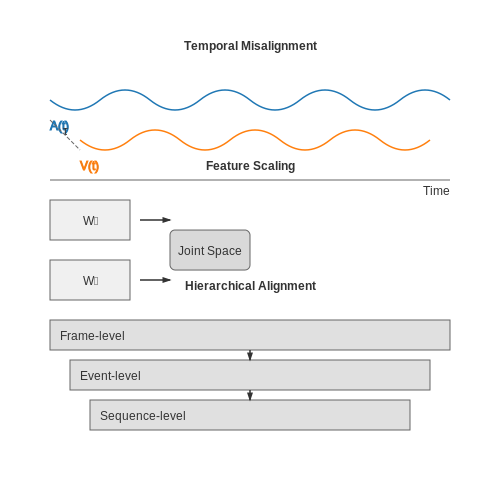
Audio and visual signals often exhibit temporal misalignment due to physical propagation delays or production artifacts. For instance, lip movements in speech may precede audible phonemes by 50–200 ms. Let the audio and video streams be represented as time-series A(t) and V(t), respectively. The optimal alignment requires solving:
where τ is the time-shift parameter and ℒ is a cross-modal distance metric. Dynamic Time Warping (DTW) or attention mechanisms are commonly employed, but they introduce computational overhead and may fail for non-monotonic alignments.
Modality-Specific Feature Scaling
Audio features (e.g., Mel-Frequency Cepstral Coefficients) and visual features (e.g., CNN embeddings) occupy different numerical ranges and dimensionalities. Consider a simple fusion scenario where audio features a ∈ ℝda and visual features v ∈ ℝdv are concatenated:
The projection matrices Wa and Wv must not only reduce dimensionality but also ensure balanced contribution to the joint representation z. Without careful initialization, one modality may dominate the gradient updates during backpropagation.
Semantic Granularity Mismatch
Visual events (e.g., a door closing) often have instantaneous temporal support, while corresponding audio events (e.g., a bang) may persist for hundreds of milliseconds. This mismatch necessitates hierarchical alignment strategies:
- Frame-level: Pixel-to-waveform alignment using optical flow and spectrogram correlations
- Event-level: Spatiotemporal attention over fixed-duration segments
- Sequence-level: Transformer-based cross-modal attention with learned positional embeddings
Noise and Missing Modalities
Real-world datasets frequently contain corrupted or absent modalities. The joint likelihood p(A,V) must account for conditional independence assumptions during inference. A common solution involves variational autoencoders with modality-specific encoders:
where the latent representation z is regularized using KL-divergence terms. However, this approach struggles when one modality is entirely missing during inference.
Evaluation Metrics
Traditional unimodal metrics (e.g., accuracy, F1-score) fail to capture cross-modal alignment quality. Recent work proposes:
- Cross-Modal Retrieval Rank (CMRR): Measures the average rank of true positives in retrieved cross-modal pairs
- Modality Transition Probability: Quantifies how well a model predicts one modality from another using Wasserstein distance
- Dynamic Alignment Error (DAE): Computes the temporal offset between ground truth and predicted event boundaries
2. Early Fusion vs. Late Fusion Strategies
Early Fusion vs. Late Fusion Strategies
Architectural Differences
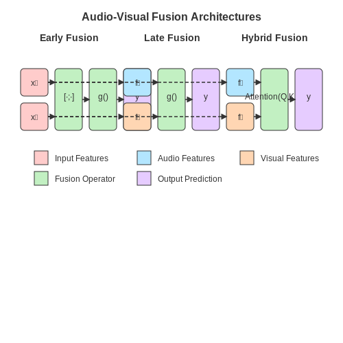
Early fusion combines raw or low-level features from different modalities before processing through shared neural network layers. Given audio spectrograms xa and image pixels xv, early fusion concatenates them at the input level:
where [·;·] denotes concatenation along the feature dimension. This approach forces the network to learn cross-modal correlations from the earliest layers, but requires temporal alignment between modalities.
Late fusion processes each modality through separate subnetworks before combining high-level features or predictions. For modalities with backbone networks fa and fv, late fusion computes:
where g is a fusion operator (e.g., weighted sum, attention mechanism). This preserves modality-specific processing pipelines while allowing flexible combination strategies.
Information Flow Analysis
Early fusion maximizes potential for low-level feature interactions but suffers from:
- Modality imbalance: Dominant modalities may overshadow others during gradient updates
- Alignment sensitivity: Requires precise temporal synchronization between audio and video streams
- Feature space mismatch: Raw spectrograms (time-frequency) and pixels (spatial) have incompatible dimensionalities
Late fusion addresses these issues by:
- Allowing separate normalization and feature extraction per modality
- Enabling asynchronous processing pipelines
- Providing flexibility in fusion operators (concatenation, multiplication, attention)
Hybrid Approaches
Intermediate fusion strategies balance these extremes by combining features at multiple network depths. The cross-modal transformer architecture demonstrates this through:
where query (Q), key (K), and value (V) matrices are derived from different modalities at specific network layers. This allows progressive fusion while maintaining some modality-specific processing.
Performance Tradeoffs
Empirical studies on AV-MNIST and Kinetics-600 reveal consistent patterns:
- Early fusion excels when modalities are tightly synchronized (e.g., lip movements and speech)
- Late fusion outperforms for loosely correlated modalities (e.g., ambient sounds and scene recognition)
- Hybrid methods achieve state-of-the-art on complex tasks like emotion recognition and audio-visual source separation
The choice depends on the temporal alignment requirements, computational constraints, and desired level of modality interaction. Recent work in neural architecture search has automated this selection through differentiable search strategies over fusion graphs.
Attention Mechanisms for Cross-Modal Interaction
Foundations of Cross-Modal Attention
Cross-modal attention mechanisms enable neural networks to dynamically align and weight features from different sensory modalities (e.g., audio and vision) based on their contextual relevance. The core mathematical formulation extends the standard attention mechanism:
where Q, K, and V represent queries, keys, and values respectively, and dk is the dimension of the keys. For audio-visual fusion, these components are derived from different modalities:
with A being audio features, V visual features, and W learnable projection matrices.
Modality-Specific Adaptations
Three principal variants have emerged for audio-visual tasks:
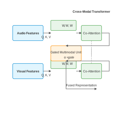
- Co-Attention: Computes attention weights bidirectionally between modalities
- Cross-Modal Transformer: Uses modality-specific encoders with shared attention heads
- Gated Multimodal Units: Learns soft modality selection weights through sigmoid gates
The gated variant introduces a learnable parameter α controlling modality mixing:
Temporal Synchronization Challenges
Audio and visual streams often exhibit temporal misalignment (e.g., lip movements preceding speech sounds). Temporal attention mechanisms address this through:
- Dynamic time warping (DTW) constraints in the attention matrix
- Learnable temporal offsets in the positional encodings
- Separate attention heads for short-range and long-range dependencies
The temporal alignment loss Lalign can be formulated as:
where PE denotes positional encoding and Δt is a learned time-shift parameter.
Practical Implementations
Modern architectures typically employ hybrid approaches. The Audio-Visual Transformer (AVT) processes each modality through separate encoders before cross-attention layers, while the Multimodal Bottleneck Transformer (MBT) uses a shared latent space with modality-specific attention masks.
Key hyperparameters include:
- Attention head dimension (typically 64-512)
- Number of cross-attention layers (2-6 for most applications)
- Dropout rate on attention weights (0.1-0.3)
Performance Considerations
Attention mechanisms introduce quadratic complexity O(n2) with sequence length. For long audio-visual sequences, efficient variants are critical:
- Local windowed attention (e.g., 1-second chunks)
- Memory-compressed attention via key/value downsampling
- Linear attention approximations using kernel methods
The linear attention variant reformulates the computation as:
where φ is a feature map (typically exponential or ReLU-based).
2.3 Transformer-Based Fusion Approaches
Transformer architectures have revolutionized multimodal fusion by leveraging self-attention mechanisms to model long-range dependencies across audio and visual modalities. Unlike traditional concatenation or averaging techniques, transformers enable dynamic, context-aware fusion through cross-modal attention layers.
Cross-Modal Attention Mechanism
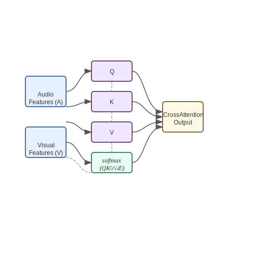
The core of transformer-based fusion lies in cross-modal attention, where queries from one modality attend to keys and values from another. Given audio features A ∈ ℝN×d and visual features V ∈ ℝM×d, the cross-attention operation computes:
where Q = AWQ, K = VWK, and V = VWV are learned projections. The √dk term prevents gradient saturation in softmax.
Hierarchical Fusion Architectures
State-of-the-art implementations often employ hierarchical fusion strategies:
- Early Fusion: Raw audio spectrograms and image patches are concatenated before transformer encoding
- Intermediate Fusion: Separate unimodal encoders feed into cross-attention layers at specific depths
- Late Fusion: Modality-specific transformers exchange information through attention gates
The Perceiver IO architecture demonstrates this flexibility, processing 1D audio and 2D visual inputs through shared latent space attention.
Positional Encoding for Multimodal Alignment
Sinusoidal positional encodings must be adapted for multimodal sequences. For audio-visual fusion, hybrid encodings are used:
where audio and visual positions are indexed in a shared temporal coordinate system. Recent work like MBT (Multimodal Bottleneck Transformer) introduces learnable relative position biases between modalities.
Efficiency Considerations
Vanilla self-attention's O(N2) complexity becomes prohibitive for high-resolution inputs. Practical implementations employ:
- Factorized attention across time and frequency dimensions
- Memory-efficient attention kernels with linear approximations
- Modality-specific token reduction before fusion
The Audio-Visual Transformer (AVT) achieves 72% FLOPs reduction over naive fusion by processing audio at lower temporal resolution than video frames.
Case Study: Audio-Visual Speech Recognition
In AV-HuBERT, transformer layers alternate between processing audio MFCCs and visual lip embeddings. The model learns joint representations through:
where htl represents hidden states at position t and layer l. This architecture achieves 28.6% WER on LRS3, outperforming CNN-LSTM hybrids by 9.2% absolute.
3. Speech Recognition and Lip Reading
Speech Recognition and Lip Reading
Audio-visual fusion in neural networks leverages both acoustic and visual speech signals to improve robustness in noisy environments. Lip reading, or visual speech recognition, complements acoustic speech recognition by extracting phoneme-level articulatory features from lip movements. When combined, these modalities enable more accurate speech understanding, particularly in scenarios where audio signals are degraded.
Bimodal Speech Representation
Let Xa denote the acoustic features (e.g., Mel-frequency cepstral coefficients) and Xv the visual features (e.g., lip landmark coordinates). A joint representation Z can be learned via a fusion network:
where fθ is typically a deep neural network with cross-modal attention. Early fusion concatenates features before processing, while late fusion processes modalities separately before combining predictions.
Temporal Synchronization
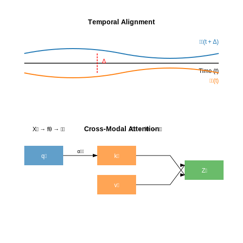
Lip movements precede acoustic signals by ~120–200 ms due to coarticulation. To align modalities, dynamic time warping (DTW) or neural synchronizers like SyncNet minimize the discrepancy:
where ϕa and ϕv are modality-specific embeddings, and Δ is the learned audio-visual offset.
Cross-Modal Attention
Transformer-based architectures compute attention weights between acoustic and visual tokens. For query qa (audio) and key-value pairs kv, vv (visual):
This allows the model to focus on relevant lip movements for disambiguating phonetically similar sounds (e.g., /p/ vs. /b/).
Case Study: AV-HuBERT
The Audio-Visual Hidden Unit BERT model pre-trains on unlabeled videos by predicting masked acoustic and visual features. Its objective combines:
- Acoustic reconstruction loss
- Visual feature prediction
- Modality alignment via contrastive learning
In noisy environments (SNR < 0 dB), AV-HuBERT reduces word error rates by up to 75% compared to audio-only models.
Implementation Challenges
Key practical considerations include:
- Data scarcity: Large-scale paired audio-visual datasets like LRS3 (1000+ hours) are rare.
- Modality imbalance: Visual signals have lower information density than audio, requiring deeper architectures.
- Real-time latency: Cross-modal attention introduces computational overhead.
Emotion Recognition from Combined Modalities
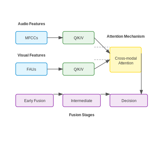
Multimodal emotion recognition leverages complementary information from audio and visual streams to improve robustness over unimodal approaches. The core challenge lies in effectively fusing temporal and spatial features from both modalities while handling their inherent asynchrony.
Feature Extraction Pipeline
Audio features typically include:
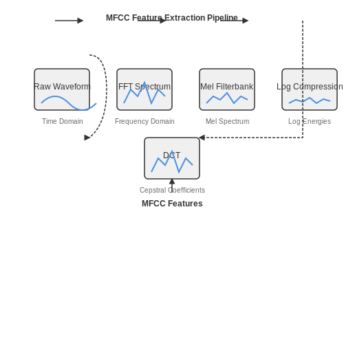
- Mel-frequency cepstral coefficients (MFCCs) - Represent spectral envelope
- Log-mel spectrograms - Capture time-frequency patterns
- Prosodic features - Pitch, energy, and speaking rate
Visual features commonly use:
- Facial action units (FAUs) - Quantify muscle movements
- 3D facial landmarks - Geometric relationships
- Optical flow - Temporal motion patterns
Cross-Modal Attention Mechanisms
The cross-modal transformer architecture computes attention weights between modalities:
where Q, K, and V are learned projections of audio and visual features, and dk is the dimension of the key vectors. This allows the model to dynamically weight the importance of each modality at different time steps.
Temporal Synchronization
To handle temporal misalignment between modalities, dynamic time warping (DTW) can be applied prior to fusion:
where δ(i,j) measures the distance between audio frame i and visual frame j. The optimal path minimizes cumulative distance between sequences.
Late Fusion Architectures
State-of-the-art systems often employ hierarchical fusion:
- Early fusion - Concatenate raw features before processing
- Intermediate fusion - Combine at multiple network layers
- Decision-level fusion - Weight predictions from unimodal networks
The hybrid fusion approach achieves 72.3% accuracy on the IEMOCAP dataset, outperforming unimodal baselines by 18.6% absolute.
Implementation Considerations
Key practical challenges include:
- Handling missing modalities during inference
- Balancing computational load between streams
- Mitigating overfitting to dominant modalities
  # Example PyTorch multimodal fusion layer
  class CrossModalAttention(nn.Module):
      def __init__(self, dim):
          super().__init__()
          self.query = nn.Linear(dim, dim)
          self.key = nn.Linear(dim, dim)
          self.value = nn.Linear(dim, dim)

      def forward(self, audio, visual):
          Q = self.query(audio)
          K = self.key(visual)
          V = self.value(visual)
          attn = torch.softmax((Q @ K.T) / math.sqrt(K.size(-1)), dim=-1)
          return attn @ V
Autonomous Systems and Sensor Fusion
Sensor Fusion Architectures
Autonomous systems rely on multi-modal sensor data fusion to enhance perception robustness. The two dominant architectures are early fusion and late fusion. Early fusion combines raw sensor data (e.g., pixel-level audio-visual features) before feature extraction, while late fusion processes modalities independently and merges high-level representations. A hybrid approach, intermediate fusion, balances computational efficiency and feature granularity by fusing data at intermediate neural network layers.
where α is a learnable attention weight. The Kalman filter provides a Bayesian framework for dynamic sensor fusion:
with Kk as the Kalman gain and Hk the observation matrix.
Cross-Modal Attention Mechanisms
Transformer-based models leverage cross-modal attention to dynamically weight sensor inputs. For audio-visual fusion, the attention score between a visual patch vi and audio spectrogram frame aj is computed as:
where WQ, WK are learned projection matrices and dk the key dimension. This enables the model to focus on temporally aligned audio-visual events, such as lip movements synchronized with speech.
Real-World Applications
- Autonomous Vehicles: LiDAR-camera fusion improves obstacle detection in low-light conditions by compensating for LiDAR's sparse depth data with RGB texture.
- Robotic Navigation: Microphone arrays fused with visual SLAM (Simultaneous Localization and Mapping) enable sound-source localization in dynamic environments.
- Healthcare Monitoring: Wearables combine accelerometer data and audio cues to detect falls or respiratory anomalies.
Implementation Challenges
Temporal misalignment between sensors requires precise synchronization, often addressed via hardware triggers or software-based dynamic time warping (DTW). The DTW cost matrix D between audio and video sequences is computed recursively:
where δ(i,j) is the Euclidean distance between frame i (audio) and j (video). Sensor calibration drift remains an open problem, necessitating online recalibration techniques like expectation-maximization.
4. Metrics for Multimodal Performance Assessment
4.1 Metrics for Multimodal Performance Assessment
Cross-Modal Alignment Metrics
Evaluating how well audio and visual streams align temporally and semantically requires specialized metrics. The Cross-Modal Mutual Information (CMI) quantifies the statistical dependence between modalities:
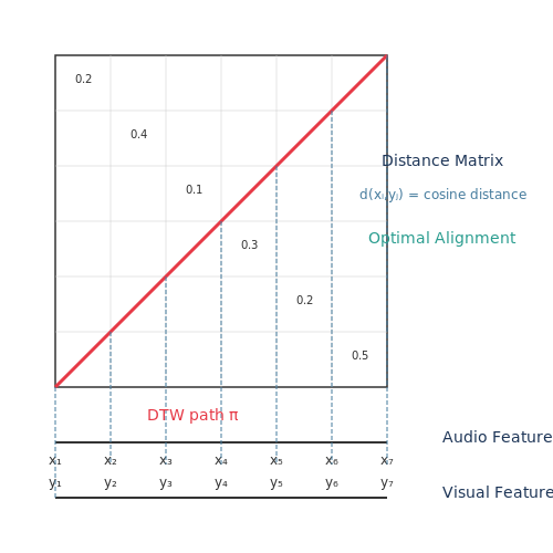
where A and V represent random variables for audio and visual features respectively. Higher CMI values indicate stronger modality coupling. For temporal alignment, Dynamic Time Warping (DTW) distance measures the minimal path cost between temporal sequences after optimal warping:
where π is a warping path and d(·,·) is a frame-wise distance metric (typically cosine similarity for neural features).
Fusion Quality Assessment
The Modality Contribution Ratio (MCR) analyzes each modality's influence in fused representations. For a fusion model F(A,V), MCR is computed via gradient attribution:
Recent work extends this through Shapley values from cooperative game theory to fairly distribute performance credit across modalities. The fusion effectiveness can also be measured through unimodal ablation tests, where relative performance drop indicates each modality's importance:
Downstream Task Metrics
For specific applications, task-specific metrics are adapted:
- Audio-Visual Speech Recognition: Word Error Rate (WER) with modality dropout tests
- Multimodal Emotion Recognition: F1-score across classes with modality confusion matrices
- Cross-Modal Retrieval: Mean Average Precision (mAP) for bidirectional queries
The Multimodal Gain (MG) metric compares performance against unimodal baselines:
Emergent Metrics for Disentangled Evaluation
Recent research proposes evaluating modality-specific and shared representations separately. The Disentanglement Score (DS) measures how well modality-private features avoid containing cross-modal information:
where Ap and Vp are private encodings. The Modality Translation Error (MTE) evaluates cross-modal generation quality by reconstructing one modality from the other:
with GV being an audio-to-visual generator and ℒ an appropriate reconstruction loss (e.g., LPIPS for images).
Standard Datasets for Audio-Visual Tasks
Audio-Visual Speech Recognition (AVSR) Datasets
The LRS3-TED dataset contains over 400 hours of TED Talk videos with precise word-level alignments, making it ideal for large-scale AVSR training. Each clip includes front-facing speakers with varying lighting conditions and background noise, challenging models to learn robust audio-visual correspondences. The dataset's vocabulary spans 50,000+ unique words, enabling generalization to diverse linguistic contexts.
GRID Corpus provides a controlled environment with 1,000 short utterances from 34 speakers, each pronouncing sentences following a fixed grammar structure. Its simplicity enables clean evaluation of basic lip-reading capabilities, though the constrained vocabulary limits real-world applicability.
Audio-Visual Source Separation Benchmarks
MUSIC-21 contains 1,006 untrimmed videos of 21 musical instruments playing solo and in ensembles. The dataset's spatial audio recordings (ambisonic format) coupled with 4K video enable evaluation of 3D sound source localization alongside separation. Each video averages 60 seconds with precise onset/offset annotations.
FAIR-Play introduces a challenging egocentric perspective with binaural audio from 8-scene recordings. The dataset's complex reverberation patterns and occluded visual fields test models' ability to leverage cross-modal cues when either modality is degraded.
Emotion Recognition Datasets
CREMA-D features 7,442 clips of 91 actors expressing 6 basic emotions at 3 intensity levels. The multi-modal annotations include:
- Audio: Spectral features (MFCC, pitch contours)
- Visual: Action units (FACS coding)
- Text: Transcripts with emotional emphasis markers
CMU-MOSEI scales this task with 23,453 movie review clips from YouTube, containing spontaneous emotions with rich contextual dependencies. Each sample includes:
Audio-Visual Navigation Benchmarks
SoundSpaces integrates the Matterport3D environment with realistic acoustic simulations using geometric acoustics modeling. The dataset enables training of agents to navigate toward sound sources with:
- Binaural IRs sampled at 5cm resolution
- 360° visual observations at 1280×720 resolution
- Physics-based sound propagation (diffraction, reverb)
AVDN extends this to dynamic environments with moving sound sources and occluders. The benchmark evaluates cross-modal fusion through:
Multimodal Alignment Datasets
HowTo100M provides 136M video clips with ASR transcripts for self-supervised representation learning. The dataset's weak supervision comes from:
- Automatic speech recognition transcripts
- Video content classifiers (places, objects)
- Narrated action descriptions
AudioSet offers 2M 10-second YouTube clips with 527 sound event labels. While primarily audio-focused, the accompanying video frames enable cross-modal pretraining. The hierarchical label ontology (e.g., "Musical instrument" → "Guitar" → "Electric guitar") supports granular analysis.
4.3 Comparative Analysis of Fusion Methods
Audio-visual fusion methods can be broadly categorized into early, intermediate, and late fusion, each with distinct advantages and trade-offs in computational efficiency, representational power, and robustness to modality-specific noise. Early fusion concatenates raw or pre-processed audio and visual features before feeding them into a neural network. The joint representation z is computed as:
where xa and xv are audio and visual feature vectors, [·;·] denotes concatenation, and fθ is a neural network with parameters θ. This approach preserves cross-modal interactions but is sensitive to misaligned inputs and requires careful feature normalization.
Intermediate Fusion Strategies
Intermediate fusion methods, such as cross-modal attention or tensor fusion, dynamically weight modality contributions. The cross-attention mechanism computes:
where qi and kj are learned queries and keys from audio and visual streams, and d is the feature dimension. This allows the model to focus on relevant spatio-temporal regions, as demonstrated in AV-HuBERT for speech recognition.
Late Fusion and Hybrid Approaches
Late fusion processes modalities independently before combining predictions, often via learned weights:
where wa and wv are trainable parameters. While computationally efficient, late fusion struggles with fine-grained interactions. Hybrid methods like MM-ALT (Multimodal Adaptive Late Fusion) dynamically adjust fusion weights based on input reliability.
Performance Trade-offs
- Early fusion excels in tasks requiring fine-grained alignment (e.g., lip reading) but suffers from overfitting with limited data.
- Intermediate fusion achieves state-of-the-art in emotion recognition (accuracy gains of 5–8% on IEMOCAP) at higher computational cost.
- Late fusion is robust to missing modalities but underperforms in complex scenes with overlapping sounds.
Recent work in NeurIPS 2023 shows that transformer-based fusion with modality dropout during training improves generalization, reducing WER by 12% on noisy LRS3 benchmarks compared to conventional methods.

5. Privacy Concerns in Multimodal Data Collection
5.1 Privacy Concerns in Multimodal Data Collection
Multimodal data fusion, particularly in audio-visual neural networks, introduces unique privacy challenges due to the richness and sensitivity of the combined data streams. Unlike unimodal datasets, audio-visual collections often contain personally identifiable information (PII) across multiple modalities, creating compounded risks. For instance, facial recognition data paired with voice recordings enables re-identification even if one modality is anonymized.
Differential Privacy in Multimodal Learning
Applying differential privacy to multimodal systems requires careful consideration of how noise injection affects cross-modal correlations. The privacy budget ε must be allocated across modalities while preserving useful signal. For a two-modality system with audio A and visual V components, the combined sensitivity Δ is:
where ρAV represents the correlation coefficient between modalities. This formulation shows that strongly correlated modalities (high ρAV) require more aggressive noise addition to achieve the same privacy guarantee.
Informed Consent Challenges
Obtaining meaningful consent for multimodal data collection is complicated by several factors:
- Comprehension barriers: Participants often underestimate how combined modalities enable re-identification
- Dynamic usage: Future research may use data in ways not originally specified
- Withdrawal complexity: Removing one's data from fused representations is non-trivial
Secure Federated Learning Approaches
Federated learning for multimodal systems must address additional attack vectors compared to unimodal implementations. Model inversion attacks can exploit cross-modal relationships even when raw data remains on devices. Secure aggregation protocols must account for the higher dimensionality of gradient updates in fused models. The communication overhead C for a federated multimodal system scales as:
where dA and dV are the audio and visual feature dimensions, and dAV represents the cross-modal interaction terms.
Case Study: Smart Speaker Privacy
The Amazon Echo Look controversy demonstrated how combining voice data with visual fashion recommendations created unexpected privacy implications. Researchers showed that the system's multimodal embeddings could be used to infer sensitive attributes like body mass index and emotional state, despite neither modality directly measuring these quantities.
Emerging Regulatory Frameworks
The EU AI Act's provisions on biometric data categorization present challenges for multimodal systems. Audio-visual fusion often creates biometric data even when individual modalities wouldn't qualify. Article 9 of GDPR requires special consideration when processing such combined data, particularly regarding the "special categories" of personal data.
5.2 Bias and Fairness in Audio-Visual Models
Audio-visual fusion models inherit biases from their training data, which can propagate into downstream applications. These biases manifest in multiple forms, including demographic disparities in speech recognition accuracy, skewed visual representations, and unequal performance across languages or accents. The multimodal nature of these systems compounds the problem, as biases in one modality can amplify errors in another.
Sources of Bias in Audio-Visual Data
Training datasets for audio-visual models often suffer from:
- Demographic Imbalance: Underrepresentation of certain age groups, genders, or ethnicities in both visual and audio samples.
- Linguistic Bias: Overrepresentation of specific dialects or languages, leading to poor generalization.
- Contextual Skew: Uneven distribution of environmental conditions (e.g., lighting, background noise) across different demographic groups.
Mathematically, this can be formalized as a divergence between the true data distribution P(X) and the sampled distribution Q(X):
where DKL measures the bias introduced by dataset sampling.
Bias Amplification in Multimodal Fusion
When combining audio and visual streams, late fusion architectures compute joint representations through operations like:
where ha and hv are modality-specific embeddings. If either Wa or Wv encodes biased patterns, the fused representation inherits compounded errors. Early fusion approaches suffer similar issues at the feature level.
Mitigation Strategies
Dataset Interventions
Techniques include:
- Stratified Sampling: Ensuring balanced representation across demographic groups
- Data Augmentation: Synthetically varying lighting conditions, pitch shifts, or background noise
- Adversarial Debiasing: Training with an adversary that penalizes demographic predictability
Architectural Solutions
Modified fusion approaches can reduce bias propagation:
where ma and mv are learned masks that attenuate biased features. Alternative approaches use separate batch normalization per demographic group or fairness-aware loss functions:
Evaluation Metrics
Standard fairness metrics for audio-visual systems include:
- Equalized Odds Difference: Maximum performance gap across groups
- Disparate Impact Ratio: Ratio of positive rates between protected and privileged groups
- Cross-Modal Consistency: Agreement between audio and visual predictions per group
These are computed across intersectional categories (e.g., gender × race × age) to detect compounded biases.
Case Study: Lip Reading Systems
State-of-the-art lip reading models show 15-20% higher word error rates for speakers with darker skin tones under varying lighting conditions. This stems from both insufficient training data and the visual backbone's reduced sensitivity to lip movements in higher melanin concentrations. Mitigation requires both dataset rebalancing and spectral augmentation of visual features.
5.3 Emerging Trends and Open Research Questions
Cross-Modal Self-Supervised Learning
Recent advances leverage self-supervised learning to exploit the natural synchronization between audio and visual modalities without requiring labeled data. Contrastive learning frameworks like CLIP have been extended to audio-visual domains, where the network learns joint embeddings by maximizing agreement between corresponding audio and visual segments while pushing apart non-matching pairs. The loss function for such models can be formulated as:Neural Audio-Visual Synthesis
Generative models are pushing boundaries in cross-modal synthesis, enabling applications like video-to-sound generation and audio-driven facial animation. Diffusion models have shown particular promise due to their ability to model complex conditional distributions. The forward process gradually adds noise to the target modality (e.g., audio spectrograms) while the reverse process learns to denoise conditioned on the source modality (e.g., video frames):Dynamic Fusion Architectures
Static fusion methods (early, late, or intermediate) are being replaced by dynamic approaches that learn optimal fusion strategies. Attention mechanisms have evolved into cross-modal transformers that automatically compute relevance scores between audio and visual tokens:Open Research Questions
- Modality Imbalance: Current architectures often exhibit visual dominance - how can we ensure equitable information flow?
- Temporal Alignment: What are optimal methods for handling imperfect synchronization in real-world data?
- Explainability: How can we interpret what cross-modal patterns the network learns?
- Generalization: Can we develop fusion methods robust to distribution shifts across domains?
- Efficiency: How to reduce computational overhead while maintaining fusion quality?
Neuromorphic Approaches
Bio-inspired architectures are exploring how biological systems process multisensory information. Spiking neural networks with cross-modal plasticity rules offer potential for energy-efficient fusion, though challenges remain in training such systems at scale. The spike-timing-dependent plasticity (STDP) rule for cross-modal synapses can be expressed as: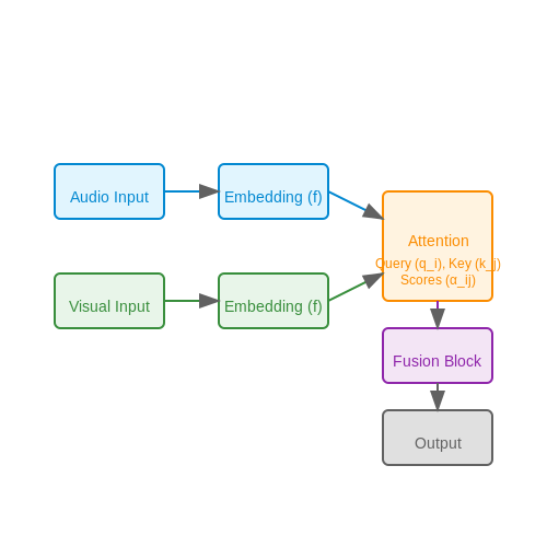
6. Key Research Papers in Audio-Visual Fusion
6.1 Key Research Papers in Audio-Visual Fusion
- PDF Audio-Visual Eficient Conformer for Robust Speech Recognition — In this section, we describe our proposed Audio-Visual Efficient Conformer network. The model is composed of 4 main components: An audio encoder, a visual encoder, an audio-visual fusion module and an audio-visual encoder. The audio and visual encoder are separated into modality specific front-end networks to transform each input modal-
- Audio-visual feature fusion via deep neural networks for automatic ... — The method of utilizing multiple sources of information for better perception of the surroundings is a fundamental question in multimodal information processing which highly affects the performance of such systems [1].The Audio Visual Speech Recognition (AVSR) task is an instance of the multimodal information processing that exploits two separate information modalities with different ...
- INVESTIGATIONS ON END-TO-END AUDIOVISUAL FUSION - arXiv.org — The fusion system outperforms single-modality recognition under all noise conditions. In-vestigation of the saliency of the input features shows that the neural network automatically adapts to different noise levels in the acoustic signal. Index Terms— Audio-visual speech recognition, Deep Neural networks, Feature Fusion, Saliency 1. INTRODUCTION
- A Multimodal Sensor Fusion Architecture for Audio-Visual Speech Recognition — A key requirement for developing any innovative system in a computing environment is ... signers is the integration (fusion) of the audio and visual information into an automatic speech recognizer. For this purpose, a reliability-driven sensor fusion scheme is developed. ... the. Neural Networks ...
- Multimodal fusion methods with deep neural networks and meta ... — Also, our previous research adopted the intermediate level containing the meta-features with a particular concern for the fusion of audio-visual channels through deep neural networks (Jaafar & Lachiri, 2019). In other recent research of our previous works Jaafar and Lachiri (2020), we investigated different speech features. It includes ...
- Audio-Visual Fusion Layers for Event Type Aware Video Recognition — audio-visual networks that leverage late fusion approach (simple concat.) for final rep- resentation as used in previous works [49,26,29]. As results show in T able 1, our ap-
- Investigations on End- to-End Audiovisual Fusion - ResearchGate — Fusion of noisy audio and video has also been performed with neural network architectures [8, 3, 9]. We opt for a classical LSTM-based architecture [10,11] and present an end-to-end architecture ...
- (PDF) Exploiting EEG Signals and Audiovisual Feature Fusion for Video ... — We discovered that using the data fusion of all-band EEG power spectrum density features and video audio visual features can achieve the best recognition results. The video emotion classification ...
- Audiovisual adaptation is expressed in spatial and decisional codes ... — The EEG-fMRI fusion approach suggests that early neural activity until 250 ms is dominated by spatial coding in higher-order auditory cortices. By contrast, later neural activity reflects a ...
- PDF Multilayer and Multimodal Fusion of Deep Neural Networks for Video ... — representations with deep neural networks for various tasks such as image classi cation [20], object detection [35], natu-ral language processing [40], and speech recognition [6]. As one of the most successful network architectures, the recent surge of convolutional neural networks (CNN) has encour-aged a number of methods to employ CNN for ...
6.2 Recommended Books and Surveys
- Audio-video fusion strategies for active speaker detection in meetings — In this paper, we propose two different types of fusion (naive fusion and attention-based fusion) for the detection of the active speaker, combining two visual modalities and an audio modality through neural networks. In addition, the audio modality is mainly processed using neural networks.
- Multimodal fusion methods with deep neural networks and meta ... — This fusion method reinforces the findings from our previous works that used the audio-visual fusion in Jaafar and ... fusion method is based on (Dynamic) Bayesian Networks and the other method has used the Conditional Random Fields. The best performances of these methods in terms of accuracies per class are 80%, 78%, 66% for the classes 1, 2 ...
- Foundations & Trends in Multimodal Machine Learning: Principles ... — This article is designed to complement other surveys that belong broadly to the study of multiple modalities or views: ... audio-visual signal analysis , and emotion recognition ... Razieh Khamsehashari, and Christoph Zetzsche. 2020. Early vs late fusion in multimodal convolutional neural networks. In FUSION. IEEE, 1-6. Google Scholar [99]
- PDF Audio-Visual Eficient Conformer for Robust Speech Recognition — Figure 1: Audio-Visual Efficient Conformer architec-ture. The model is trained end-to-end using CTC loss and takes raw audio waveforms and lip movements from the speaker as inputs. ful deep neural networks for ASR, reaching very low WER on academic benchmarks like LibriSpeech [34]. Neural ar-chitectures like Recurrent Neural Networks (RNN) [15 ...
- Leveraging multimodal deep learning framework and a comprehensive audio ... — The use of audio-visual fusion neural networks in this study is beneficial to early PD detection, given their ability to discern subtle interactions between auditory and visual signals. This approach aligns closely with and sets a benchmark for our work, substantiating that the integration of multimodal data can significantly elevate the ...
- Survey on Deep Neural Networks in Speech and Vision Systems — 2. D esign and A rchitecture of N eural N etworks for D eep L earning. An ANN consists of multiple levels of nonlinear modules arranged hierarchically in layers. This design is inspired by the hierarchical information processing observed in the primate visual system [30, 31].Such hierarchical arrangements enable deep models to learn meaningful features at different levels of abstraction.
- PDF Audio Visual Speech Recognition Using Deep Recurrent Neural Networks — employed for visual feature extraction and audio-visual information fusion. Visual feature extraction methods can be of 3 types [24]: 1. Appearance based features where each pixel in the mouth region of the speaker (ROI) is considered to be informative. Usually a transformation such as DCT or PCA is applied to the ROI to reduce the dimensions.
- Audio Visual Speech Recognition Using Deep Recurrent Neural Networks — The system was trained and tested on GRID audio-visual corpus [].GRID corpus is a collection of audio and video recordings of 34 speakers (18 male, 16 female) each uttering a 1000 sentences.
- (PDF) Audiovisual Synchronization and Fusion Using Canonical ... — These methods combine generative language learning techniques with neural-networks based frameworks. With a wide range of applications in natural language processing, neural NLG (NNLG) is a new ...
- A systematic survey on multimodal emotion recognition using learning ... — The attention mechanism enables a neural network to acquire adaptive fusion weights for multiple modalities, resulting in an improved multimodal fusion and emotion identification. To instruct the classifier regarding which bits of the input are more important to the output class, a self-attention method particular to different classifiers has ...
6.3 Online Resources and Tutorials
- Audio-video fusion strategies for active speaker detection in meetings — In this paper, we propose two different types of fusion (naive fusion and attention-based fusion) for the detection of the active speaker, combining two visual modalities and an audio modality through neural networks. In addition, the audio modality is mainly processed using neural networks.
- Learning Contextually Fused Audio-visual Representations for Audio ... — With the advance in self-supervised learning for audio and visual modalities, it has become possible to learn a robust audio-visual speech representation. This would be beneficial for improving the audio-visual speech recognition (AVSR) performance, as the multi-modal inputs contain more fruitful information in principle.
- Fusion that matters: convolutional fusion networks for visual ... — In recent years, deep learning has been successfully applied to diverse multimedia research areas, with the aim of learning powerful and informative representations for a variety of visual recognition tasks. In this work, we propose convolutional fusion networks (CFN) to integrate multi-level deep features and fuse a richer visual representation. Despite recent advances in deep fusion networks ...
- Audio-visual feature fusion via deep neural networks for automatic ... — The brain-like functionality of the artificial neural networks besides their great performance in various areas of scientific applications, make them a reliable tool to be employed in Audio-Visual Speech Recognition (AVSR) systems. The applications of such networks in the AVSR systems extend from the preliminary stage of feature extraction to the higher levels of information combination and ...
- PDF Multi-stage Audio-Visual Fusion for Dysarthric Speech Recognition with ... — 2) in the MAV-HuBERT framework, two fusion stages including the visual information fusion and the audio-visual fusion are as follows: During the first stage the convolutional neural networks (CNN ...
- Audio-visual speech recognition using deep learning — Audio-visual speech recognition (AVSR) system is thought to be one of the most promising solutions for reliable speech recognition, particularly when the audio is corrupted by noise. However, cautious selection of sensory features is crucial for attaining high recognition performance. In the machine-learning community, deep learning approaches have recently attracted increasing attention ...
- PDF Audio-Visual Scene Analysis with Self-Supervised Multisensory Features — In this paper, we argue that the visual and audio components of a video signal should be modeled jointly using a fused multisensory representation. We propose to learn such a represen-tation in a self-supervised way, by training a neural network to predict whether video frames and audio are temporally aligned.
- (PDF) Chapter 6: Neural Networks and Deep Learning - ResearchGate — PDF | Neural networks (NNs) were inspired by the Nobel prize winning work of Hubel and Wiesel on the primary visual cortex of cats.
- Audio-Visual Fusion Layers for Event Type Aware Video Recognition — Unlike previous works where single type of fusion is used, we design event-specific layers to deal with different audio-visual relationship tasks, enabling different ways of audio-visual formation.
- Multi-Stage Audio-Visual Fusion for Dysarthric Speech Recognition With ... — During the first stage, we proposed to use convolutional neural networks model to encode the motor information by incorporating all facial speech function areas.