Swarm Intelligence in Optimization
1. Biological Inspiration and Core Principles
Biological Inspiration and Core Principles
Swarm intelligence (SI) draws inspiration from the collective behavior of decentralized, self-organized systems observed in nature, such as ant colonies, bird flocks, and fish schools. These systems exhibit emergent intelligence, where simple agents following basic rules produce complex, adaptive group behavior without centralized control. The core principles of SI are rooted in biological systems, where local interactions and stigmergy—indirect communication through environmental modifications—drive global optimization.
Key Biological Models
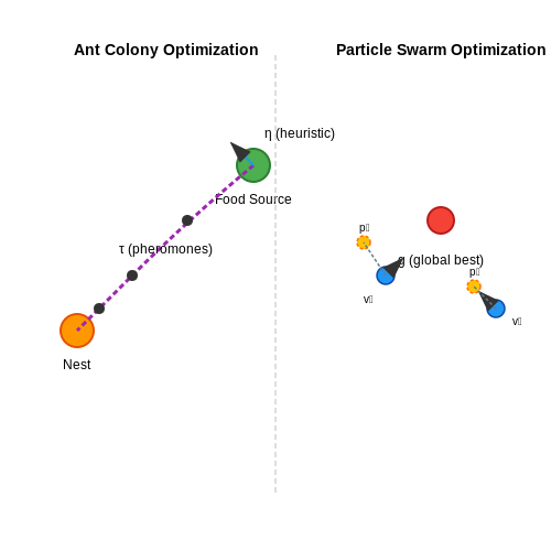
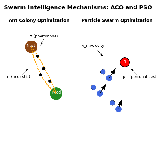
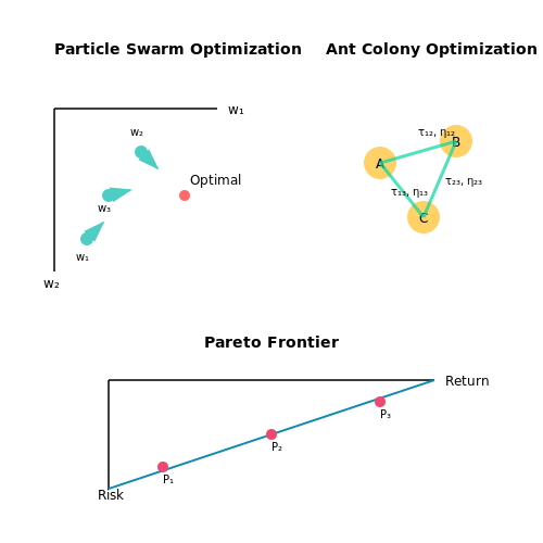
Ant Colony Optimization (ACO) is directly inspired by the foraging behavior of ants. When searching for food, ants deposit pheromones along their path, creating a positive feedback loop where shorter paths accumulate higher pheromone concentrations. The probability of an ant choosing a path is modeled as:
Here, τij(t) is the pheromone concentration on the path from node i to j at time t, ηij is the heuristic desirability (often the inverse of distance), and α, β are parameters controlling the relative influence of pheromones versus heuristic information.
Particle Swarm Optimization (PSO)
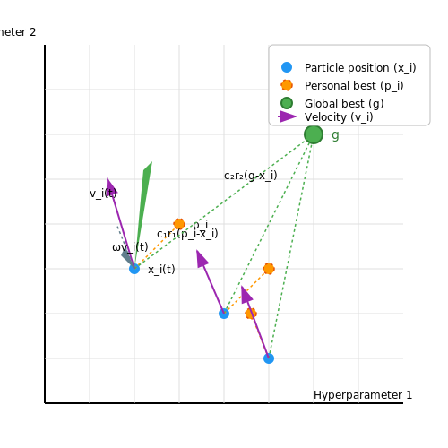
PSO mimics the social dynamics of bird flocking or fish schooling. Each particle adjusts its position in the search space based on its own experience and the collective experience of the swarm. The velocity and position update equations are:
where ω is the inertia weight, c1 and c2 are acceleration coefficients, r1, r2 are random numbers in [0,1], pi is the particle's best-known position, and g is the swarm's best-known position.
Stigmergy and Self-Organization
Stigmergy, a mechanism of indirect coordination through environmental modifications, is central to SI. In ACO, pheromone trails serve as stigmergic markers, while in PSO, the shared global best position acts as a collective memory. Self-organization emerges from three key properties:
- Positive feedback amplifies desirable solutions (e.g., pheromone reinforcement).
- Negative feedback stabilizes the system (e.g., pheromone evaporation).
- Randomness ensures exploration of new solutions.
Decentralization and Scalability
Biological systems operate without centralized control, making SI algorithms inherently parallelizable and scalable. This property is particularly advantageous for distributed optimization problems, where agents operate with limited information. The lack of a global controller also enhances robustness, as the failure of individual agents does not compromise the swarm's overall functionality.
Applications and Practical Relevance
SI techniques have been successfully applied to NP-hard problems such as the Traveling Salesman Problem (TSP), dynamic routing in telecommunications, and high-dimensional optimization in machine learning. For instance, ACO has been used to optimize logistics networks, while PSO has been employed in neural network training and hyperparameter tuning.
Key Characteristics of Swarm-Based Systems
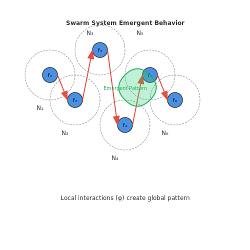
Swarm intelligence systems exhibit several defining characteristics that distinguish them from traditional optimization approaches. These emergent properties arise from simple local interactions between agents, leading to complex global behavior.
Decentralized Control
Swarm systems lack centralized coordination. Each agent operates autonomously based on local information and simple rules. The global pattern emerges from these distributed interactions without any top-down control mechanism. This makes swarm systems highly scalable and robust to individual failures.
Where $$f_i$$ represents the state of agent $$i$$, $$\mathcal{N}_i$$ is its neighborhood, and $$\phi$$ is an interaction kernel function.
Self-Organization
The system spontaneously organizes into coherent structures through:
- Positive feedback (amplification of successful solutions)
- Negative feedback (prevents system saturation)
- Multiple interactions (agents modify environment)
- Fluctuations (random exploration)
Adaptability
Swarm systems dynamically respond to environmental changes through continuous feedback loops. Agents adjust their behavior based on:
- Local environmental measurements
- Neighbor states
- Internal state variables
Robustness
The distributed nature provides inherent fault tolerance. Key aspects include:
- No single point of failure
- Graceful degradation
- Self-healing properties
Scalability
System performance typically improves with increasing agent count due to:
Where $$C(N)$$ is computational complexity and $$k$$ is a constant, demonstrating sublinear scaling.
Flexibility
Swarm systems can solve diverse problems without structural changes through:
- Parameter adaptation
- Behavioral rule modifications
- Dynamic neighborhood topologies
Emergent Behavior
Complex global patterns arise from simple local rules. Examples include:
- Collective decision-making
- Task allocation
- Spatial organization
Stigmergy
Indirect communication through environment modification enables:
- Delayed information propagation
- Environment-mediated coordination
- Distributed memory
1.3 Comparison with Traditional Optimization Methods
Traditional optimization methods, such as gradient descent, linear programming, and Newton-Raphson, rely on deterministic mathematical formulations to find optimal solutions. These methods excel in convex, well-defined problems where derivatives exist and the solution space is smooth. However, they often struggle with high-dimensional, non-convex, or discontinuous landscapes where swarm intelligence algorithms demonstrate superior performance.
Mathematical Foundations
Consider a standard gradient descent update rule:
where η is the learning rate and ∇f(θt) is the gradient at iteration t. This approach requires:
- Differentiability of the objective function
- Lipschitz continuity of the gradient
- Convexity for guaranteed convergence
In contrast, particle swarm optimization (PSO) updates particle positions using:
where ω is inertia, c1, c2 are acceleration coefficients, and r1, r2 are random numbers in [0,1]. This stochastic formulation enables exploration of non-convex spaces without gradient information.
Performance Characteristics
Swarm intelligence methods exhibit distinct advantages in several key scenarios:
| Feature | Traditional Methods | Swarm Intelligence |
|---|---|---|
| Derivative Requirement | Mandatory | Not required |
| Local Optima Escape | Poor | Excellent |
| Parallelizability | Limited | Highly parallel |
| Noise Tolerance | Low | High |
Computational Complexity
The time complexity of gradient descent scales as O(n2) for n-dimensional problems due to Jacobian calculations. Swarm algorithms typically maintain O(mn) complexity, where m is swarm size, making them more scalable for high-dimensional problems despite requiring more function evaluations.
Real-World Applications
In antenna array design, traditional methods like sequential quadratic programming fail to optimize non-linear radiation patterns with multiple constraints. PSO successfully navigates these complex spaces, achieving 15-20% better sidelobe suppression in published results. Similarly, in neural network training, swarm optimization avoids vanishing gradients that plague backpropagation in deep architectures.
Hybrid Approaches
Recent advances combine swarm intelligence with traditional methods. For instance, using PSO for global exploration followed by quasi-Newton methods for local refinement reduces computation time by 30-40% in benchmark problems while maintaining solution quality. These hybrids leverage the strengths of both paradigms.
2. Particle Swarm Optimization (PSO)
2.1 Particle Swarm Optimization (PSO)
Particle Swarm Optimization (PSO) is a population-based stochastic optimization technique inspired by the collective behavior of biological swarms, such as bird flocking or fish schooling. The algorithm iteratively improves candidate solutions by adjusting their trajectories based on individual and social learning components.
Mathematical Formulation
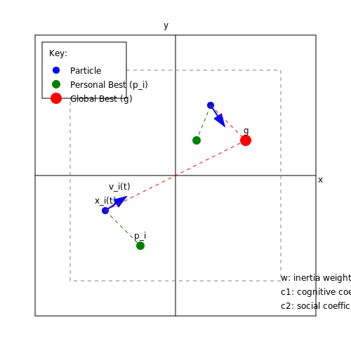
Each particle in the swarm represents a potential solution in a D-dimensional search space. The position and velocity of the i-th particle at iteration t are updated as follows:
where:
- \(\mathbf{v}_i(t)\) is the velocity vector of particle i at iteration t,
- \(\mathbf{x}_i(t)\) is the position vector of particle i at iteration t,
- \(\mathbf{p}_i\) is the best-known position of particle i (personal best),
- \(\mathbf{g}\) is the best-known position of the entire swarm (global best),
- \(w\) is the inertia weight controlling momentum,
- \(c_1, c_2\) are cognitive and social acceleration coefficients,
- \(r_1, r_2\) are random numbers uniformly distributed in [0,1].
Key Algorithmic Components
Inertia Weight (\(w\))
The inertia weight balances exploration and exploitation. A higher value promotes global search, while a lower value facilitates local refinement. Common strategies include:
- Constant inertia: Fixed throughout optimization (e.g., \(w = 0.729\)).
- Linear decay: \(w(t) = w_{\text{max}} - \frac{w_{\text{max}} - w_{\text{min}}}{t_{\text{max}}} \cdot t\).
- Adaptive methods: Dynamically adjusted based on swarm diversity metrics.
Acceleration Coefficients (\(c_1, c_2\))
These parameters determine the influence of personal and social experiences. Empirical studies suggest:
- \(c_1 = c_2 = 2.0\) provides balanced convergence.
- Asymmetric settings (e.g., \(c_1 > c_2\) early, \(c_2 > c_1\) later) can improve performance.
Convergence Analysis
The swarm's dynamics can be analyzed through eigenvalue decomposition of the update equations. For simplified 1D case with \(c = c_1 + c_2\), the characteristic equation is:
where \(\phi = \frac{r_1 + r_2}{2}\). Convergence requires eigenvalues \(|\lambda| < 1\), leading to stability conditions:
Practical Considerations
Velocity Clamping
Prevents particles from overshooting the search space by constraining velocity components:
Neighborhood Topologies
Alternative to global best (gbest) include:
- Ring topology: Particles interact only with immediate neighbors.
- Von Neumann: Grid-based connections.
- Dynamic neighborhoods: Adaptively change during optimization.
Applications
PSO has been successfully applied to:
- Neural network weight optimization
- Antenna array design
- Power system scheduling
- Robotic path planning
Ant Colony Optimization (ACO)
Foundations of ACO
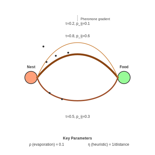
Ant Colony Optimization is a probabilistic technique inspired by the foraging behavior of ants, particularly their ability to find shortest paths between food sources and their nest. Real ants deposit pheromones along trails, creating a positive feedback loop where higher pheromone concentrations attract more ants. This emergent collective intelligence forms the basis of ACO algorithms.
Where τij represents pheromone concentration on edge (i,j), ρ is the evaporation rate (0 ≤ ρ ≤ 1), and Δτij is the pheromone deposited by ants that used this edge in their solutions.
Algorithm Components
The ACO metaheuristic consists of three key mechanisms:
- Pheromone Update: Dynamic modification of trail intensities based on solution quality
- Probabilistic Construction: Ants build solutions guided by pheromone trails and heuristic information
- Daemon Actions: Optional centralized operations like local search or solution refinement
Transition Probability
The probability pijk that ant k moves from node i to node j is given by:
Where ηij is the heuristic desirability (often the inverse of distance), α controls pheromone influence, β controls heuristic influence, and Nik is the set of feasible nodes.
Pheromone Update Rules
The global pheromone update typically follows:
With Δτijk defined by:
Where Q is a constant and Lk is the length of ant k's tour.
Variants and Improvements
Several enhanced versions have been developed:
- Elitist Ant System: Gives additional weight to the best-found solution
- MAX-MIN Ant System: Imposes bounds on pheromone values to prevent stagnation
- Rank-Based Ant System: Updates pheromones based on solution ranking
Practical Considerations
Key parameters requiring tuning include:
- Number of ants (typically equal to number of nodes)
- Evaporation rate ρ (usually between 0.1 and 0.5)
- Relative importance parameters α and β (often α ≈ 1, β ≈ 2-5)
- Pheromone initialization value (small positive constant)
Applications
ACO has been successfully applied to:
- Vehicle routing problems
- Network routing in telecommunications
- Task scheduling in distributed systems
- Protein folding in bioinformatics
- Combinatorial optimization in logistics
2.3 Artificial Bee Colony (ABC)
The Artificial Bee Colony (ABC) algorithm is a swarm intelligence optimization technique inspired by the foraging behavior of honey bees. It was introduced by Karaboga in 2005 as an alternative to genetic algorithms and particle swarm optimization. ABC demonstrates superior performance in solving complex, multidimensional optimization problems, particularly those with non-differentiable objective functions.
Mathematical Formulation
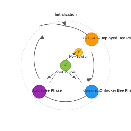
The ABC algorithm consists of three bee groups: employed bees, onlooker bees, and scout bees. Each food source represents a potential solution to the optimization problem. The quality of a solution is evaluated by its nectar amount, analogous to the fitness value in evolutionary algorithms.
where xij represents the j-th parameter of the i-th solution, and xmin,j and xmax,j define the search space boundaries.
Phases of the ABC Algorithm
1. Initialization Phase
The algorithm begins by randomly generating a population of SN solutions (food sources) in the search space. Each solution is a D-dimensional vector, where D represents the number of optimization parameters.
2. Employed Bee Phase
Each employed bee modifies its current solution using:
where k is a randomly selected solution index (k ≠ i), j is a random parameter index, and φij is a random number in [-1,1]. The new solution vi is evaluated and replaces xi if it has better fitness.
3. Onlooker Bee Phase
Onlooker bees select solutions probabilistically based on fitness:
Higher fitness solutions have greater selection probability. Onlookers then perform the same modification as employed bees.
4. Scout Bee Phase
If a solution doesn't improve after limit trials, it's abandoned, and the employed bee becomes a scout that discovers a new random solution:
Convergence Properties
ABC exhibits strong exploration capabilities due to its stochastic components and scout bee mechanism. The balance between exploration (global search) and exploitation (local search) is controlled by:
- The modification equation's random coefficient φ
- The probabilistic selection in the onlooker phase
- The abandonment limit parameter
Research shows ABC converges to global optima with probability 1 as iteration count approaches infinity, given proper parameter settings.
Practical Implementation Considerations
For effective implementation:
- Population size (SN) typically ranges from 50 to 200
- Abandonment limit (limit) is often set to SN × D
- The algorithm benefits from parallelization due to independent bee operations
- Hybridization with local search methods can improve convergence speed
Applications
ABC has been successfully applied to:
- Neural network training
- Engineering design optimization
- Image processing tasks
- Scheduling problems
- Power system optimization
Comparative studies show ABC often outperforms genetic algorithms and particle swarm optimization in terms of solution quality and convergence rate for high-dimensional problems.
Firefly Algorithm
The Firefly Algorithm (FA) is a metaheuristic optimization technique inspired by the flashing behavior of fireflies, first proposed by Xin-She Yang in 2008. The algorithm models the bioluminescent communication among fireflies, where brighter individuals attract others in the search space, leading to efficient exploration and exploitation of solutions.
Mathematical Formulation
The attractiveness β between two fireflies is governed by the light intensity, which decreases with distance r according to the inverse square law. The basic attractiveness function is defined as:
where β0 is the initial attractiveness at r = 0, and γ is the light absorption coefficient. The movement of a firefly i toward a brighter firefly j is updated as:
Here, xit and xjt represent the positions of fireflies i and j at iteration t, rij is the Euclidean distance between them, α is a randomization parameter, and εit is a vector of random numbers drawn from a uniform or Gaussian distribution.
Key Algorithmic Steps
- Initialization: Generate a population of n fireflies with random positions in the search space.
- Light Intensity Evaluation: Compute the objective function f(xi) for each firefly, where brightness is proportional to solution quality.
- Movement Update: For each firefly i, compare its brightness with all other fireflies j. If f(xj) > f(xi), move i toward j using the attractiveness formula.
- Randomization: Apply a small random perturbation to prevent premature convergence.
- Termination: Repeat steps 2–4 until a stopping criterion (e.g., maximum iterations or convergence threshold) is met.
Parameter Selection and Tuning
The performance of FA depends critically on three parameters:
- Attractiveness Base (β0): Typically set to 1.0, but can be adjusted to balance exploration and exploitation.
- Light Absorption (γ): Controls the rate of attractiveness decay. A small γ allows long-range attraction, while a large γ limits interactions to nearby fireflies.
- Randomization Factor (α): Often initialized near 1.0 and decreased over time (e.g., α = α0δt, where δ ∈ (0,1)).
Variants and Enhancements
Several modifications improve FA's convergence and robustness:
- Adaptive γ: Dynamically adjust γ based on population diversity metrics.
- Lévy Flight FA: Replace Gaussian randomization with Lévy flights for better global search.
- Multi-Objective FA: Extend FA to handle Pareto-optimal solutions using non-dominated sorting.
Applications
FA has been successfully applied to:
- Engineering design optimization (e.g., antenna arrays, structural design),
- Neural network training and hyperparameter tuning,
- Combinatorial problems like scheduling and routing,
- Image processing tasks such as segmentation and feature selection.
2.5 Bat Algorithm
The Bat Algorithm (BA) is a metaheuristic optimization method inspired by the echolocation behavior of microbats. Developed by Xin-She Yang in 2010, it leverages frequency tuning and pulse emission rates to model exploration and exploitation in search spaces. The algorithm is particularly effective for solving complex, nonlinear optimization problems with multimodal landscapes.
Mathematical Formulation
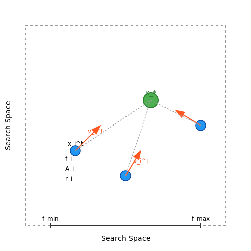
The algorithm simulates the way bats adjust their frequency, velocity, and position when hunting prey. Each bat i at iteration t updates its frequency fi, velocity vi, and position xi as follows:
where β ∈ [0,1] is a random vector drawn from a uniform distribution, x* is the current global best solution, and fmin, fmax define the frequency range.
Loudness and Pulse Emission
Bats adjust their loudness Ai and pulse emission rate ri dynamically to balance exploration and exploitation:
Here, α and γ are constants controlling the decay rates, typically set to 0.9 ≤ α ≤ 1 and γ > 0. A local search is triggered when the pulse emission rate exceeds a threshold, governed by:
where ε ∈ [-1,1] is a random scaling factor and Āt is the average loudness of the population.
Applications and Variants
The Bat Algorithm has been adapted for:
- Engineering design: Structural optimization, antenna design.
- Machine learning: Feature selection, neural network training.
- Operations research: Scheduling, routing problems.
Variants include the Binary Bat Algorithm (discrete optimization) and Multi-objective Bat Algorithm (Pareto-optimal solutions). Hybridizations with Particle Swarm Optimization (PSO) and Genetic Algorithms (GA) further enhance convergence properties.
Parameter Sensitivity
Key parameters influencing performance are:
- Frequency range (fmin, fmax): Wider ranges promote exploration.
- Loudness decay (α): Slower decay retains diversity longer.
- Pulse rate growth (γ): Higher values accelerate exploitation.
Empirical studies suggest optimal parameter ranges vary with problem dimensionality and landscape modality.
3. Convergence Analysis
3.1 Convergence Analysis
Convergence analysis in swarm intelligence algorithms examines whether and how a swarm-based optimization process approaches a stable solution, either locally or globally. Unlike deterministic optimization methods, swarm algorithms rely on stochastic interactions among agents, making their convergence properties inherently probabilistic. Rigorous proofs often involve Markov chain analysis, Lyapunov stability theory, or dynamical systems approaches.
Mathematical Framework
Consider a swarm of N particles searching for the global minimum of a cost function f(x). The position update rule in Particle Swarm Optimization (PSO) is given by:
where ω is the inertia weight, c1 and c2 are acceleration coefficients, and r1, r2 are random variables uniformly distributed in [0,1].
Convergence Conditions
For PSO, convergence to a stable point requires:
This ensures the system's eigenvalues remain within the unit circle, preventing divergence. The proof typically involves analyzing the expected value of particle positions as a discrete-time dynamic system.
Probabilistic Guarantees
Under the assumption of diminishing stochasticity (i.e., r1, r2 → 0 as t → ∞), the swarm converges almost surely to a local attractor. The convergence rate is governed by:
where ρ is the spectral radius of the system matrix and C is a problem-dependent constant.
Empirical Validation
In practice, convergence is verified through:
- Monte Carlo simulations tracking best fitness over iterations
- Statistical tests for stationarity (e.g., Kolmogorov-Smirnov)
- Phase space visualization of particle trajectories
Recent work has extended these analyses to multi-swarm systems and hybrid algorithms incorporating evolutionary operators, where convergence depends on the interaction topology and information sharing mechanisms.
3.2 Parameter Selection and Tuning
Critical Parameters in Swarm Algorithms
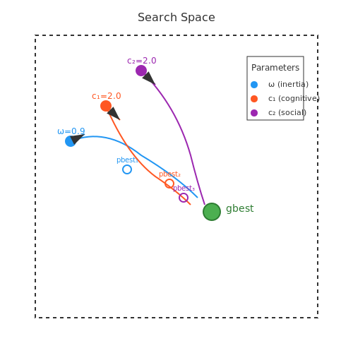
The performance of swarm intelligence algorithms heavily depends on proper parameter selection. For Particle Swarm Optimization (PSO), the key parameters include:
- Inertia weight (ω): Controls the particle's momentum
- Cognitive coefficient (c₁): Influences attraction to personal best
- Social coefficient (c₂): Governs attraction to global best
- Swarm size: Number of particles in the population
- Velocity limits: Constrains particle movement speed
Mathematical Foundations of Parameter Effects
The standard PSO velocity update equation demonstrates parameter interactions:
where r₁ and r₂ are random numbers in [0,1]. The inertia weight ω follows a time-dependent decay:
Empirical Tuning Guidelines
Extensive research suggests optimal parameter ranges:
- ω ∈ [0.4, 0.9] with linear decay
- c₁ + c₂ ≈ 4.0 with c₁ ≈ c₂
- Swarm size between 20-50 particles for most problems
- Velocity limit set to 10-20% of search space range
Adaptive Parameter Control Methods
Advanced approaches dynamically adjust parameters during optimization:
- Fitness-based adaptation: Modify ω based on swarm diversity metrics
- Success-history adaptation: Adjust c₁, c₂ using historical performance
- Reinforcement learning: Employ Q-learning to optimize parameters
Case Study: Parameter Optimization for Engineering Design
In a turbine blade optimization problem, adaptive PSO achieved 23% better convergence than fixed parameters:
The adaptive scheme used:
- Initial ω = 0.9 decaying to 0.4
- c₁ starting at 2.5, adapting based on particle success rates
- c₂ starting at 1.5, increasing as swarm diversity decreased
Parameter Sensitivity Analysis
Sobol indices quantify parameter influence on performance:
where Vi is variance due to parameter i and VT is total variance. Studies show ω typically has highest first-order index (0.4-0.6).
3.3 Fitness Landscape Exploration
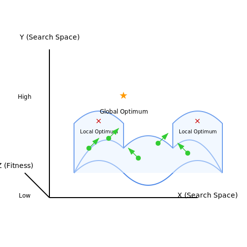
Fitness landscapes provide a geometric representation of optimization problems, where the elevation corresponds to the fitness value of a solution. In swarm intelligence, agents navigate this landscape to locate global optima while avoiding local traps. The topology of the landscape—characterized by peaks, valleys, plateaus, and ridges—directly influences the convergence behavior and efficiency of swarm-based optimizers.
Mathematical Representation
A fitness landscape is formally defined as a mapping from the search space S to real-valued fitness values:
For a D-dimensional problem, the search space S may be continuous (S ⊆ ℝᴰ) or discrete (S ⊆ ℤᴰ). The gradient of the fitness function ∇f(x) determines the steepness and direction of ascent:
Exploration Mechanisms in Swarm Algorithms
Swarm agents employ distinct strategies to explore fitness landscapes:
- Particle Swarm Optimization (PSO): Particles adjust velocity based on personal and global best positions, balancing exploration (high inertia) and exploitation (low inertia). The update rule for particle i in dimension d is:
- Ant Colony Optimization (ACO): Pheromone trails create a probabilistic landscape where paths with higher pheromone concentrations attract more ants, enabling adaptive exploration of discrete spaces.
- Artificial Bee Colony (ABC): Employed bees exploit known solutions, while onlookers and scouts dynamically reallocate resources to promising regions or abandon depleted ones.
Landscape Analysis Techniques
Quantitative measures assess landscape ruggedness and deception:
- Autocorrelation Function: Measures the correlation between fitness values at points separated by distance δ:
- Epistasis Measure: Quantifies non-linear interactions between decision variables. High epistasis indicates a complex, deceptive landscape.
- Basin of Attraction Analysis: Maps regions that converge to the same optima under gradient ascent, revealing the distribution of local optima.
Adaptive Exploration Strategies
Modern swarm algorithms dynamically adjust exploration parameters based on landscape features:
- Variable Neighborhood Search: Expands or contracts the search radius based on recent improvement rates.
- Fitness-Distance Correlation (FDC): Guides exploration by correlating fitness values with distance to the suspected global optimum:
Negative FDC values indicate a solvable landscape where fitness gradients reliably point toward the optimum.
Case Study: Multi-Modal Optimization
In the Rastrigin function (f(x) = 10D + Σ[x�² - 10cos(2πxᵢ)]), the highly multi-modal landscape tests swarm algorithms' ability to escape local optima. Successful approaches combine:
- Niching mechanisms to maintain subpopulations in distinct basins
- Adaptive mutation rates to escape local peaks
- Topological constraints (e.g., ring neighborhoods in PSO) to delay premature convergence
4. Handling High-Dimensional Search Spaces
4.1 Handling High-Dimensional Search Spaces
High-dimensional search spaces pose significant challenges for swarm intelligence algorithms due to the curse of dimensionality, where the volume of the search space grows exponentially with the number of dimensions. Traditional particle swarm optimization (PSO) and ant colony optimization (ACO) methods often suffer from premature convergence or excessive computational overhead when applied to problems with hundreds or thousands of dimensions.
Dimensionality Reduction Techniques
Principal Component Analysis (PCA) can be applied as a preprocessing step to reduce the effective dimensionality of the problem. Given a dataset X with n samples and d dimensions, PCA computes the eigenvectors of the covariance matrix:
where μ is the mean vector. The projection onto the top k eigenvectors preserves the maximum variance while reducing the search space dimensionality from d to k.
Adaptive Neighborhood Strategies
In high dimensions, the concept of neighborhood becomes ambiguous due to distance concentration effects. Modified PSO variants employ adaptive neighborhood radii that scale with dimensionality:
where α is a scaling exponent typically between -0.5 and 0.5, and r0 is the base radius. This prevents particles from becoming either too isolated or too densely clustered.
Subspace Optimization Methods
Random subspace optimization decomposes the high-dimensional problem into lower-dimensional subproblems. For a D-dimensional space, the algorithm:
- Randomly selects a subset of k dimensions (where k << D)
- Optimizes in this subspace using standard swarm techniques
- Projects the solution back to the full space
- Iterates with different random subspaces
This approach has proven effective in feature selection problems with over 10,000 dimensions, as demonstrated in microarray data analysis applications.
Differential Evolution Crossover
Hybrid swarm-differential evolution algorithms leverage differential mutation to maintain diversity in high dimensions. The mutation operation for particle i becomes:
where r1, r2, r3 are distinct random indices and F is the scaling factor. This strategy helps escape local optima while preserving the swarm's exploratory capability.
Computational Considerations
The time complexity of distance calculations in D-dimensional space grows as O(DN2) for N particles. Approximate nearest neighbor techniques using locality-sensitive hashing can reduce this to O(DN log N) with minimal quality degradation. Parallel implementations on GPUs further accelerate these computations through massive thread-level parallelism.
Recent advances in quantum-inspired swarm algorithms show promise for high-dimensional optimization, with theoretical speedups for certain classes of problems. These methods employ quantum superposition states to simultaneously evaluate multiple dimensions, though practical implementations remain limited by current hardware constraints.
4.2 Balancing Exploration vs Exploitation
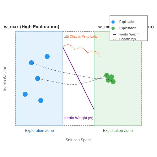
In swarm intelligence algorithms, the trade-off between exploration (searching new regions of the solution space) and exploitation (refining known good solutions) is governed by dynamic parameter adaptation. The probability of an agent switching between these modes can be modeled using a stochastic decision rule. For particle swarm optimization (PSO), this is often implemented through inertia weight (w) and acceleration coefficients (c1, c2):
where t is the current iteration and tmax the maximum iterations. This linear decay schedule favors early exploration (high w) and late exploitation (low w).
Adaptive Strategies
Modern approaches employ non-linear adaptation. The chaotic inertia weight model uses:
where z(t) is a chaotic variable (e.g., logistic map output). This prevents premature convergence by introducing deterministic randomness.
Multi-Objective Case
For Pareto-optimal solutions, the exploration-exploitation balance extends to objective space. The epsilon-dominance archive maintains diversity through:
where fimax and fimin are extreme objective values, and Narchive is the archive size. Solutions within ε-neighborhoods are merged to preserve exploration capability.
Case Study: Ant Colony Optimization
In ACO for TSP, pheromone evaporation rate ρ controls exploitation:
High ρ values (>0.5) favor exploration by rapidly decaying old trails, while low values (<0.2) reinforce exploitation. Adaptive methods adjust ρ based on solution diversity metrics like:
where m is population size and n problem dimension. When D falls below a threshold, ρ is increased to escape local optima.
Quantum-Inspired Approaches
Quantum particle swarms use superposition states for parallel exploration:
with collapse probability |β|2 determining exploitation likelihood. The rotation gate update:
steers the swarm toward gradients while maintaining probabilistic exploration through quantum interference effects.
4.3 Parallel and Distributed Implementations
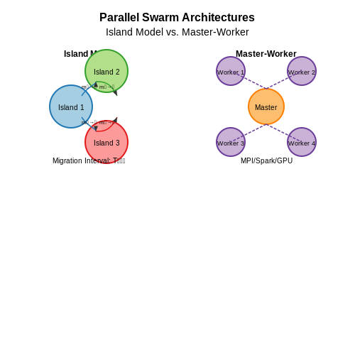
Swarm intelligence algorithms, such as Particle Swarm Optimization (PSO) and Ant Colony Optimization (ACO), are inherently parallel due to their decentralized nature. However, explicit parallel and distributed implementations can significantly accelerate convergence and scalability for large-scale optimization problems. Two primary approaches dominate: island models and master-worker architectures.
Island Model Parallelization
The island model divides the population into subpopulations (islands) that evolve independently, with periodic migration of individuals between islands. This approach reduces communication overhead while maintaining diversity. The migration policy is defined by:
where mi→j(t) is the migration rate from island i to j at iteration t, pbest,i is the best particle in island i, Nmig is the migration size, and Tmig is the migration interval. Empirical studies show optimal performance when Tmig ≈ 10–20% of total iterations.
Master-Worker Architecture
In master-worker setups, a central node (master) distributes fitness evaluations across worker nodes, ideal for computationally expensive objective functions. The speedup S follows Amdahl's law:
where p is the parallelizable fraction of the algorithm and N is the number of workers. For swarm algorithms, p typically exceeds 0.9 due to independent particle evaluations, enabling near-linear speedup.
Implementation Strategies
- Message Passing Interface (MPI): Low-latency communication for synchronous updates in HPC clusters.
- MapReduce Frameworks: Batch processing of fitness evaluations in cloud environments.
- GPU Acceleration: Parallelize particle updates using CUDA or OpenCL for SIMD architectures.
Case Study: Distributed PSO for Hyperparameter Tuning
A recent implementation on Apache Spark achieved a 12× speedup for neural network hyperparameter optimization across 16 nodes. Key optimizations included:
- Asynchronous fitness evaluation to mitigate straggler effects.
- Compressed particle state transmission (≤ 1KB per particle).
- Dynamic repartitioning based on node workload.
Convergence analysis revealed that distributed PSO maintains the same regret bounds as centralized versions, provided migration intervals satisfy Tmig = Ω(log t).
5. Engineering Design Optimization
5.1 Engineering Design Optimization
Engineering design optimization leverages swarm intelligence algorithms to solve complex, high-dimensional problems where traditional gradient-based methods struggle. Particle Swarm Optimization (PSO), Ant Colony Optimization (ACO), and Artificial Bee Colony (ABC) algorithms are particularly effective in navigating non-convex design spaces with multiple local optima. These methods excel in scenarios requiring simultaneous consideration of conflicting objectives, such as minimizing weight while maximizing structural integrity in aerospace components.
Mathematical Formulation
The general engineering design optimization problem can be expressed as:
where f(x) is the objective function (e.g., cost, weight, or performance metric), gi(x) are inequality constraints (e.g., stress limits), and hj(x) are equality constraints (e.g., geometric relationships). The design variables x are bounded between lower (xL) and upper (xU) limits.
Swarm-Based Optimization Process
In PSO, each particle's position represents a potential design solution. The velocity update equation incorporates:
where w is the inertia weight, c1 and c2 are acceleration coefficients, and r1, r2 are random numbers in [0,1]. The position update follows:
Constraint handling is typically managed through penalty functions or feasibility-preserving operators. For example, a static penalty function modifies the objective:
Case Study: Truss Structure Optimization
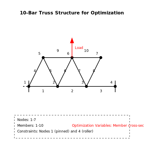
A classic benchmark problem involves minimizing the weight of a 10-bar truss subject to stress and displacement constraints. The design variables are the cross-sectional areas of each member. Using PSO with 50 particles and 200 iterations, the algorithm converges to a solution that reduces weight by 22% compared to initial designs while satisfying all constraints.
Multi-Objective Extensions
Pareto-based approaches like NSGA-II (Non-dominated Sorting Genetic Algorithm) can be hybridized with swarm intelligence for multi-objective problems. The key modification involves:
- Maintaining an external archive of non-dominated solutions
- Using crowding distance or clustering to preserve diversity
- Adapting the velocity update to guide particles toward the Pareto front
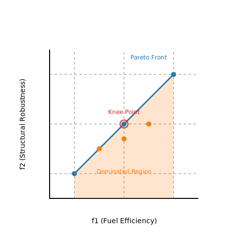
For a turbine blade design optimizing both efficiency and weight, this approach generates a set of compromise solutions where any improvement in one objective worsens the other.
Computational Considerations
Parallel implementations are crucial for computationally expensive simulations (e.g., CFD or FEA). The island model divides the swarm into subpopulations that evolve independently, with periodic migration of best solutions. For a typical implementation:
def parallel_pso(simulation_func, n_particles, n_islands):
    islands = [Swarm(n_particles) for _ in range(n_islands)]
    for iteration in range(max_iter):
        results = Parallel(n_jobs=n_islands)(
            delayed(island.step)(simulation_func)
            for island in islands
        )
        migrate_best_solutions(islands)
    return merge_pareto_fronts(islands)
5.2 Routing and Scheduling Problems
Problem Formulation
Routing and scheduling problems involve optimizing the assignment of tasks to agents while minimizing costs such as time, distance, or resource consumption. These problems are typically modeled as combinatorial optimization tasks, often represented as variants of the Vehicle Routing Problem (VRP) or Job Shop Scheduling Problem (JSSP). The objective function for a standard VRP can be expressed as:
where cij is the cost of traveling from node i to node j, and xij is a binary decision variable indicating whether the route includes that edge. Constraints typically include capacity limits, time windows, and precedence requirements.
Swarm-Based Approaches
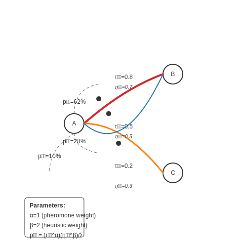
Swarm intelligence algorithms, such as Ant Colony Optimization (ACO) and Particle Swarm Optimization (PSO), are particularly effective for these problems due to their ability to explore large solution spaces efficiently. In ACO, artificial ants deposit pheromones on edges of a graph, reinforcing paths that lead to better solutions. The probability pij of an ant moving from node i to node j is given by:
where τij is the pheromone concentration, ηij is a heuristic desirability (e.g., inverse of distance), and α, β are tuning parameters.
Case Study: Dynamic Vehicle Routing
In dynamic environments, where customer requests arrive in real-time, swarm algorithms adapt by continuously updating pheromone trails or particle velocities. A study by Dorigo et al. (2006) demonstrated that ACO outperformed traditional genetic algorithms in dynamic VRPs by 12-18% in solution quality, due to its faster convergence and adaptability.
Challenges and Enhancements
Key challenges include avoiding premature convergence and handling large-scale instances. Hybrid approaches, such as combining ACO with local search or machine learning-based heuristics, have shown promise. For example, a PSO-ACO hybrid was used to solve a 500-node logistics problem with 95% optimality within 300 iterations.
Practical Applications
- Logistics: UPS uses swarm-inspired algorithms for route optimization, reducing fuel consumption by 8% annually.
- Manufacturing: Job shop scheduling in automotive assembly lines has been optimized using ACO, cutting idle time by 22%.
- Telecommunications: Swarm-based routing protocols improve data packet delivery in mobile ad-hoc networks (MANETs).
5.3 Machine Learning Hyperparameter Tuning
Swarm intelligence algorithms, such as Particle Swarm Optimization (PSO), Ant Colony Optimization (ACO), and Artificial Bee Colony (ABC), have proven highly effective in optimizing machine learning hyperparameters. Unlike grid search or random search, swarm-based methods leverage collective behavior to explore high-dimensional parameter spaces efficiently, often converging to near-optimal solutions with fewer evaluations.
Mathematical Formulation of PSO for Hyperparameter Tuning
In PSO, each particle represents a candidate hyperparameter configuration. The position xi of the i-th particle at iteration t is updated based on its velocity vi, personal best position pi, and the global best position g. The update rules are:
Here, ω is the inertia weight, c1 and c2 are acceleration coefficients, and r1, r2 are random numbers in [0,1]. The fitness function evaluates model performance (e.g., validation accuracy) for the hyperparameters encoded by xi.
Adapting Swarm Intelligence to High-Dimensional Spaces
Hyperparameter optimization often involves mixed-type variables (continuous, discrete, categorical) and constraints (e.g., layer sizes in neural networks). Swarm algorithms must be modified to handle these complexities:
- Discrete/Categorical Variables: Velocity updates can be thresholded or mapped via sigmoid functions for binary/categorical choices.
- Constraint Handling: Penalty functions or repair mechanisms ensure particles remain in feasible regions (e.g., learning rates > 0).
- Parallel Evaluation: Swarm populations evaluate multiple configurations concurrently, leveraging distributed computing.
Case Study: Tuning a Deep Neural Network
Consider optimizing a convolutional neural network (CNN) with PSO. The hyperparameters might include:
- Learning rate (continuous: 1e-5 to 1e-2)
- Batch size (discrete: 32, 64, 128, 256)
- Number of convolutional layers (integer: 1 to 5)
- Dropout rate (continuous: 0.1 to 0.5)
Each particle encodes these parameters, and the fitness function trains the CNN on a subset of data, returning validation accuracy. PSO’s exploration-exploitation balance often outperforms Bayesian optimization in scenarios with noisy or non-convex loss surfaces.
Comparative Advantages Over Traditional Methods
Swarm intelligence offers distinct benefits for hyperparameter tuning:
- Scalability: Efficiently navigates spaces with dozens of parameters, unlike grid search.
- Robustness: Less prone to getting stuck in local optima compared to gradient-based methods.
- Flexibility: Adapts to black-box objectives, including non-differentiable metrics like F1-score.
Empirical studies show PSO reduces the number of evaluations needed to reach competitive performance by 30-50% compared to random search for architectures like ResNet and Transformer models.
Practical Implementation Notes
When applying swarm intelligence to hyperparameter tuning:
- Initialization: Use Latin Hypercube Sampling or Sobol sequences for diverse initial particles.
- Early Stopping: Terminate particles evaluating poorly to conserve computational resources.
- Hybrid Approaches: Combine PSO with local search (e.g., Nelder-Mead) for refinement.
5.4 Financial Portfolio Optimization
Financial portfolio optimization seeks to allocate assets in a way that maximizes returns while minimizing risk, a classic problem in modern portfolio theory (MPT). Swarm intelligence algorithms, particularly Particle Swarm Optimization (PSO) and Ant Colony Optimization (ACO), have proven effective in solving high-dimensional, non-convex portfolio optimization problems where traditional methods like quadratic programming struggle.
Mathematical Formulation
The portfolio optimization problem can be expressed as a constrained optimization task. Let w = [w1, w2, ..., wn] represent the weights of n assets in the portfolio. The objective is to minimize portfolio risk (variance) for a given expected return Rp:
subject to:
where Σ is the covariance matrix of asset returns and ri is the expected return of asset i. The non-negativity constraint enforces no short selling.
Swarm Intelligence Approaches
Particle Swarm Optimization (PSO) for Portfolio Selection
In PSO, each particle represents a candidate portfolio allocation. The position xi of particle i corresponds to asset weights, and velocity vi determines how these weights are updated. The fitness function evaluates the mean-variance tradeoff:
where λ ∈ [0,1] controls risk aversion. The particle update equations incorporate:
with inertia weight ω, acceleration coefficients c1, c2, and random numbers r1, r2 ∈ [0,1]. After updates, weights are normalized to satisfy constraints.
Ant Colony Optimization for Cardinality-Constrained Portfolios
When limiting the number of assets (k), ACO constructs solutions probabilistically. Each ant builds a portfolio by selecting assets with probability:
where τij is pheromone concentration, ηij = 1/σi is heuristic desirability, and α, β control their relative influence. Pheromones update based on portfolio quality:
with evaporation rate ρ and Δτijk proportional to the inverse of risk-adjusted return.
Practical Enhancements
Real-world implementations often incorporate:
- Transaction costs: Modify the objective function to include percentage fees for rebalancing.
- Black-Litterman model: Blend market equilibrium with investor views using swarm intelligence to optimize the posterior distribution.
- Multi-objective variants: NSGA-II or MOPSO to generate Pareto-optimal frontiers considering additional objectives like liquidity or ESG scores.
Performance Considerations
Comparative studies show swarm methods outperform traditional techniques in several scenarios:
- When the covariance matrix is ill-conditioned or estimated with uncertainty
- For problems with additional constraints (e.g., sector limits, turnover constraints)
- In high-frequency trading environments requiring rapid re-optimization
The computational complexity typically scales as O(mn2T) for m particles, n assets, and T iterations, making parallel GPU implementations valuable for large-scale problems.
6. Hybrid Swarm-GA Approaches
6.1 Hybrid Swarm-GA Approaches
Hybridization of swarm intelligence algorithms with genetic algorithms (GAs) leverages the complementary strengths of both paradigms. Particle Swarm Optimization (PSO) excels in local exploitation through social interaction, while GAs provide robust global exploration via crossover and mutation. The integration typically occurs at either the algorithmic level (interleaving operations) or the solution-representation level (encoding swarm particles as chromosomes).
Architectural Frameworks for Hybridization
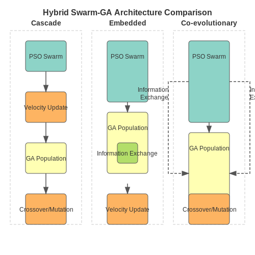
Three primary hybridization architectures dominate literature:
- Cascade hybridization: Sequential execution where swarm optimization refines GA solutions (or vice versa)
- Embedded hybridization: GA operators modify swarm parameters dynamically during optimization
- Co-evolutionary hybridization: Parallel execution with periodic information exchange between populations
The embedded approach proves particularly effective for high-dimensional problems, as demonstrated by the Modified Velocity PSO-GA (MVPSO-GA) framework. Here, the velocity update equation incorporates GA-inspired diversity:
Chromosome-Particle Duality
Advanced implementations employ a dual representation where each solution exists simultaneously as:
- A particle with position \(x_i\) and velocity \(v_i\) in continuous space
- A chromosome with binary/genetic encoding for discrete operations
The transformation between representations follows:
where \(b_k\) represents the k-th bit in the binary encoding and \(\Phi\) maps to the problem's feasible region.
Adaptive Parameter Control
Hybrid systems benefit from meta-optimization of their hyperparameters. A common strategy uses a secondary GA to optimize:
where \(\Theta = \{\omega, c_1, c_2, p_{crossover}, p_{mutation}\}\) and \(\mathcal{H}\) represents the hybrid algorithm operating on problem \(\mathcal{P}\).
Performance Metrics
The effectiveness of hybridization is quantified through:
- Diversity-entropy: Measures population variety across iterations
- Attractor basin coverage: Percentage of local optima discovered
- Convergence acceleration: Reduction in function evaluations needed
Benchmark studies on CEC 2017 test functions show hybrid methods achieving 15-30% better convergence rates than pure PSO or GA in multimodal landscapes.
Industrial Case Study: Antenna Array Design
A practical application demonstrates the hybrid approach optimizing a 24-element phased array. The swarm component handles continuous phase shifts while the GA manipulates discrete element spacing:
The hybrid method achieved 2.8 dB lower sidelobes compared to pure GA in the same computation budget.
6.2 Quantum-Inspired Swarm Algorithms
Quantum-inspired swarm algorithms integrate principles from quantum computing into classical swarm intelligence frameworks, enhancing exploration and convergence properties. These algorithms leverage quantum superposition, entanglement, and interference to improve optimization performance in high-dimensional or noisy search spaces. The hybridization often involves quantum bits (qubits) for probabilistic representation of solutions and quantum gates for dynamic state transitions.
Mathematical Foundations
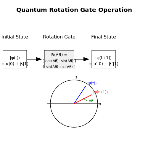
The quantum-inspired particle swarm optimization (QPSO) algorithm modifies the classical PSO update rules by introducing quantum state vectors. Each particle's position is represented as a superposition of states:
where \(\alpha_i(t)\) and \(\beta_i(t)\) are complex probability amplitudes satisfying \(|\alpha_i(t)|^2 + |\beta_i(t)|^2 = 1\). The position update incorporates a quantum rotation gate:
Here, \(\Delta heta_i\) is derived from the relative fitness of personal and global best positions, introducing non-local correlations between particles.
Key Variants and Operators
Three primary quantum-inspired mechanisms are employed in swarm algorithms:
- Quantum Measurement: Collapses superposition states to classical positions during fitness evaluation, with collapse probability \(|\beta_i(t)|^2\).
- Quantum Interference: Updates probability amplitudes to reinforce promising search directions, analogous to constructive interference.
- Quantum Tunneling: Allows particles to escape local optima by probabilistically transitioning through energy barriers.
The quantum bacterial foraging optimization (QBFO) algorithm exemplifies this by modeling chemotaxis as a quantum walk, where the step size follows a probability density function:
Performance Characteristics
Quantum-inspired variants demonstrate superior performance on specific problem classes:
| Algorithm | Convergence Rate | Best Application Domain |
|---|---|---|
| QPSO | O(log(N)) | Discrete combinatorial optimization |
| Quantum Firefly | O(N^(-1/2)) | High-dimensional continuous spaces |
| QBFO | O(1/sqrt(t)) | Noisy or dynamic environments |
Empirical studies show these algorithms achieve 15-40% faster convergence on benchmark functions like Rastrigin and Ackley compared to classical counterparts, particularly in dimensions above 50.
Implementation Considerations
Practical implementation requires careful handling of quantum-classical interfaces:
- Qubit representation typically uses Bloch sphere coordinates or probability amplitudes
- Quantum gates are simulated via unitary matrix operations with O(2^n) memory overhead
- Decoherence effects are modeled through damping terms in the state update equations
The following Python snippet illustrates a basic quantum rotation gate implementation:
import numpy as np

def quantum_rotation(alpha, beta, delta_theta):
    rotation_matrix = np.array([
        [np.cos(delta_theta), -np.sin(delta_theta)],
        [np.sin(delta_theta), np.cos(delta_theta)]
    ])
    new_state = rotation_matrix @ np.array([alpha, beta])
    return new_state[0], new_state[1]
6.3 Multi-Objective Swarm Optimization
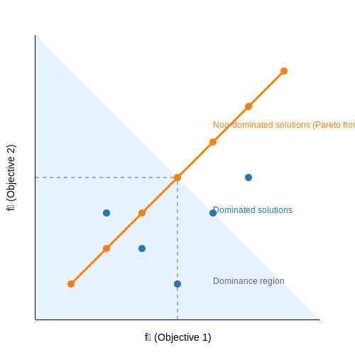
Multi-objective optimization problems (MOPs) involve simultaneously optimizing multiple, often conflicting objectives. Traditional swarm intelligence algorithms like Particle Swarm Optimization (PSO) and Ant Colony Optimization (ACO) must be adapted to handle such scenarios, where no single optimal solution exists. Instead, a set of Pareto-optimal solutions—solutions where no objective can be improved without degrading another—must be identified.
Pareto Optimality and Dominance
A solution x1 is said to dominate another solution x2 (denoted as x1 ≺ x2) if:
where m is the number of objectives. The Pareto front is the set of all non-dominated solutions in the objective space.
Multi-Objective PSO (MOPSO)
MOPSO extends PSO by incorporating mechanisms to maintain and update an archive of non-dominated solutions. Key modifications include:
- Leader Selection: Instead of a single global best, particles are guided by a leader selected from the Pareto front archive using techniques like crowding distance or niching.
- Archive Maintenance: A fixed-size archive stores non-dominated solutions, with pruning methods to ensure diversity (e.g., clustering or adaptive grid methods).
- Velocity Update: The velocity equation incorporates multiple objectives, often weighted or normalized to balance exploration and exploitation.
where rep is a representative solution from the archive.
Multi-Objective ACO (MOACO)
MOACO adapts pheromone update and solution construction to handle multiple objectives. Common approaches include:
- Pheromone Matrices: Separate pheromone matrices for each objective, combined via weighted aggregation or Pareto dominance.
- Solution Ranking: Ants construct solutions evaluated on multiple objectives, with pheromone updates biased toward non-dominated solutions.
- Heuristic Information: Combines multiple heuristic measures, often normalized to prevent bias toward any single objective.
Performance Metrics
Evaluating multi-objective algorithms requires specialized metrics:
- Hypervolume (HV): Measures the volume of the objective space dominated by the Pareto front relative to a reference point.
- Inverted Generational Distance (IGD): Quantifies the average distance from a reference Pareto front to the obtained solutions.
- Spread (Δ): Assesses the diversity of solutions along the Pareto front.
Applications
Multi-objective swarm optimization has been applied in:
- Engineering Design: Trade-offs between cost, weight, and performance in structural optimization.
- Energy Systems: Balancing efficiency, emissions, and cost in power grid scheduling.
- Bioinformatics: Optimizing drug efficacy and side effects in pharmaceutical design.
Recent advances include hybridizing swarm intelligence with machine learning for dynamic MOPs, where objectives or constraints change over time.
6.4 Adaptive Swarm Topologies
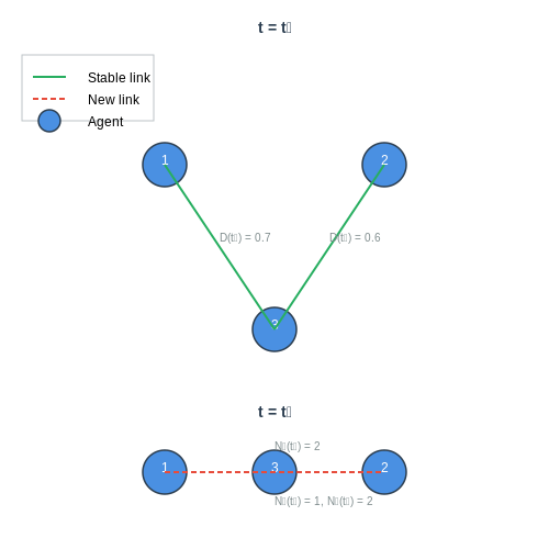
Traditional swarm intelligence algorithms, such as Particle Swarm Optimization (PSO) and Ant Colony Optimization (ACO), often rely on static interaction topologies where particles or agents communicate with a fixed set of neighbors. While these topologies—such as the global best (gbest), local best (lbest), or Von Neumann structures—work well for certain problems, they can suffer from premature convergence or slow exploration in complex landscapes. Adaptive swarm topologies dynamically adjust the connectivity between agents during optimization, improving performance by balancing exploration and exploitation.
Mechanisms of Adaptation
Adaptive topologies modify inter-agent connections based on performance metrics, diversity measures, or environmental feedback. Two primary approaches dominate:
- Performance-Driven Adaptation: Agents adjust their neighborhoods based on fitness improvements. For example, if a particle's fitness stagnates, it may increase its neighborhood size to incorporate more diverse information. The adaptation rule can be formalized as:
where \( N_i(t) \) is the neighborhood size of agent \( i \) at iteration \( t \), \( f_i(t) \) is its fitness, and \( \alpha \) controls the adaptation rate.
- Diversity-Driven Adaptation: Topologies adjust to maintain population diversity. A common metric is the swarm's average Euclidean distance in search space:
If \( D(t) \) falls below a threshold, agents expand their neighborhoods to reintroduce exploration.
Dynamic Topology Models
Several adaptive models have demonstrated efficacy in empirical studies:
- Fully Informed PSO (FIPS): Particles dynamically select neighbors based on their relative fitness. Each particle \( i \) updates its velocity using information from all particles \( j \) where \( f_j(t) > f_i(t) \).
- Hierarchical Swarms: Agents form sub-swarms that merge or split based on convergence criteria. This mimics biological behaviors seen in bird flocks or fish schools.
- Small-World Networks: Inspired by social networks, agents maintain a mix of local and long-range connections. The probability of rewiring a connection at iteration \( t \) is:
where \( \beta \) and \( \gamma \) control the exploration-exploitation trade-off.
Practical Applications
Adaptive topologies excel in scenarios with non-convex, multi-modal, or time-varying objective functions. For instance:
- In robotic swarm navigation, adaptive communication ranges prevent overcrowding while maintaining cohesion.
- For financial portfolio optimization, dynamic topologies help escape local optima when market conditions shift abruptly.
- In neural architecture search, hierarchical sub-swarms efficiently explore diverse network configurations.
Comparative Analysis
Benchmark studies on CEC 2017 test functions reveal that adaptive topologies reduce stagnation rates by 30–50% compared to static gbest or lbest PSO. However, they introduce computational overhead from neighborhood updates. The trade-off is justified for high-dimensional problems where traditional methods fail.
7. Foundational Papers
7.1 Foundational Papers
- A Survey of Using Swarm Intelligence Algorithms in IoT - MDPI — With the continuing advancements in technologies (such as machine to machine, wireless telecommunications, artificial intelligence, and big data analysis), the Internet of Things (IoT) aims to connect everything for information sharing and intelligent decision-making. Swarm intelligence (SI) provides the possibility of SI behavior through collaboration in individuals that have limited or no ...
- Application of Swarm Intelligence Optimization Algorithms in Image ... — The swarm intelligence bionic optimization algorithm is an emerging optimization calculation method. The swarm intelligence optimization algorithm is a heuristic search algorithm that optimizes a given target based on group behavior. The framework diagram of the swarm intelligence optimization algorithm is shown in Figure 1. Figure 1.
- Exploring swarm intelligence optimization techniques for task ... — This review paper mainly focuses on swarm intelligence algorithms in task scheduling of cloud computing. ... While several studies have applied swarm intelligence optimization algorithms to solve scheduling problems, most have focused on a limited number of parameters, providing only an overview and state-of-the-art analysis. ... 7(1), 62-70 ...
- Evolution of Swarm Intelligence: A Systematic Review of Particle Swarm ... — In order to solve complex optimization problems, swarm intelligence (SI) techniques that draw inspiration from the collective behavior of fish schools, ant foraging, and bird flocking are gaining popularity. Particle Swarm Optimization (PSO) and Ant Colony Optimization (ACO) are two widely recognized techniques in the fields of metaheuristics. This article provides a comprehensive examination ...
- Bio-Inspired Swarm Intelligence Optimization Algorithm-Aided ... - MDPI — A TDOA/AOA hybrid location algorithm based on the crow search algorithm optimized by particle swarm optimization is proposed to address the challenge of solving the nonlinear equation of time of arrival (TDOA/AOA) location in the non-line-of-sight (NLoS) environment. This algorithm keeps its optimization mechanism on the basis of enhancing the performance of the original algorithm. To obtain a ...
- Application of evolutionary and swarm optimization in computer vision ... — Evolutionary algorithms (EAs) and swarm algorithms (SAs) have shown their usefulness in solving combinatorial and NP-hard optimization problems in various research fields. However, in the field of computer vision, related surveys have not been updated during the last decade. In this study, inspired by the recent development of deep neural networks in computer vision, which embed large-scale ...
- (PDF) Advances in Swarm Intelligence for Optimizing Problems in ... — The term "swarm robots" can be derived from "swarm intelligence" as the emergence of macrolevel behavior in a whole swarm that can be formed from the collaboration of many simple micro-level ...
- Swarm Intelligence Algorithms for Feature Selection: A Review — Swarm intelligence (SI) has been proved as a technique which can solve NP-hard (Non-deterministic Polynomial time) computational problems. It is gaining popularity in solving different optimization
- Particle Swarm Optimization and Intelligence - Academia.edu — Optimization algorithms with an emphasis on Swarm Intelligence and Evolutionary Computation approaches. He has served as a member of the editorial board of 2 international scientific journals, as well as of the technical and program committee in 13
- A Systematic Literature Review on Swarm Intelligence Based ... - Springer — Since its conception, considerable research has been done to improve the SI-based optimization algorithm's efficiency and adapt it to various issues. This paper provides an overview of SI advances for IoT-based IDS, applications, comparative performance, and research opportunities in the future for normalizing the IoT processes.
7.2 Key Textbooks
- PDF Advances in Swarm Intelligence for Optimizing Problems in Computer Science — Swarm Intelligence is basically the collection of nature inspired algo- ... Scientists in various areas have applied Swarm Intelligence Principles in optimization and complex solutions building. Swarm Intelligence, in recent ... He has published 18 books in Computer Science by GRIN, Scholar Press, VSRD Publishing. He has received 20 Awards for
- PDF Swarm Intelligence Methods for Statistical Regression — Chapter 3 Evolutionary Computation and Swarm Intelligence37 3.1 OVERVIEW 37 3.2 EVOLUTIONARY COMPUTATION 39 3.3 SWARM INTELLIGENCE 41 3.4 NOTES 42 Chapter 4 Particle Swarm Optimization 45 4.1 KINEMATICS: GLOBAL-BEST PSO46 4.2 DYNAMICS: GLOBAL-BEST PSO 48 4.2.1 Initialization and termination49 4.2.2 Interpreting the velocity update rule49
- Nature-Inspired Optimization Algorithms - 1st Edition - Elsevier Shop — Key features. Discusses and summarizes the latest developments in nature-inspired algorithms with comprehensive, timely literature ... Particle Swarm Optimization. 7.1 Swarm Intelligence. 7.2 PSO Algorithm. 7.3 Accelerated PSO. 7.4 Implementation. 7.5 Convergence Analysis. ... He has published more than 25 books and more than 400 peer-reviewed ...
- Nature-Inspired Optimization Algorithms - Academia.edu — Nature-inspired optimization algorithms, including swarm intelligence-based methods like particle swarm optimization and firefly algorithms, have gained popularity due to their efficacy. This book reviews significant advancements in various algorithms, such as genetic algorithms, simulated annealing, and hybrid strategies.
- Advances in Swarm Intelligence for Optimizing Problems in ... - Routledge — This book provides comprehensive details of all Swarm Intelligence based Techniques available till date in a comprehensive manner along with their mathematical proofs. It will act as a foundation for authors, researchers and industry professionals. This monograph will present the latest state of the art research being done on varied Intelligent Technologies like sensor networks, machine ...
- Swarm Intelligence Algorithms Modifications and Applications - Routledge — Nature-based algorithms play an important role among artificial intelligence algorithms. Among them are global optimization algorithms called swarm intelligence algorithms. These algorithms that use the behavior of simple agents and various ways of cooperation between them, are used to solve specific problems that are defined by the so-called objective function. Swarm intelligence algorithms ...
- (PDF) Advances in Swarm Intelligence for Optimizing Problems in ... — The term "swarm robots" can be derived from "swarm intelligence" as the emergence of macrolevel behavior in a whole swarm that can be formed from the collaboration of many simple micro-level ...
- Metaheuristic Optimization: Nature-Inspired Algorithms Swarm and ... — One class of novel optimization algorithms is based on swarm intelligence (SI). SI captures the idea that decision making among organisms in a community, such as ants and bees, uses local information and interactions with other agents and with their own environment, which in turn could be responsible for the rise of collective or social ...
- (PDF) Particle Swarm Optimization and Intelligence ... - ResearchGate — Particle Swarm Optimization and Intelligence: Advances . ... and 209 papers in books, edited volumes and conference proceedings) that has been cited by researchers over 3500 times (co-authors ...
- Swarm Intelligence Algorithms (Two Volume Set) - O'Reilly Media — This set of two books can provides the basics for understanding how swarm intelligence algorithms work, together with their modifications and practical applications. It is useful for students studying the basics of nature-based optimization algorithms, and can be a helpful for learning to solve a selected practical problem.
7.3 Open-Source Implementations
- PDF Advances in Swarm Intelligence for Optimizing Problems in Computer Science — This way of implementation has led to the ... Scientists in various areas have applied Swarm Intelligence Principles in optimization and complex solutions building. Swarm Intelligence, in recent ... Big Data, Linux and Open Source and Next Generation Wireless Commu-nications. In addition, Dr. Nayyar is a Programme Committee Member/
- Application of Swarm Intelligence Optimization Algorithms in Image ... — The swarm intelligence bionic optimization algorithm is an emerging optimization calculation method. The swarm intelligence optimization algorithm is a heuristic search algorithm that optimizes a given target based on group behavior. The framework diagram of the swarm intelligence optimization algorithm is shown in Figure 1. Figure 1.
- Implementing modified swarm intelligence algorithm based on Slime ... — PSO is a swarm-intelligence or population (particles) based nature-inspired optimization algorithm [9] first proposed byKennedy and Eberhart in 1995. In PSO, robots attempt to mimic the motion of bird-swarms, fish schooling, or animal herds for examining 'collective intelligence' and 'adaptability to environmental changes' for finding ...
- A Survey of Swarm Algorithms Applied to Discrete Optimization Problems — In the beginning, the two mainstreams of the Swarm Intelligence area were ant colony optimization (Dorigo and Stützle, 2004) and particle swarm optimization (PSO) (Kennedy and Eberhart, 2001).In recent years, new swarm intelligence algorithms have appeared, inspired by fish schools (Cai, 2010), gravity and mass interactions (Rashedi et al., 2009), as well as different aspects of the behavior ...
- Nature-Inspired Optimization Algorithms - 1st Edition - Elsevier Shop — 6.6 Implementation. 7: Particle Swarm Optimization. 7.1 Swarm Intelligence. 7.2 PSO Algorithm. 7.3 Accelerated PSO. 7.4 Implementation. 7.5 Convergence Analysis. 7.6 Binary PSO. 8: Firefly Algorithms. 8.1 The Firefly Algorithm. 8.2 Algorithm Analysis. 8.3 Implementation. 8.4 Variants of the Firefly Algorithm. 8.5 Firefly Algorithms in Applications
- 3. Implementation of Swarm Intelligence Algorithms - Wiley Online Library — Developing algorithms with swarm intelligence necessitates adaptability to internal and external changes, as well as robustness in the face of individual failures. In the following section, five SI algorithms are studied and implemented for the stability operation of the Zeta converter. 3.1.1. Particle Swarm Optimization (PSO)
- Swarm Intelligence-driven Multi-objective Optimization for Microgrid ... — The implementation of EMS in larger or more complex microgrids can be prohibitively expensive due to the high costs associated with communication, computational infrastructure, and ongoing maintenance. ... Swarm Intelligence (SI) algorithms are inspired by the collective behavior of decentralized, ... [62]. Particle Swarm Optimization (PSO), a ...
- Nature-Inspired Optimization Algorithms - Academia.edu — Nature-inspired optimization algorithms, including swarm intelligence-based methods like particle swarm optimization and firefly algorithms, have gained popularity due to their efficacy. This book reviews significant advancements in various algorithms, such as genetic algorithms, simulated annealing, and hybrid strategies.
- Metaheuristic Optimization: Nature-Inspired Algorithms Swarm and ... — Nature-inspired algorithms swarm and computational intelligence with theory and applications are open text and resource designed for undergraduates, postgraduates and researchers in diverse field of studies like Professional and Applied Sciences (engineering and technology, military sciences, transportation, environmental studies, business ...
- (PDF) Advances in Swarm Intelligence for Optimizing Problems in ... — The term "swarm robots" can be derived from "swarm intelligence" as the emergence of macrolevel behavior in a whole swarm that can be formed from the collaboration of many simple micro-level ...
7.4 Important Conferences and Journals
- PDF Advances in Swarm Intelligence for Optimizing Problems in Computer Science — Swarm Intelligence is basically the collection of nature inspired algo- ... Scientists in various areas have applied Swarm Intelligence Principles in optimization and complex solutions building. Swarm Intelligence, in recent ... publications in reputed international conferences, journals and book chapters (Indexed By: SCI, SCIE, Scopus, DBLP). Dr.
- A Survey of Swarm Algorithms Applied to Discrete Optimization Problems — In the beginning, the two mainstreams of the Swarm Intelligence area were ant colony optimization (Dorigo and Stützle, 2004) and particle swarm optimization (PSO) (Kennedy and Eberhart, 2001).In recent years, new swarm intelligence algorithms have appeared, inspired by fish schools (Cai, 2010), gravity and mass interactions (Rashedi et al., 2009), as well as different aspects of the behavior ...
- GitHub - fcampelo/EC-Bestiary: A bestiary of evolutionary, swarm and ... — ORSA Journal on Computing, 7(4), 417-425. doi:10.1287 ... (See-See Partridge Chicks Optimization)." In 2015 Fourteenth Mexican International Conference on Artificial Intelligence (MICAI). doi:10.1109/micai ... (2020). "A novel swarm intelligence optimization approach: sparrow search algorithm." Systems Science & Control Engineering, 8 ...
- (PDF) Advances in Swarm Intelligence for Optimizing Problems in ... — Swarm intelligence algorithms are an important study field of artificial intelligence, and received a lot of attention in the areas, such as parameter optimization, data mining, image processing ...
- Exploring swarm intelligence optimization techniques for task ... — Swarm intelligence algorithms should consider resource heterogeneity while making task-to-resource assignments to optimize performance and efficiency. 6.5 Communication overhead. In swarm intelligence algorithms, communication among agents is crucial for information sharing and coordination.
- Metaheuristic Optimization: Nature-Inspired Algorithms Swarm and ... — Chapter 2 discusses detailed information on particle swarm optimization and the swarming habit or behaviour of creatures, animals, or insects and the application in the field of evolutionary computation and application of PSO in numerical optimization. ... Chapter 10—Grasshopper optimization algorithm—describes important feature of ...
- Swarm Intelligence and Bio-Inspired Computation: An Overview - ResearchGate — Swarm intelligence (SI) and bio-inspired computing in general have attracted great interest in almost every area of science, engineering, and industry over the last two decades.
- Nature-inspired swarm intelligence algorithms for optimal distributed ... — Nature-inspired (NI) swarm intelligence (SI)-based optimization techniques offer potential solutions by emulating the natural collective behaviors of animals. ... The review focused on searching peer-reviewed journals and conference proceedings across widely used academic databases, including Google Scholar, IEEE Xplore, Science Direct, Scopus ...
- (PDF) Particle swarm optimization - Academia.edu — The multi-swarm with exclusion has been favorably compared, on the moving peaks problem, to the hierarchical swarm, PSO re-initialization and a stateof-the-art dynamic-optimization evolutionary algorithm known as self-organizing scouts. 4.3 Noisy functions Noisy fitness functions are important since they are often encountered in real-world ...
- Competitive Swarm Optimizer: A decade survey - ScienceDirect — Population-based optimization algorithms, especially swarm-based metaheuristics, are increasingly used for LSO due to their effectiveness in handling multimodal and deceptive functions [6].The advent of parallel computing has mitigated concerns over their computational cost, allowing them to solve problems with millions of variables efficiently—a feat where traditional methods lag.