Multimeters
1. Definition and Purpose of Multimeters
Definition and Purpose of Multimeters
A multimeter is an electronic measuring instrument that combines several measurement functions into a single unit, typically capable of measuring voltage, current, and resistance. Advanced models may also include capacitance, inductance, frequency, temperature, and continuity testing. The device operates by converting analog signals into digital representations through an analog-to-digital converter (ADC), enabling precise quantification of electrical parameters.
Core Functionality
The primary measurements performed by a multimeter are:
- Voltage (V): Measures potential difference between two points in a circuit, either in direct current (DC) or alternating current (AC) modes.
- Current (I): Quantifies the flow of electric charge, typically in milliamperes (mA) or amperes (A), requiring series connection with the circuit.
- Resistance (Ω): Determines the opposition to current flow, calculated by applying a known voltage and measuring the resultant current.
Mathematically, Ohm's Law governs these relationships:
Internal Architecture
Modern digital multimeters (DMMs) rely on a successive approximation register (SAR) ADC or a dual-slope integrator for high precision. The input signal passes through a voltage divider for range selection, followed by signal conditioning to filter noise. The ADC then samples the conditioned signal at a rate determined by the Nyquist criterion to avoid aliasing.
The effective number of bits (ENOB) of the ADC determines the resolution. For a display showing 4½ digits (e.g., 19,999 counts), the quantization error is:
where VFSR is the full-scale range and n is the number of bits.
Practical Applications
Multimeters are indispensable in:
- Circuit Debugging: Identifying open/short circuits or faulty components by measuring unexpected voltage drops or infinite resistances.
- Power Analysis: Calculating real power in AC circuits using simultaneous voltage and current measurements with phase considerations:
- Component Characterization: Validating resistor/capacitor values or diode forward voltages.
Advanced Features
High-end multimeters incorporate:
- True RMS Detection: Accurately measures non-sinusoidal waveforms by computing the root mean square value:
- Data Logging: Records measurements over time for trend analysis via USB or wireless interfaces.
- Guard Terminal: Reduces leakage currents in high-resistance measurements (>1 GΩ).
The input impedance of a multimeter, typically 10 MΩ for voltage measurements, introduces loading errors in high-impedance circuits. This effect is quantified by:

Types of Multimeters: Analog vs. Digital
Analog Multimeters
Analog multimeters, also known as VOMs (Volt-Ohm-Milliammeters), utilize a moving-coil galvanometer to measure electrical quantities. The deflection of a needle across a calibrated scale indicates the measured value, with the scale typically nonlinear due to the logarithmic response of the galvanometer. The internal resistance of an analog multimeter is given by:
where Vfsd is the full-scale deflection voltage and Ifsd is the current required for full-scale deflection. The sensitivity of an analog multimeter, expressed in ohms per volt (Ω/V), directly impacts its loading effect on high-impedance circuits.
Analog multimeters excel in detecting rapidly changing signals due to the inertia of the moving needle, which provides a visual averaging effect. However, they suffer from parallax errors, limited resolution, and susceptibility to mechanical shock. Their primary applications include troubleshooting circuits where trend observation is more critical than absolute precision.
Digital Multimeters (DMMs)
Digital multimeters employ an analog-to-digital converter (ADC) to quantize input signals into discrete values displayed numerically. The core measurement accuracy is determined by:
where a represents the gain error and b the offset error. Modern DMMs use successive approximation or dual-slope integration ADCs, with the latter providing superior noise rejection at the cost of slower sampling rates.
Key advantages include automatic polarity indication, auto-ranging capabilities, and interfaces for computer connectivity (GPIB, USB, or Bluetooth). Advanced DMMs incorporate True RMS conversion for accurate measurement of non-sinusoidal waveforms, implemented through thermal or computational methods:
Comparative Analysis
The choice between analog and digital multimeters depends on specific measurement requirements:
- Resolution: DMMs typically offer 3½ to 8½ digits (0.05% to 0.000001% basic accuracy), while analog meters are limited to about 1% of full scale.
- Frequency Response: Analog meters can track signals up to several kHz, whereas DMM bandwidth is constrained by the sampling theorem and typically limited to 100kHz-1MHz for AC measurements.
- Input Impedance: Modern DMMs maintain constant 10MΩ impedance, while analog meter impedance varies with range setting.
- Power Requirements: Analog meters are passive devices, while DMMs require power for their active circuitry.
Specialized Variants
For laboratory-grade measurements, electrometer multimeters achieve input impedances >1014Ω for femtoampere-level current measurements. Isolated input multimeters provide galvanic separation for floating measurements in power electronics applications, with common-mode rejection ratios exceeding 120dB.
In high-energy physics applications, picoammeter-integrated DMMs combine sensitive current measurement (down to 10-15A) with voltage and resistance capabilities, employing guarded inputs and triaxial connections to minimize leakage currents.
1.3 Key Components and Features
Display and Readout
The display is a critical interface for measurement interpretation. Advanced multimeters employ either liquid crystal displays (LCDs) or light-emitting diode (LED) displays, with the former being more common due to lower power consumption. High-end models feature:
- 4½ to 8½ digit resolution (20,000 to 200,000 counts)
- Dual-display capability for simultaneous measurements
- Bar graph displays for rapid trend visualization
The numerical resolution follows the convention where, for example, a 4½ digit display can show values from -19,999 to +19,999. The "½" digit refers to the most significant digit being limited to 0 or 1.
Input Terminals and Probes
Multimeters typically provide three or four input terminals:
- COM (Common): Reference ground for all measurements
- VΩ (Voltage/Resistance): For voltage and resistance measurements
- mA (Milliampere): For current measurements up to 200-400mA
- A (Ampere): For higher current measurements (typically 10A max)
High-precision measurements require low-thermal probes with gold-plated tips to minimize contact resistance, which becomes significant when measuring resistances below 10Ω.
Measurement Circuitry
The core measurement systems consist of several specialized circuits:
Voltage Measurement
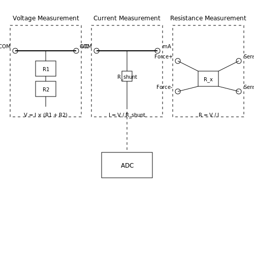
DC voltage measurements use a precision voltage divider network followed by an analog-to-digital converter (ADC). The input impedance is typically 10MΩ, though specialized meters may offer 1GΩ or higher for minimal circuit loading. AC voltage measurements first pass through a precision rectifier and RMS converter.
Current Measurement
Current measurements utilize shunt resistors of precisely known value. The voltage drop across the shunt is measured and converted to current using Ohm's Law:
High-current ranges use lower resistance shunts (often mΩ range) to minimize power dissipation and heating effects.
Resistance Measurement
Resistance measurements employ a constant current source and voltage measurement:
Four-wire Kelvin measurements eliminate lead resistance errors by using separate force and sense connections.
Advanced Features
Modern multimeters incorporate several sophisticated features:
- True RMS conversion: Essential for accurate AC measurements of non-sinusoidal waveforms
- Relative mode: Allows nulling out test lead resistance or baseline measurements
- Data logging: Records measurements over time with timestamping
- Bluetooth/USB connectivity: Enables remote monitoring and data export
- Diode test and continuity: Specialized modes with adjustable thresholds
Safety Considerations
High-end multimeters implement multiple protection mechanisms:
- High-energy varistors and spark gaps for voltage transients
- Current-limiting fuses with fast blow characteristics
- Isolation barriers for CAT III/CAT IV rated instruments
- Overload protection on all ranges
The safety category (CAT I-IV) indicates the maximum transient overvoltage the meter can withstand in different electrical environments.
2. Setting Up the Multimeter
2.1 Setting Up the Multimeter
Initial Power and Probe Configuration
Before taking measurements, ensure the multimeter is properly powered and the probes are correctly connected. Most advanced multimeters operate on a 9V battery or rechargeable cell, though bench-top models may use AC power. Insert the black probe into the COM (common) terminal and the red probe into the appropriate input jack based on the measurement type:
- Voltage, Resistance, Continuity: Red probe in the VΩ terminal.
- Current (below 10A): Red probe in the mA or A terminal.
- High Current (above 10A): Red probe in the dedicated 10A terminal.
Selecting the Measurement Mode
Rotate the dial to the desired measurement function (e.g., AC/DC voltage, current, resistance). For autoranging multimeters, the device automatically selects the optimal range. For manual ranging, start at the highest range and decrease incrementally to avoid overloading the input circuitry. Advanced models may include:
- True RMS for non-sinusoidal waveforms.
- Relative mode (Δ) for differential measurements.
- Logging mode for capturing time-series data.
Input Protection and Safety Considerations
Multimeters incorporate input protection circuits, such as PTC thermistors and spark gaps, to safeguard against transient voltages. However, exceeding the rated input limits can damage the device. For high-energy circuits, use a high-voltage probe or current clamp to isolate the multimeter. The input impedance (typically 10MΩ for voltage measurements) must be considered to avoid circuit loading effects.
Calibration and Zeroing
For precision measurements, perform an offset nulling procedure. In resistance mode, short the probes and press the REL button to subtract lead resistance. For current measurements, use the zero-adjust knob (if available) to cancel any DC offset. Calibration against a known reference (e.g., a 6½-digit calibrator) ensures traceability to NIST standards.
Advanced Features and Specialized Modes
High-end multimeters offer additional functionalities:
- 4-wire Kelvin sensing for low-resistance measurements, eliminating lead resistance errors.
- Diode test with a constant current source (typically 1mA).
- Capacitance and frequency measurement using an internal oscillator.
2.2 Measuring Voltage (AC/DC)
Fundamentals of Voltage Measurement
Voltage, the electric potential difference between two points, is a fundamental parameter in electrical systems. A multimeter measures voltage by comparing the potential at its input terminals relative to a reference (typically ground). For DC measurements, polarity matters; reversing the probes inverts the sign of the reading. AC measurements, however, are polarity-agnostic but require consideration of waveform characteristics (e.g., RMS vs. peak).
DC Voltage Measurement
When measuring DC voltage, the multimeter's internal circuitry converts the input voltage into a proportional current through a high-impedance voltage divider. The voltage Vin is calculated as:
where Im is the current through the meter movement and Rint is the internal resistance. Modern digital multimeters (DMMs) use analog-to-digital converters (ADCs) with precision reference voltages, achieving accuracies up to 0.001% in laboratory-grade instruments.
AC Voltage Measurement and RMS Conversion
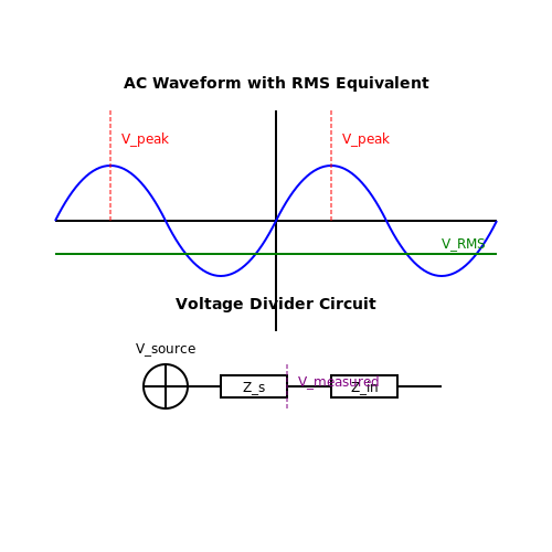
AC voltage measurement requires RMS (Root Mean Square) conversion to represent the equivalent DC power dissipation. For a sinusoidal waveform:
True RMS multimeters use thermal or computational methods to accurately measure non-sinusoidal waveforms. The error introduced by assuming a pure sine wave can be quantified using the crest factor CF:
High crest factors (common in pulsed or distorted waveforms) degrade measurement accuracy in average-responding meters.
Input Impedance and Loading Effects
The multimeter's input impedance (Zin) forms a voltage divider with the source impedance (Zs), introducing error:
High-impedance circuits (e.g., vacuum tube amplifiers) require DMMs with Zin > 10 MΩ to minimize loading. For frequencies above 1 kHz, capacitive reactance becomes significant, demanding impedance compensation in precision measurements.
Practical Considerations
- Range selection: Auto-ranging simplifies operation, but manual ranging avoids range-switching delays in dynamic measurements.
- Ground loops: Floating measurements (differential probes) prevent errors from ground potential differences.
- Bandwidth limitations: Standard DMMs attenuate signals above 500 kHz; RF measurements require specialized probes.
Advanced Techniques
For nanovolt-level measurements, integrating DMMs (e.g., Keithley 2182A) employ synchronous detection to reject noise. High-voltage measurements (>1 kV) necessitate verified CAT-rated probes and safety protocols. Oscilloscopes complement multimeters for time-domain analysis of AC signals, particularly when phase information is critical.
2.3 Measuring Current (AC/DC)
Fundamentals of Current Measurement
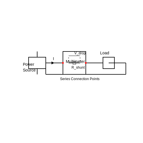
Current measurement in a multimeter relies on the principle of Ohm's Law, where the voltage drop across a known shunt resistance is used to infer the current. For DC measurements, the multimeter's internal shunt resistor (Rshunt) converts the current (I) into a measurable voltage (V):
For AC measurements, the multimeter employs a true RMS converter to accurately compute the root-mean-square value of the alternating current, accounting for non-sinusoidal waveforms. The RMS current (IRMS) is derived as:
Measurement Techniques
To measure current:
- Series Connection: The multimeter must be placed in series with the circuit, breaking the current path to allow all charge carriers to pass through the instrument.
- Range Selection: High currents (>10A) often require a separate input jack with a lower shunt resistance to minimize power dissipation and heating.
- Burden Voltage: The voltage drop across the shunt (I × Rshunt) introduces a small error, which must be considered in precision measurements.
AC Current Measurement Challenges
Unlike DC, AC measurements must account for:
- Frequency Response: Multimeters have bandwidth limitations (typically 50Hz–1kHz for standard models, up to 100kHz for precision instruments).
- Waveform Distortion: Non-linear loads (e.g., switched-mode power supplies) introduce harmonics, necessitating true RMS capability for accuracy.
- Phase Shift Errors: Inductive/capacitive loads alter the current waveform's phase relative to voltage, affecting power calculations.
Advanced Applications
In high-frequency or high-current scenarios (e.g., power electronics research), specialized methods are employed:
- Current Probes: Rogowski coils or Hall-effect sensors provide non-intrusive measurement without circuit interruption.
- Precision Shunts: Four-terminal resistors (Kelvin connections) minimize contact resistance errors.
- Oscilloscope Integration: Current probes paired with oscilloscopes capture transient behavior beyond a multimeter's bandwidth.
Safety Considerations
Current measurement poses unique hazards:
- Overload Protection: Fast-acting fuses or electronic clamping circuits prevent damage from accidental overloads.
- High-Energy Circuits: Arc flash risks necessitate fused test leads and CAT-rated equipment for industrial applications.
- Ground Referencing: Floating measurements (e.g., in switched-mode converters) require isolation to avoid ground loops.
Mathematical Derivation: Shunt Resistor Power Dissipation
The power dissipated in the shunt resistor (Pshunt) must be constrained to avoid thermal drift. For a 10A measurement with a 0.01Ω shunt:
This dissipation necessitates heat-resistant materials and derating for continuous operation.
2.4 Measuring Resistance
Fundamentals of Resistance Measurement
Resistance measurement in a multimeter is based on Ohm's Law, which states that the current I through a conductor between two points is directly proportional to the voltage V across the two points and inversely proportional to the resistance R:
Modern digital multimeters (DMMs) measure resistance by sourcing a known current through the test leads and measuring the resulting voltage drop across the component. The resistance is then calculated internally using the above relationship.
Two-Wire vs. Four-Wire Measurement
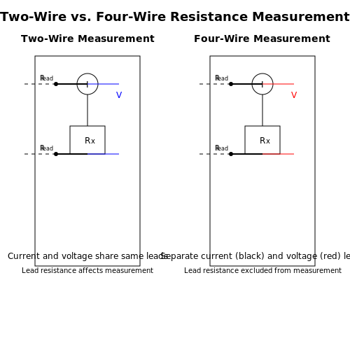
For standard measurements, two-wire resistance measurement is sufficient. However, for low-resistance values (typically below 1 Ω), lead resistance introduces significant error. In such cases, a four-wire (Kelvin) measurement is employed:
- Two-Wire Method: Current is sourced and voltage measured through the same leads. Lead resistance adds to the measured value.
- Four-Wire Method: Separate force and sense leads eliminate lead resistance errors by measuring voltage directly across the component.
Measurement Range and Resolution
Multimeters typically offer resistance ranges from milliohms (mΩ) to gigaohms (GΩ). The resolution depends on the selected range:
where N is the number of display digits. For example, a 6½-digit meter on the 1 kΩ range has a resolution of 100 μΩ.
Practical Considerations
When measuring resistance:
- Ensure the component is not powered to prevent damage to the meter.
- For high-resistance measurements (>1 MΩ), account for surface leakage currents which can affect readings.
- Use guard terminals when measuring very high resistances (>100 MΩ) to minimize stray currents.
Thermal Effects and Temperature Compensation
Resistance varies with temperature according to:
where α is the temperature coefficient of resistance. For precise measurements, either:
- Measure at known temperature and apply correction
- Use instruments with built-in temperature compensation
Advanced Techniques: AC Resistance Measurement
For components where impedance varies with frequency (e.g., inductors, capacitors), an LCR meter is more appropriate. However, some advanced DMMs can measure AC resistance by:
- Applying a small AC test signal
- Measuring both magnitude and phase of the response
- Calculating complex impedance
The impedance Z is given by:
where θ is the phase difference between voltage and current.
2.5 Continuity Testing
Continuity testing is a fundamental diagnostic technique used to verify the integrity of electrical connections, ensuring an unbroken path for current flow. Unlike resistance measurement, which quantifies opposition to current, continuity testing provides a binary indication—either a complete circuit (low resistance) or an open circuit (infinite resistance). Advanced multimeters implement this function by applying a small test voltage and measuring the resulting current, triggering an audible or visual alert if resistance falls below a predefined threshold (typically 10–50 Ω).
Principles of Operation
When a multimeter is set to continuity mode, it functions as a closed-loop system:
- A constant current source (typically 1–10 mA) is applied across the probes.
- The voltage drop Vdrop is measured and used to calculate resistance R via Ohm's Law:
If R is below the threshold, the multimeter completes an internal feedback loop, activating the alert. The response time depends on the sampling rate and filtering algorithms, with high-end instruments achieving sub-millisecond detection.
Practical Considerations for Advanced Users
While conceptually simple, continuity testing introduces several non-ideal factors that engineers must account for:
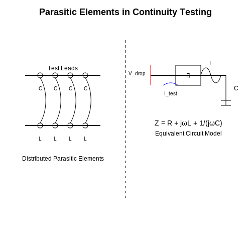
Parasitic Capacitance and Inductance
Long test leads or PCB traces introduce distributed reactance, which can distort measurements. The effective impedance Z becomes frequency-dependent:
where L and C represent parasitic inductance and capacitance, respectively. For accurate DC continuity testing, ensure the test duration exceeds the circuit's RC or L/R time constants.
Noise Immunity
In electrically noisy environments, spurious signals may trigger false positives. Modern multimeters employ:
- Digital filtering (e.g., moving average or median filters)
- Hysteresis thresholds to prevent chatter
- Guarded inputs to reduce capacitive coupling
Advanced Applications
Beyond basic wiring checks, continuity testing enables sophisticated diagnostics:
PCB Trace Verification
High-density circuit boards require continuity testing between vias and components. Automated test equipment (ATE) uses flying probes with 4-wire Kelvin sensing to eliminate lead resistance errors:
Semiconductor Junction Testing
Diode and transistor junctions exhibit nonlinear continuity characteristics. A forward-biased silicon junction typically shows 0.5–0.7 V drop, while a reverse-biased junction appears open. Specialized meters provide separate diode test modes with higher drive currents.
Instrument-Specific Implementations
Bench multimeters (e.g., Keysight 34465A) offer programmable continuity thresholds and logging capabilities. For example, setting a 5 Ω threshold with 1 ms sampling enables rapid fault detection in production testing. Handheld meters often sacrifice precision for portability, with fixed thresholds around 30 Ω.
2.6 Diode Testing
Fundamentals of Diode Testing
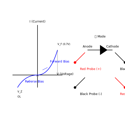
Diode testing with a multimeter relies on the principle of forward and reverse bias characteristics of a semiconductor junction. When a diode is forward-biased, it conducts current with a small voltage drop (typically 0.3 V for germanium, 0.7 V for silicon). In reverse bias, an ideal diode exhibits near-infinite resistance, though real diodes have a finite leakage current.
where I is the diode current, I0 is the reverse saturation current, VD is the applied voltage, n is the ideality factor (1 for ideal diodes), and VT is the thermal voltage (~25.85 mV at 300 K).
Multimeter Diode Test Mode
Modern digital multimeters (DMMs) include a dedicated diode test mode, which applies a small forward current (typically 1–2 mA) and measures the voltage drop. This avoids the nonlinearity of resistance-based measurements.
- Forward Bias Test: The meter displays the forward voltage drop (VF). A healthy silicon diode reads ~0.5–0.8 V.
- Reverse Bias Test: The meter should indicate an open circuit (OL or "overload"). A measurable voltage suggests leakage or breakdown.
Practical Testing Methodology
To test a diode:
- Set the multimeter to diode mode (symbol: ⎓ or →|).
- Connect the red probe to the anode and black to the cathode for forward bias.
- Reverse the probes for reverse bias verification.
Advanced Considerations
For Zener diodes, the breakdown voltage (VZ) can be measured by applying a reverse bias with a current-limiting resistor. Schottky diodes exhibit lower forward voltages (~0.2–0.4 V), while LEDs show higher drops (1.8–3.3 V) depending on material.
Dynamic Resistance
The incremental resistance (rd) of a diode is derived from the slope of the I-V curve:
where ID is the DC bias current. This parameter is critical for high-frequency and switching applications.
Real-World Applications
Diode testing is essential for:
- Fault Detection: Identifying shorted or open diodes in rectifiers.
- Quality Control: Verifying VF consistency in production batches.
- Circuit Debugging: Isolating failed components in power supplies and signal paths.
3. Handling High Voltage and Current
3.1 Handling High Voltage and Current
When measuring high voltage or current with a multimeter, safety and precision are paramount. Exceeding the rated input limits of the instrument can result in catastrophic failure, including arcing, component damage, or personal injury. Multimeters typically specify maximum voltage (e.g., 1000V CAT III) and current (e.g., 10A) ratings, which must never be surpassed without proper external attenuation.
Voltage Measurement Considerations
High-voltage measurements require specialized probes with sufficient insulation and voltage derating. The input impedance of a multimeter (typically 10MΩ for DC) forms a voltage divider with the source impedance, introducing measurement errors if not accounted for. For AC measurements, the frequency response of the probe and meter must be considered, as capacitive coupling can distort readings at high frequencies.
For voltages above 1kV, external high-voltage probes with known attenuation ratios (e.g., 1000:1) should be used. These probes incorporate high-value series resistors (often 100MΩ to 1GΩ) to limit current while maintaining accuracy.
Current Measurement Techniques
Direct current measurement through a multimeter's internal shunt resistor is limited by power dissipation:
For currents exceeding 10A, clamp-on current probes or external shunts with proper voltage isolation are required. Hall-effect sensors are preferable for AC measurements, while Rogowski coils provide bandwidth advantages for pulsed currents.
Safety Protocols
- Always verify meter category rating (CAT I-IV) matches the measurement environment
- Use proper personal protective equipment (PPE) including insulated gloves when working above 50V
- Employ the "one-hand rule" when probing live circuits to prevent current pathways through the body
- Verify meter functionality on a known source before and after high-energy measurements
Transient Protection
High-energy transients require additional protection components. Multimeters designed for power systems incorporate:
- Metal oxide varistors (MOVs) for voltage clamping
- Gas discharge tubes for high-current diversion
- Fast-acting fuses with current-limiting designs
The time-energy integral of protective devices must exceed anticipated fault conditions:
Practical Implementation
When measuring three-phase systems, ensure proper phase synchronization and use differential probes for floating measurements. For pulsed power applications, consider the meter's crest factor rating and sampling rate to capture true peak values. Always de-energize systems before changing measurement modes to prevent shunt resistor damage during voltage measurements.
3.2 Avoiding Common Mistakes
Even experienced engineers and researchers can make critical errors when using multimeters, leading to inaccurate measurements, equipment damage, or safety hazards. Understanding these pitfalls and adopting best practices ensures reliable results and prolongs instrument lifespan.
Incorrect Range Selection
Auto-ranging multimeters mitigate this issue, but manual range selection remains common in precision measurements. Selecting a range too low for the measured quantity can overload the instrument, while an excessively high range reduces resolution. For voltage measurements, always start at the highest range and step down. Current measurements require careful consideration of the expected load:
where Imax determines the appropriate current range. Exceeding the multimeter's current rating, typically 10A for most models, risks blowing the internal fuse or damaging shunt resistors.
Improper Lead Configuration
A frequent error involves leaving leads in the current measurement jacks when measuring voltage, which creates a near-short circuit if connected across a voltage source. The correct configuration follows:
- Voltage/Resistance/Diode Test: COM (black) and VΩ (red) jacks
- Current Measurement: COM (black) and A/mA (red) jacks
- High Current (>200mA): Use dedicated 10A jack if available
Ignoring Input Impedance Effects
Digital multimeters typically have 10MΩ input impedance on voltage ranges. While negligible for low-impedance circuits, this becomes significant when measuring high-resistance voltage dividers or sensitive analog circuits. The loading error can be calculated as:
For example, measuring a 1MΩ source with a 10MΩ meter introduces a 9.1% error. In such cases, use a meter with higher input impedance (1GΩ or more) or employ null measurement techniques.
AC vs DC Coupling Confusion
When measuring AC signals superimposed on DC offsets, improper coupling leads to erroneous readings. True-RMS meters measure the combined AC+DC value in AC mode unless explicitly using AC-coupled ranges. The correct calculation for power in such scenarios is:
This becomes particularly critical when measuring ripple in power supplies or audio signal analysis.
Thermal EMF Errors
In low-voltage resistance measurements (especially below 1Ω), thermoelectric voltages from dissimilar metal junctions introduce significant errors. The Seebeck coefficient for common lead materials ranges from 1-50 μV/°C. To minimize this effect:
- Use copper test leads with gold-plated connectors
- Employ the offset compensation function (REL or zero) after lead connection
- Maintain stable ambient temperature during measurement
Ground Loop Artifacts
When measuring voltages in grounded systems, improper multimeter connection can create ground loops that distort measurements. The voltage error introduced by ground current Ig flowing through lead resistance Rlead is:
This manifests as unstable readings or unexpected offsets. Solutions include using differential voltage measurements, battery-powered meters, or isolation amplifiers for floating measurements.
Probe Compensation in Capacitance Measurements
High-frequency capacitance measurements require probe compensation to account for parasitic elements. The total measured capacitance Cmeas includes:
where Cstray represents stray capacitance (typically 50-100pF) and Llead is lead inductance. Use guarded measurements and null the probe capacitance before testing critical components.
3.3 Proper Maintenance and Calibration
Calibration Standards and Traceability
Multimeter calibration must adhere to internationally recognized standards such as ISO/IEC 17025 or ANSI/NCSL Z540-1. Traceability to primary standards maintained by national metrology institutes (e.g., NIST, PTB) is essential for ensuring measurement accuracy. The calibration process typically involves comparing the multimeter's readings against a reference standard with at least four times higher precision (4:1 TUR - Test Uncertainty Ratio).
Where δ represents the percentage error, which should remain within the manufacturer's specified tolerance band across all measurement ranges.
Environmental Control
Calibration environments must maintain:
- Temperature stability within ±1°C of 23°C (per IEC 60751)
- Relative humidity between 45% and 55%
- Electromagnetic interference below 1 V/m from 10 kHz to 1 GHz
- Vibration isolation with RMS displacement < 0.1 µm
Preventive Maintenance Procedures
A comprehensive maintenance schedule should include:
Contact Maintenance
Test lead contacts degrade through oxidation and mechanical wear. Clean gold-plated contacts monthly with isopropyl alcohol (99.9% purity) and inspect for pitting using 10× magnification. Nickel-plated contacts require more frequent cleaning (weekly) with contact enhancer solutions.
Internal Component Inspection
For analog multimeters, check for:
- Magnet strength degradation (should maintain > 95% of initial flux density)
- Pivot bearing wear (axial play < 5 µm)
- Coil resistance drift (< ±0.5% from nominal)
Digital multimeters require verification of:
- Reference voltage stability (e.g., LTZ1000 drift < 2 ppm/√kHr)
- Input protection components (MOVs, PTCs) for degradation
- ADC linearity error (< 1 LSB)
Calibration Interval Determination
The optimal calibration interval can be calculated using the historical stability method:
Where I represents the interval in months, and U is the observed versus allowable uncertainty ratio. For critical applications, Bayesian statistical models may be employed to predict out-of-tolerance probabilities.
Field Calibration Techniques
When laboratory calibration isn't feasible, field calibration using portable metrology-grade references (e.g., Fluke 5522A) can maintain accuracy. Key considerations include:
- Warm-up time compensation (typically 4× manufacturer specification)
- Thermal EMF correction for low-voltage measurements
- Guard banding of ±0.2% for critical measurements
Automated Calibration Systems
Modern calibration systems utilize:
- IEEE 488.2 command sets for instrument control
- Monte Carlo simulations for uncertainty analysis
- Blockchain-based calibration records for audit trails
Advanced systems implement machine learning algorithms that analyze historical calibration data to predict component drift patterns and optimize maintenance schedules.
4. Capacitance Measurement
4.1 Capacitance Measurement
Fundamentals of Capacitance Measurement
Capacitance, defined as the ability of a system to store charge per unit voltage, is measured in farads (F). A multimeter measures capacitance by applying a known AC or DC excitation and analyzing the resultant current and phase shift. The fundamental relationship governing capacitance is:
where C is capacitance, Q is charge, and V is voltage. Advanced multimeters employ impedance spectroscopy or time-domain analysis to derive capacitance accurately.
Measurement Techniques
Modern digital multimeters (DMMs) use one of two primary methods:
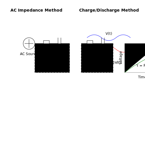
- AC Impedance Method: Applies a sinusoidal signal and measures the reactance (XC). The capacitance is derived from:
where f is the excitation frequency.
- Charge/Discharge Method: Measures the time constant (τ = RC) of a known resistor-capacitor network. The capacitance is calculated via:
Practical Considerations
Accurate capacitance measurement requires compensating for:
- Parasitic Effects: Stray inductance and resistance alter readings, particularly at high frequencies.
- Dielectric Absorption: Residual charge in dielectrics can skew results, necessitating discharge cycles before measurement.
- Frequency Dependence: Electrolytic and ceramic capacitors exhibit varying capacitance with frequency, requiring matched test conditions.
Advanced Applications
Precision capacitance measurements are critical in:
- Semiconductor Characterization: Determining gate oxide capacitance in MOSFETs.
- Material Science: Measuring permittivity of novel dielectrics.
- RF Circuit Design: Tuning matching networks via accurate capacitor selection.
Error Sources and Mitigation
Common errors include:
- Lead Resistance: Minimized using Kelvin connections.
- Ground Loops: Eliminated via shielded probes and differential measurements.
- Temperature Drift: Compensated using temperature-stable references.
4.2 Frequency Measurement
Fundamentals of Frequency Measurement
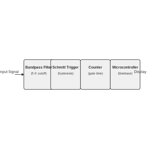
Frequency, defined as the number of cycles per second (Hz), is a critical parameter in AC signal analysis, RF applications, and digital systems. Modern multimeters measure frequency by counting zero-crossings or threshold crossings of the input signal over a precisely timed interval. The internal timebase of the multimeter, typically derived from a crystal oscillator with stability in the ppm range, ensures accuracy.
where N is the number of cycles counted and T is the measurement window. For signals with harmonic distortion or noise, advanced multimeters employ Schmitt triggers or digital filtering to reject false triggers.
Measurement Techniques and Limitations
Direct counting is the most common method for frequencies below 100 kHz, while reciprocal counting (measuring the period and inverting it) improves accuracy for lower frequencies. High-frequency measurements (>1 MHz) often require prescalers or heterodyne techniques due to limitations in the multimeter’s internal clock speed.
Key Error Sources
- Trigger jitter: Noise or slew rate limitations cause timing uncertainty.
- Timebase drift: Crystal oscillator instability over temperature.
- Aliasing: Undersampled signals create false frequency readings.
Advanced Applications
In power electronics, frequency measurement verifies PWM signals and inverter outputs. For RF work, multimeters with bandwidths up to 10 GHz (via external downconverters) characterize carrier waves. Digital protocols like I²C or SPI may require duty cycle analysis alongside frequency.
Calibration and Traceability
High-precision frequency measurements require traceable calibration against atomic standards (e.g., Rb or Cs clocks). The Allan variance metric characterizes short-term stability, while linearity tests verify the multimeter’s response across its full range.
where σy(τ) is the Allan deviation for averaging time τ, and yi represents fractional frequency measurements.
4.3 Temperature Measurement
Thermocouple Principles and Seebeck Effect
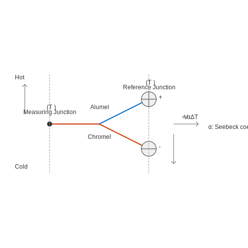
Temperature measurement using multimeters primarily relies on thermocouples, which operate based on the Seebeck effect. When two dissimilar metals are joined at one end (the measuring junction) and subjected to a temperature gradient, a voltage proportional to the temperature difference is generated across the free ends (the reference junction). The relationship is given by:
where V is the thermoelectric voltage, α is the Seebeck coefficient (µV/°C), and Tmeas and Tref are the temperatures at the measuring and reference junctions, respectively. For type-K thermocouples (chromel-alumel), α ≈ 41 µV/°C.
Cold Junction Compensation (CJC)
Since the output voltage depends on the temperature difference between junctions, multimeters must compensate for the reference junction temperature (Tref). Modern instruments use an integrated thermistor or RTD to measure Tref and adjust the output accordingly. The corrected temperature is computed as:
Practical Implementation in Multimeters
Advanced multimeters with temperature measurement capabilities typically include:
- Type-K thermocouple inputs with mini-connectors (e.g., Fluke 87V).
- Automatic CJC via an internal sensor near the input terminals.
- Linearization algorithms to convert the nonlinear Seebeck voltage to temperature (e.g., NIST ITS-90 polynomials).
Error Sources and Mitigation
Key error contributors include:
- Thermal gradients at the reference junction (minimized by shielding and isothermal blocks).
- Thermocouple aging due to oxidation (addressed by using sheathed probes).
- Electrical noise (reduced via twisted-pair wiring and differential measurement).
Alternative Methods: RTDs and Thermistors
Some multimeters support resistive temperature detectors (RTDs) or thermistors by measuring resistance and applying the Steinhart-Hart equation:
where A, B, and C are device-specific coefficients. Platinum RTDs (PT100) offer ±0.1°C accuracy but require 4-wire measurement to eliminate lead resistance errors.
Calibration and Traceability
For laboratory-grade applications, multimeter temperature functions must be calibrated against NIST-traceable standards using:
- Dry-block calibrators (±0.02°C stability).
- Ice-point cells (0.0°C reference).
- Thermocouple simulators for voltage-to-temperature verification.
4.4 Data Logging and Connectivity Features
Data Logging Capabilities
Modern high-end multimeters incorporate data logging functionalities, enabling the recording of measurements over time for post-processing and analysis. The sampling rate, storage capacity, and resolution are critical parameters determining the effectiveness of data logging. For instance, a multimeter with a 16-bit analog-to-digital converter (ADC) and a sampling rate of 1 kHz can capture transient events with microsecond-level precision. The logged data is typically stored in non-volatile memory, with formats such as CSV or binary for efficient retrieval.
where N is the total number of samples, fs is the sampling rate, and T is the logging duration. Higher sampling rates demand greater storage capacity, often necessitating external memory solutions for long-duration captures.
Connectivity Interfaces
Advanced multimeters support multiple connectivity options to interface with computers, networks, or other instruments:
- USB – Provides plug-and-play compatibility with PCs for real-time data streaming and remote control via SCPI (Standard Commands for Programmable Instruments) commands.
- Bluetooth/Wi-Fi – Enables wireless data transfer to mobile devices or cloud platforms, facilitating remote monitoring in industrial environments.
- GPIB/IEEE-488 – A legacy but robust interface for automated test systems, offering high-speed communication in laboratory settings.
- Ethernet (LAN) – Supports network-based integration, allowing multimeters to be part of distributed measurement systems with centralized data logging.
Real-World Applications
In power quality analysis, multimeters with high-speed logging capabilities capture voltage sags, swells, and harmonic distortions. For battery testing, continuous current and voltage logging helps assess charge-discharge cycles. Industrial automation leverages networked multimeters for predictive maintenance by monitoring motor currents and detecting anomalies before failure.
Software Integration
Manufacturers provide proprietary software (e.g., Keysight BenchVue, Fluke Connect) for configuring multimeters, visualizing data, and exporting results. Open-source alternatives like PyVISA enable Python-based automation, allowing custom scripts to control multimeters programmatically. For example:
import pyvisa
rm = pyvisa.ResourceManager()
multimeter = rm.open_resource("USB0::0x2A8D::0x0101::MY12345678::INSTR")
voltage = multimeter.query("MEAS:VOLT:DC? 10,0.001")
Synchronization in Multi-Channel Systems
Precision timing protocols such as IEEE 1588 (PTP) synchronize multiple multimeters in distributed systems, ensuring coherent sampling across channels. This is crucial in phased-array measurements or power grid monitoring, where sub-millisecond alignment is required.
5. Diagnosing Faulty Readings
5.1 Diagnosing Faulty Readings
When a multimeter produces unexpected or inconsistent measurements, systematic troubleshooting is required to isolate the source of error. Faulty readings typically stem from one of four categories: instrument limitations, improper configuration, measurement technique errors, or circuit loading effects.
Instrument Limitations and Calibration
All multimeters have inherent accuracy limits specified by their manufacturer. A 3½-digit meter with ±1% accuracy on the 20 V DC range has a potential error of:
Calibration drift occurs over time due to component aging. To verify, measure a known voltage reference source like a LM4040 precision shunt regulator. If readings fall outside the multimeter's specified tolerance, recalibration is necessary using traceable standards.
Configuration Errors
Common setup mistakes include:
- AC mode selected for DC measurements (or vice versa)
- Incorrect range selection causing overflow or loss of significant digits
- Enabled relative mode (Δ) without proper zeroing
- Active low-pass filtering distorting high-frequency signals
For resistance measurements, ensure the circuit is powered off and capacitors are discharged. A diode check function may give false readings if testing parallel resistive paths.
Measurement Technique Artifacts
High-impedance circuits are particularly susceptible to loading errors. A 10 MΩ input impedance multimeter measuring a 1 MΩ voltage divider introduces a 9.1% error:
Thermal EMFs in test leads can generate microvolt-level offsets in low-voltage measurements. Use gold-plated contacts and copper leads to minimize this effect.
Circuit Loading and Bandwidth Effects
When measuring AC signals, consider the multimeter's bandwidth limitations. A typical handheld DMM has a 3 dB bandwidth of 1-5 kHz for AC voltage measurements. The measured RMS value of a 10 kHz square wave may appear attenuated due to the limited frequency response.
Current measurements introduce series resistance through the shunt. A 10 A range with 0.01 Ω shunt drops 100 mV per amp, potentially affecting low-voltage circuits. Use the highest possible range that maintains sufficient resolution to minimize voltage burden.
For high-frequency measurements, probe capacitance becomes significant. A 100 pF input capacitance forms a low-pass filter with circuit impedance:
5.2 Identifying and Fixing Connection Problems
Diagnosing Poor Electrical Contacts
Intermittent or high-resistance connections are a common source of measurement error in multimeter circuits. The contact resistance Rc between probes and test points follows:
where ρ is the resistivity of the contact material, a is the radius of actual contact spots (typically microscopic due to surface roughness), and d is the apparent contact diameter. For oxidized copper probes at 1N force, Rc can exceed 10Ω.
Four-Wire Kelvin Measurement
When contact resistance dominates the measurement, employ four-terminal sensing:
The current excitation (I+, I-) and voltage sensing (V+, V-) paths are separated, eliminating voltage drops across probe contacts from the measurement.
Probe Selection Criteria
Optimize probe choice based on:
- Tip geometry: Sharp needles (≤0.5mm) for PCB pads, flat blades for terminals
- Contact force: ≥3N for gold-plated, ≥5N for nickel surfaces
- Shielding: Guarded probes reduce capacitive coupling in high-impedance circuits
Troubleshooting Sequence
- Verify continuity between probe tips (should read <0.5Ω with shorted inputs)
- Check for thermoelectric voltages by reversing probe polarity
- Measure contact resistance variation under mechanical wiggling
- Inspect for fretting corrosion using 10× magnification
High-Frequency Considerations
Above 1MHz, probe inductance Lp dominates:
where Cp is the stray capacitance (typically 10-50pF). Use coaxial probes with ground rings for RF measurements.
5.3 When to Replace Your Multimeter
Accuracy Drift Beyond Acceptable Tolerance
Multimeters experience gradual accuracy degradation due to component aging, thermal stress, and mechanical wear. For high-precision applications, verify calibration against a known reference source. If measurements consistently deviate beyond the manufacturer's specified tolerance (typically ±0.5% to ±2% for advanced models), recalibration may not suffice. The uncertainty contribution Umeter to a measurement system should satisfy:
where Usystem is the total permissible uncertainty budget. When this condition fails despite recalibration, replacement becomes necessary.
Physical Damage Affecting Measurement Integrity
Inspect for:
- Cracked or distorted input jacks causing intermittent connections
- Damaged rotary switch contacts producing erratic range selection
- Compromised case integrity exposing internal circuits to contaminants
High-voltage incidents may carbonize PCB traces without visible damage. Perform a dielectric strength test (500V–1000V DC) between isolated channels if the multimeter has survived electrical overstress.
Obsolete Technology Limitations
Legacy multimeters may lack critical modern features:
- True RMS capability for non-sinusoidal waveforms
- Bluetooth/logging interfaces for automated data collection
- Category III/IV safety ratings for modern power systems
The update rate of older models (often below 3 samples/second) becomes inadequate for capturing transient phenomena in power electronics or motor drive analysis.
Battery Drain and Power System Failure
Excessive battery consumption (e.g., draining a fresh 9V battery in under 30 days) indicates leakage currents in the power management circuit. For bench multimeters, failing power supplies manifest as:
- Display flickering during autoranging
- Inconsistent backlight intensity
- Spontaneous resets during measurement
These symptoms often precede complete power subsystem failure.
Display Degradation and Interface Issues
Persistent segments in LCDs or unresponsive touch interfaces compromise usability. For OLED displays, uneven pixel aging creates visibility challenges in low-light lab environments. When display-related errors exceed 5% of reading time during critical measurements, consider replacement.
Software/Firmware Obsolescence
Multimeters with discontinued firmware support cannot address:
- New communication protocols (SCPI 2020+ revisions)
- Security vulnerabilities in networked operation
- Compatibility with modern calibration standards (ISO/IEC 17025:2017)
Manufacturers typically provide 7–10 years of firmware updates for professional-grade instruments.
Cost-Benefit Analysis of Repair vs Replacement
Evaluate using:
where Crepair is repair cost, Mannual is projected annual maintenance, and Cnew is current market price. The 0.6 coefficient accounts for improved features in newer models.
6. Recommended Books and Manuals
6.1 Recommended Books and Manuals
- Keithley Low Level Measurements Handbook - 7th Edition — 1.1 In troduction. DC voltage, DC current, and resistance are measured most often with digital multimeters (DMMs).Generally, these instruments are adequate for measurements at signal levels greater than 1µV or 1µA, or less than 1G W. (See Figure 1-1 for standard symbols used in this text.) However, they don't approach the theoretical limits of sensitivity.
- PDF Physics 115 Electronics and Instrumentation Laboratory Manual — This manual will also likely serve as a reference for future classwork, particularly in Physics 116, Advanced Electronics and Instrumentation. I suggest that if you are planning on taking this course, you hold onto this book. This is the sixth edition of this manual; it is mainly for correcting some errors and restructuring some experiments.
- Electronic Measurements and Instrumentation[Book] - O'Reilly Media — Electronic Measurements and Instrumentation provides a comprehensive blend of the theoretical and practical aspects of electronic measurements and instrumentation. It provides a comprehensive coverage of each topic in the syllabus … - Selection from Electronic Measurements and Instrumentation [Book]
- Digital multimeter - Free Pdf Manuals Download | ManualsLib — View and download Digital multimeter manuals for free. Digital Multimeter CP7676 instructions manual. Sign In Upload. Filter results: Brands . UNI-T 38; Kusam-meco 26; Amprobe 25; Velleman 25; Fluke 24; Agilent Technologies ...
- K. Lal Kishore - Electronic Measurements & Instrumentation-Pearson ... — Hence, in electronic multimeters, the resistance values increase from left to right similar to 60 Electronic Measurements and Instrumentation Figure 1.68 Typical input voltage attenuator for a VOM. The range switch on the front of the panel of the VOM allows selection of the desired voltage range
- PDF ECE 311 LABORATORY MANUAL - Clemson University — Nigro who retyped the complete revised manual. K F Poole Jan 2004 Version 1.2 The manual has undergone a comprehensive review over the past year. Thanks to David Epting who has tracked and corrected the errors in version 1.1 and suggested many improvements throughout the manual. Thanks to Janet Bean for preparing the 2005 version 1.2 laboratory ...
- PDF SYLLABUS PART A UNIT 1 - WordPress.com — An electronic instrument is the one which is based on electronic or electrical principles for its measurement function. The measurement of any electronic or electrical quantity or variable is termed as an electronic measurement. Advantages of Electronic Measurement The advantages of an electronic measurement are 1.
- PDF ELECTRICAL MEASUREMENTS & INSTRUMENTATION - Veer Surendra Sai ... — assignments by referring the text books and reference books. Further, this document is not ... Accuracy of measurement, Electronic Voltmeter: Transistor Voltmeter, Block diagram, principle of operation, various types of electronic voltmeter, Digital Frequency meter: Block diagram, principle of operation TEXT BOOKS [1]. A Course in Elec ...
- PDF Industrial Electronic Circuits Laboratory Manual - Springer — manual of devices that you will use during the experiments. Another good reference is your laboratory instructor. Studying the Ref. [1] is recommended as well. 1.2 Digital Multi Meter (DMM) Digital multimeters are measuring instruments that can measure quantities such as voltage, current, and resistance.
- PDF Chapter-8 Electronic Measurements and Measuring Instruments — The whole operation of the device is based on electronic components. 6.3 Multimeter Multimeter or a multitester is a measurement instrument used in electronics, which is designed to perform tasks of several measuring instruments. The voltage, current, and resistance measurements can be made using different options available in a common Multimeter.
6.2 Online Resources and Tutorials
- PDF Solution Electronic Instruments And Measurements Larry (PDF) — A: Numerous online resources, textbooks, and courses are available. Consider searching for tutorials on YouTube or taking online courses from platforms like Coursera or edX. Remember, like Larry, embrace the challenge, be patient, and never stop learning! The world of electronic instruments and measurements is vast and rewarding. Happy measuring!
- Readings | Circuits and Electronics | Electrical Engineering and ... — Agarwal, Anant, and Jeffrey H. Lang. Foundations of Analog and Digital Electronic Circuits. San Mateo, CA: Morgan Kaufmann Publishers, Elsevier, July 2005. ISBN: 9781558607354. View e-book version. Elsevier companion site: supplementary sections and examples. Readings with an asterisk (*) provide key intuitive analyses.
- Multimeter - Introduction to electronic lab tools — Instead of m, some multimeters will include the number 2 in different magnitudes, such as: 2, 20, 200, 2000. Fun fact on why the number 2 is used (hint: it's related to 7-segment displays). The unit measured is voltage and amps respectively, with the scaling dependent on the range being measured.
- PDF Chapter-8 Electronic Measurements and Measuring Instruments — The whole operation of the device is based on electronic components. 6.3 Multimeter Multimeter or a multitester is a measurement instrument used in electronics, which is designed to perform tasks of several measuring instruments. The voltage, current, and resistance measurements can be made using different options available in a common Multimeter.
- 6.02 Tutorial 1 | Introduction to EECS II: Digital Communication ... — This resource contains information regarding tutorial 1. Browse Course Material Syllabus Software Calendar ... This resource contains information regarding tutorial 1. Resource Type: Tutorials. pdf. 168 kB 6.02 Tutorial 1 Download File Course Info Instructors Prof. Hari Balakrishnan ...
- PDF Me 360: Fundamentals of Signal Processing, Instrumentation and Control — measured with the digital multimeter. (i) Use the gain and phase shift to calculate the filter time constant . Use the time constant and the measured resistance R to find the unknown capacitance of the filter capacitor. 5. BACKGROUND In this experiment, we consider three of the most useful general-purpose electronic instruments available;
- Working Principle of Digital Multimeter: - EEEGUIDE — All Working Principle of Digital Multimeter employ some kind of analog to digital (A/D) converters (often dual slope integrating type) and have a visible readout display at the converter output. Panel meters are usually placed at one location (and perhaps even a fixed range), while bench meters and system meters are often multimeters, i.e. they ...
- PDF ELECTRICAL MEASUREMENTS & INSTRUMENTATION - Veer Surendra Sai ... — Modern Electronic Instrumentation and Measurement Techniques: Helfrick & Cooper [3]. Electrical Measurement and Measuring Instruments - Golding & Waddis . CLASS NOTES ON ELECTRICAL MEASUREMENTS & INSTRUMENTATION 2015 4 Model Question Paper: Set-1 Full Marks: 70 Time: 3 hours Answer any six ...
- How to use multimeter - Robo India || Tutorials - Learn Arduino — Robo India in this tutorial explains how to use multimeter with illustrated diagrams. 1. Multimeter: 2. Test leads ( Red and Black): 3. A complete Multimeter: 4. DC Voltage Measurement: 4.1. Connect test leads as shown in the picture. 4.2 Set rotary switch to the position as shown in the picture.
- PDF Tutorial - Building circuits & using a multimeter - University of Ottawa — The multimeter You might have already seen or worked with a multimeter. It is an electronic measuring device that combines several instruments such as the voltmeter (to measure the voltage) or the ammeter (to measure the current) in one apparatus. The multimeter is usually a standalone instrument that you can carry around to do measurements.
6.3 Industry Standards and Safety Guidelines
- IEC 61010-2-033:2023 - Safety requirements for ... - iTeh Standards — IEC 61010-2-033:2023 specifies safety requirements for hand-held multimeters and other meters for domestic and professional use, capable of measuring mains. Hand-held multimeters are multi-range multifunction measuring instruments intended to measure voltage and other electrical quantities such as resistance or current. Their primary purpose is to measure voltage on a live mains. They are ...
- IEC61010 3rd edition: New international safety requirements for lab ... — The electronic components resource for engineers and purchasers ... The IEC has published the third edition of the safety Standard for Measurement, Control and Laboratory Equipment, IEC61010-1. ... also led the development of two part 2 standards for IEC61010: IEC61010-2-033, Particular requirements for Hand-Held Multimeters and other Meters ...
- Iec 61326-1:2020 — International Standard: Publication date: 2020-10-26: Edition: 3.0: ICS: 17.220.20 ... is the world's leading organization for the preparation and publication of international standards for all electrical, electronic and related technologies. ... climate change mitigation, and increases the safety of people and the environment. Associated ...
- PDF Measuring and Testing Safely - Guide - staubli.com — applicable standards and directives, this bro-chure also addresses current changes to the industry standard IEC 61010-031, the most important standard for the safety of electro-technical test accessories. We've also included in this brochure, a glos-sary with explanations of terms related to measurement and test accessories.
- Specifications and Tolerances for Reference Standards and Field Stan — These specifications are not intended to make obsolete those field standards fabricated to meet other specifications. All new provers must meet these requirements prior to certification for legal use. 1.3 Safety Considerations This standard may involve hazardous materials, operations, and equipment. This standard does not purport to address
- PDF Specifications and Tolerances for Reference Standard and Field Standard ... — The accuracy and repeatability of field standards is critically dependent upon cleanliness. Chemicals used in the cleaning process should be evaluated for safety in use and for appropriate disposal methods by reviewing Safety Data Sheets (SDS ), formerly known as Material Safety Data Sheets (MSDS).
- PDF A Guide to United States Electrical and Electronic Equipment ... - NIST — This guide addresses electrical and electronic consumer products, including those that will . In addition, it includes electrical and electronic products used in the workplace as well as electrical and electronic medical devices. The scope does not include vehicles or components of vehicles, electric or electronic toys, or recycling ...
- PDF Multimeter safety by the numbers - Transcat — publishes international standards for all electri-cal, electronic and related technologies. Multimeters designed to the IEC ANSI 61010-1 standard offer a significantly higher level of safety. CAT 0 IEC measurement categories are based on the fact that a dangerous high-energy transient, such as a
- PDF Guidelines on the Calibration Digital Multimeters - EURAMET — 1.1 The aim of this document is to provide guidelines on the Calibration of Digital Multimeters (DMM) for accredited calibration Laboratories (ACL). In the absence of specific international written standards on DMMs, this document supplements the manufacturer's recommendations and the calibration procedures of the ACLs.
- Guide to digital multimeter safety - Fluke Corporation — At Fluke, we safety test our products, pushing them to the limit.It's only when the test team can no longer get a unit to fail that it can be released into production. The goal is to ensure a Fluke digital multimeter can repeatedly withstand the most demanding real-world conditions and keep you, the user, safe and heading home every single day.