Using a Digital Multimeter
1. What is a Digital Multimeter?
What is a Digital Multimeter?
A digital multimeter (DMM) is an electronic measuring instrument that combines multiple measurement functions into a single compact unit, typically capable of measuring voltage, current, and resistance with high precision. Unlike analog multimeters, which rely on a moving coil mechanism and a needle to display readings, DMMs utilize an analog-to-digital converter (ADC) to process input signals and display results numerically on an LCD or LED screen. This digital approach offers superior accuracy, resolution, and ease of use, making DMMs indispensable in both laboratory and field applications.
Core Components and Operation
The fundamental architecture of a DMM consists of several key subsystems:
- Input Conditioning Circuitry: Attenuates or amplifies input signals to match the dynamic range of the ADC. High-voltage measurements, for instance, employ precision resistor dividers to scale down the input.
- Analog-to-Digital Converter (ADC): The heart of the DMM, typically a dual-slope integrating converter or a successive approximation register (SAR) type, which converts analog signals into digital values. The ADC's resolution, often 3½ to 4½ digits (equivalent to 2000 to 20000 counts), directly determines the instrument's precision.
- Digital Display: Presents measured values numerically, often with additional information such as units, range, and warning indicators (e.g., overload).
- Range Selection: Manual or auto-ranging switches adjust the measurement scale to optimize resolution and prevent saturation.
The mathematical relationship between the input signal and the displayed value for DC voltage measurements can be derived as follows:
where \( N_{ADC} \) is the ADC output code, \( n \) is the ADC resolution in bits, \( V_{ref} \) is the reference voltage, and \( R_1 \), \( R_2 \) form the input divider network.
Practical Considerations and Advanced Features
Modern DMMs incorporate features that extend their utility in advanced applications:
- True RMS Conversion: Sophisticated DMMs compute the root-mean-square value of AC signals, essential for non-sinusoidal waveforms. This involves squaring the input, averaging over time, and taking the square root mathematically:
- High-Impedance Inputs: Input impedances exceeding 10 MΩ minimize circuit loading during voltage measurements.
- Guard Terminal: Used in high-resistance measurements to eliminate leakage currents by actively driving shield conductors at the same potential as the measured node.
- Four-Wire Kelvin Resistance Measurement: Eliminates lead resistance effects by using separate force and sense connections, critical for sub-ohm measurements.
The evolution of DMM technology has been driven by the need for higher precision in metrology applications. Contemporary laboratory-grade instruments achieve basic DC voltage accuracies better than 0.002%, with thermal EMF compensation, low-noise input amplifiers, and sophisticated calibration routines. The transition from discrete component designs to application-specific integrated circuits (ASICs) has enabled this performance while reducing size and power consumption.
In research environments, specialized DMM variants offer additional capabilities such as scanning multimeter functionality (multiple input channels), data logging interfaces (GPIB, USB, Ethernet), and synchronization with other instruments for automated test systems. The integration of digital signal processing allows for advanced analysis, including statistical evaluation of measurements and real-time filtering of noisy signals.

1.2 Key Components and Features
Display and Measurement Resolution
The digital display of a multimeter is characterized by its counts and digits, which determine measurement resolution. A 3½-digit display can show values up to 1999 counts, while a 4½-digit display extends to 19999 counts. High-precision benchtop multimeters may offer 6½ or 8½ digits, enabling resolution at the microvolt or nanoampere level. The effective number of bits (ENOB) in the analog-to-digital converter (ADC) directly impacts this resolution:
where SINAD is the signal-to-noise and distortion ratio. Modern multimeters often employ delta-sigma ADCs with 24-bit resolution for high-accuracy DC measurements.
Input Terminals and Guarding
Multimeters feature multiple input terminals for voltage, current, and resistance measurements. High-end models implement guarded inputs to minimize leakage currents, with the guard terminal actively driven to the same potential as the high-impedance input. This technique reduces parasitic capacitance effects when measuring resistances above 1 GΩ. The input impedance typically follows:
where \( R_{in} \) often exceeds 10 GΩ and \( C_{in} \) ranges from 100-500 pF in professional-grade instruments.
Range Switching Architecture
Auto-ranging multimeters utilize relay-based or solid-state switching networks to select appropriate measurement ranges. The switching time \( \tau_{switch} \) involves both mechanical (for relays) and settling time components:
High-speed designs employ FET switches with \( \tau_{switch} < 1 \) ms, while precision measurements may use mercury-wetted relays despite slower switching (10-50 ms) for superior contact stability.
Reference Voltage and Calibration
The voltage reference circuit determines the absolute accuracy of all measurements. Precision multimeters use oven-controlled Zener references (e.g., LTZ1000) with temperature coefficients below 0.05 ppm/°C. The reference voltage \( V_{ref} \) exhibits long-term drift modeled by:
where \( A \) represents random walk noise, \( B \) accounts for aging effects, and \( C \) captures environmental dependencies. Regular calibration against traceable standards compensates for these drifts.
Current Measurement Shunts
Current ranges employ precision shunts with temperature-compensated resistance alloys like Manganin or Zeranin. The power dissipation \( P_{shunt} \) must be carefully managed to avoid self-heating errors:
where \( \Delta T \) is the maximum allowable temperature rise and \( heta_{JA} \) is the thermal resistance. High-current ranges (10A+) often incorporate active cooling or pulsed measurement techniques.

1.3 Types of Digital Multimeters
Digital multimeters (DMMs) are classified based on their measurement capabilities, resolution, accuracy, and specialized functionalities. The primary distinctions arise from their architecture, sampling methods, and application-specific optimizations.
1.3.1 General-Purpose DMMs
These are the most common type, offering standard measurement ranges for voltage (AC/DC), current (AC/DC), resistance, continuity, and diode testing. Their resolution typically ranges from 3½ to 4½ digits (e.g., 1999 to 19999 counts), with basic accuracy of ±0.5% to ±1%. They employ dual-slope integrating analog-to-digital converters (ADCs) for noise rejection, suitable for laboratory and field use where high precision is not critical.
1.3.2 High-Precision Bench DMMs
Designed for metrology and calibration labs, these instruments achieve 5½ to 8½ digit resolution with accuracies up to ±0.002%. Key features include:
- Multi-slope integrating ADCs with autocalibration
- Low thermal EMF inputs (<1 μV)
- Guarded triaxial connections for leakage current suppression
Their voltage reference stability often relies on LTZ1000 or ADR1399 circuits, with temperature coefficients below 0.5 ppm/°C. The noise floor can reach sub-μV levels through boxcar averaging techniques.
1.3.3 System DMMs
Optimized for automated test equipment (ATE), these incorporate:
- LXI, GPIB, or PXIe interfaces
- Scanning multiplexers (up to 512 channels)
- Programmable input ranges with 10:1 overrange protection
Their switching architectures use low-thermal reed relays or FET switches with contact potentials <5 μV. Sampling rates reach 100 kS/s in digitizer mode while maintaining 16-bit effective resolution.
1.3.4 Specialty DMMs
a) LCR Meters
Combine DMM functionality with impedance analysis (1 mHz to 30 MHz) using auto-balancing bridges. They measure:
with phase angle resolution <0.01° through synchronous demodulation of applied test signals.
b) Clamp Meters
Integrate current transformers or Hall-effect sensors for non-contact measurements up to 2000 A. Advanced models feature:
- True-RMS detection for distorted waveforms (crest factors up to 5:1)
- DC current sensitivity to 1 mA via fluxgate sensors
- Wireless data streaming with Bluetooth 5.0
c) Insulation Testers
Generate test voltages from 50 V to 10 kV to measure insulation resistance (up to 10 TΩ) using guarded Kelvin connections. Their dielectric absorption ratio (DAR) and polarization index (PI) tests follow IEEE 43-2013 standards:
1.3.5 Sampling DMMs
Utilize successive approximation register (SAR) or delta-sigma ADCs for waveform capture at rates exceeding 1 MS/s. Key specifications include:
- Effective number of bits (ENOB) >14 at full bandwidth
- Built-in FFT analysis up to the 50th harmonic
- Segmented memory for glitch detection
These are essential for power quality analysis, capturing transient events as brief as 10 μs with 12-bit resolution.
2. Measuring Voltage (AC/DC)
2.1 Measuring Voltage (AC/DC)
Fundamentals of Voltage Measurement
Voltage, the electric potential difference between two points, is a core parameter in circuit analysis. A digital multimeter (DMM) measures voltage by comparing the input signal to a reference voltage, typically derived from an internal precision voltage divider or an analog-to-digital converter (ADC). For DC voltage, the DMM samples the signal at a high impedance (typically 10 MΩ or higher) to minimize loading effects. AC voltage measurements require RMS (root-mean-square) conversion, either through true-RMS computation or average-responding calibration.
where T is the period of the waveform and v(t) is the instantaneous voltage.
DC Voltage Measurement
To measure DC voltage:
- Set the DMM to the DC voltage mode (V⎓).
- Select a range higher than the expected voltage to avoid overloading the input stage.
- Connect the red probe to the positive terminal and the black probe to the reference (ground or lower potential).
High-precision DMMs use successive approximation ADCs or integrating converters (e.g., dual-slope) to achieve accuracies of ±0.01% or better. Input impedance must be considered; for instance, a 10 MΩ input impedance introduces a 0.1% error when measuring a 100 kΩ source impedance.
AC Voltage Measurement
For AC measurements, the DMM must account for waveform distortion and frequency response. True-RMS meters compute the RMS value directly, while average-responding meters assume a sinusoidal waveform and apply a form factor (≈1.11 for sine waves):
Key considerations:
- Bandwidth: Standard DMMs typically cover 50 Hz–1 kHz, while advanced models support up to 100 kHz.
- Crest factor: High crest factors (>3:1) can introduce errors in non-true-RMS meters.
- Coupling: AC-coupled measurements block DC offsets, while DC-coupled readings include them.
Practical Considerations
In real-world applications:
- Ground loops: Floating measurements (using differential probes) mitigate ground loop errors.
- Noise rejection: Integrating ADCs in DMMs reject line-frequency noise (50/60 Hz).
- Transient protection: High-energy transients can damage the input stage; MOVs or clamping diodes are often used for protection.
Advanced Techniques
For precision measurements:
- 4-wire Kelvin sensing: Eliminates lead resistance errors in low-voltage measurements.
- Peak hold: Captures transient voltages beyond the DMM’s sampling rate.
- Harmonic analysis: Some DMMs integrate FFT capabilities for frequency-domain analysis.

2.2 Measuring Current (AC/DC)
Fundamentals of Current Measurement
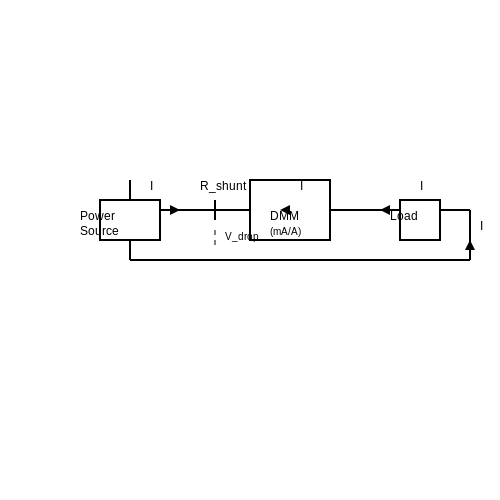
Current measurement in a digital multimeter (DMM) relies on the voltage drop across a known shunt resistor, governed by Ohm's Law:
where I is the current, V is the voltage drop, and R is the shunt resistance. For DC measurements, the DMM detects the polarity and magnitude of the voltage drop, while AC measurements require RMS conversion for accurate readings.
Measurement Modes and Shunt Resistance
DMMs typically offer multiple current ranges (e.g., 200 µA to 10 A) by switching between internal shunt resistors. The effective resistance Rshunt is given by:
where VFSD is the full-scale deflection voltage (usually 200 mV) and IFSD is the full-scale current for the selected range. Lower current ranges use higher shunt resistances to maintain sensitivity.
AC Current Measurement and True RMS
For AC current, the DMM must compute the root mean square (RMS) value to account for waveform variations. The RMS current IRMS for a periodic signal i(t) is:
Advanced DMMs use dedicated RMS-to-DC converters (e.g., Analog Devices AD737) for accurate measurements of non-sinusoidal waveforms.
Practical Considerations
- Series Connection: Current must be measured in series with the load, breaking the circuit to insert the DMM.
- Burden Voltage: The voltage drop across the shunt resistor (I × Rshunt) can affect circuit operation, especially in low-voltage systems.
- Fuse Protection: High-current ranges (e.g., 10 A) often include fast-acting fuses to protect the meter from overloads.
Advanced Techniques
For high-frequency or high-current applications beyond a DMM's capabilities, consider:
- Current Probes: Hall-effect or Rogowski coils for non-invasive measurements.
- Precision Shunts: External low-inductance shunts with four-terminal Kelvin connections.
- Oscilloscope Integration: Using a current probe with an oscilloscope for time-domain analysis.
Error Sources and Mitigation
Common error sources include:
- Shunt Heating: Power dissipation (I²R) can alter resistance values.
- Frequency Response: Limited bandwidth (typically <1 kHz for basic DMMs) attenuates high-frequency components.
- Phase Errors: In AC measurements, phase mismatch between voltage and current affects power calculations.
2.3 Measuring Resistance
Fundamentals of Resistance Measurement
Resistance measurement using a digital multimeter (DMM) relies on the principle of Ohm's Law, which states that the current (I) through a conductor between two points is directly proportional to the voltage (V) across those points and inversely proportional to the resistance (R):
Modern DMMs measure resistance by sourcing a known current through the component under test and measuring the resulting voltage drop. The internal circuitry then calculates the resistance using the above relationship. High-precision measurements require accounting for lead resistance, thermoelectric effects, and noise.
Measurement Techniques
For accurate resistance measurement, follow these steps:
- Disconnect power — Ensure the circuit is de-energized to prevent damage to the DMM.
- Select the appropriate range — Auto-ranging DMMs simplify this, but manual ranging may be necessary for high-precision measurements.
- Null lead resistance — Use the relative mode (Δ) to subtract lead resistance when measuring low resistances (< 1 Ω).
- Minimize noise — Use shielded cables and avoid high electromagnetic interference environments.
Four-Wire Kelvin Measurement
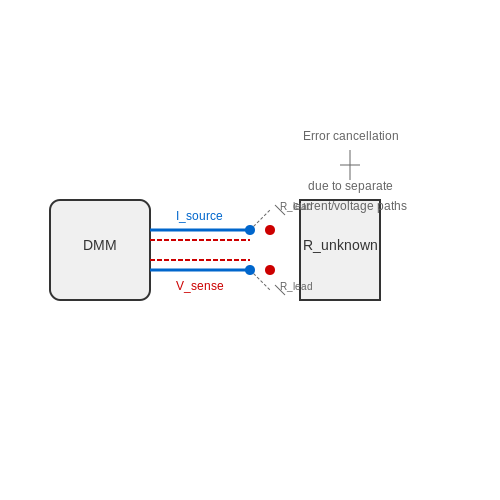
For resistances below 1 Ω, the four-wire (Kelvin) method eliminates lead resistance errors by separating current injection and voltage sensing paths:
This technique is essential in precision applications such as shunt resistor calibration and semiconductor characterization.
Nonlinear and Reactive Components
When measuring nonlinear components (e.g., diodes, thermistors) or reactive elements (e.g., inductors, capacitors), the DMM's DC excitation may not yield meaningful results. Instead:
- Use an LCR meter for impedance measurements at specific frequencies.
- Apply a small test current to avoid heating effects in sensitive components.
Practical Considerations
Resistance measurements are affected by:
- Temperature — Many materials exhibit temperature-dependent resistivity (e.g., metals increase resistance with temperature, while semiconductors decrease).
- Contact resistance — Poor probe contact introduces additional resistance.
- Dielectric absorption — In high-impedance circuits (>1 MΩ), residual charge can distort readings.
For high-resistance measurements (>10 MΩ), use guarded connections and allow sufficient settling time.
Advanced Applications
Resistance measurements extend beyond simple component testing:
- Material characterization — Sheet resistance measurements in thin-film deposition.
- Fault detection — Insulation resistance testing in high-voltage systems.
- Biological impedance — Skin resistance measurements in medical diagnostics.
2.4 Continuity Testing
Fundamentals of Continuity Testing
Continuity testing is a method for verifying the integrity of electrical connections by measuring the resistance between two points. A digital multimeter (DMM) in continuity mode applies a small test voltage (typically 1–5 V) and measures the resulting current flow. If the resistance is below a threshold (usually 10–50 Ω), the DMM emits an audible beep, indicating a continuous path. The underlying principle is governed by Ohm's Law:
where R is resistance, V is the test voltage, and I is the measured current. Advanced DMMs may use pulsed DC or AC signals to minimize noise interference in high-impedance circuits.
Practical Implementation
When performing continuity testing, the DMM's internal circuitry compares the measured resistance against a preset threshold. The beep frequency or tone may vary depending on the resistance magnitude, providing additional diagnostic information. For example:
- Solid connection: Resistance < 5 Ω, continuous beep.
- Degraded connection: Resistance 5–50 Ω, intermittent beep.
- Open circuit: Resistance > threshold, no beep.
In precision applications, the test current must be limited to avoid damaging sensitive components. High-end DMMs allow adjustable thresholds and current limits to accommodate different materials (e.g., copper vs. aluminum traces).
Advanced Considerations
Continuity testing in complex circuits requires accounting for parallel paths and capacitive/inductive coupling. A four-wire Kelvin measurement may be necessary to eliminate lead resistance errors in low-ohm applications. The time constant τ of the circuit under test can affect readings:
where C is capacitance and L is inductance. For high-frequency circuits, a time-domain reflectometer (TDR) may provide more accurate discontinuity localization than a standard DMM.
Case Study: PCB Trace Verification
In a multilayer PCB, continuity testing verifies via connections between layers. A 0.1 mm trace with 1 oz copper has a theoretical resistance of ~0.5 Ω/cm. Measured deviations exceeding 10% may indicate microfractures or plating voids. Temperature coefficients (~0.4%/°C for copper) must be considered in extreme environments.
The diagram illustrates a typical continuity test setup for PCB traces, where probes A and B must contact exposed test points while avoiding adjacent conductive elements that could create parallel paths.
2.5 Diode Testing
Fundamentals of Diode Testing
Diode testing using a digital multimeter (DMM) relies on the fundamental principle of semiconductor junction behavior. A diode conducts current in the forward-biased condition (anode positive relative to cathode) and blocks current in reverse bias. The DMM applies a small test voltage (typically 2–3 V) and measures the resulting current to determine the diode's health.
Forward Voltage Drop Measurement
When testing a diode in forward bias, the DMM measures the forward voltage drop (VF), which is characteristic of the diode material:
where:
- n = ideality factor (1 for ideal diodes, ~1–2 for real diodes)
- k = Boltzmann constant (1.38 × 10⁻²³ J/K)
- T = temperature in Kelvin
- q = electron charge (1.6 × 10⁻¹⁹ C)
- IF = forward current
- IS = reverse saturation current
For silicon diodes, expect VF ≈ 0.5–0.7 V; for Schottky diodes, ≈0.2–0.3 V.
Reverse Leakage Current Estimation
In reverse bias, the DMM measures leakage current (IR). A healthy diode exhibits minimal leakage (nA to µA range). The DMM computes an equivalent resistance:
where Vtest is the DMM's applied reverse voltage. A reading of "OL" (overload) indicates acceptable leakage, while low resistance suggests a shorted diode.
Practical Testing Procedure
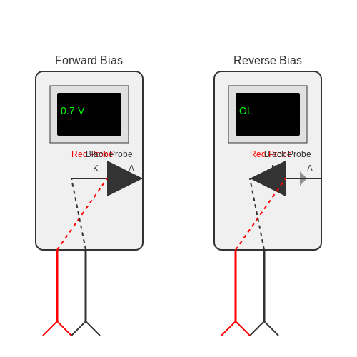
- Set the DMM to diode test mode (symbol: ⎓).
- Connect the red probe to the anode, black to the cathode for forward bias.
- Record VF. No reading indicates an open diode.
- Reverse probes to test leakage. "OL" confirms proper blocking.
Advanced Diagnostics
For Zener diodes, the breakdown voltage (VZ) can be measured by:
- Using a DMM with a variable test voltage (high-end models)
- Observing the voltage at which current begins to flow in reverse
For LEDs, the DMM may illuminate the LED dimly during forward-bias testing due to limited test current (1–2 mA).
Common Pitfalls
- In-circuit testing: Parallel components may distort readings. Isolate the diode for accurate results.
- High-power diodes: DMM test currents may be insufficient to fully turn on high-current diodes, yielding false high VF.
- Temperature dependence: VF decreases by ≈2 mV/°C for silicon diodes.
Case Study: Identifying Faulty Diodes
A diode with VF = 0 V is shorted; one with VF = "OL" in forward bias is open. Intermediate values (e.g., 0.3 V for a silicon diode) suggest degradation or a counterfeit component.
3. Capacitance Measurement
3.1 Capacitance Measurement
Fundamentals of Capacitance Measurement
Capacitance is a measure of a component's ability to store charge per unit voltage, defined as:
where C is capacitance in farads (F), Q is charge in coulombs (C), and V is voltage (V). A digital multimeter (DMM) measures capacitance by applying a known current and measuring the resulting voltage ramp rate, exploiting the time-domain relationship:
Measurement Techniques in Digital Multimeters
Modern DMMs employ one of two primary methods for capacitance measurement:
- Charge/Discharge Method: The meter applies a constant current to charge the capacitor, then measures the time required to reach a threshold voltage.
- AC Impedance Method: The meter applies a small AC signal (typically 1 kHz) and measures the resulting impedance magnitude and phase angle.
The charge/discharge method is more common in handheld DMMs due to its simpler implementation. The measured capacitance is derived from:
where I is the charging current, Δt is the measured charging time, and ΔV is the voltage change.
Practical Measurement Considerations
Parasitic Effects
When measuring small capacitances (below 100 pF), parasitic capacitances in test leads and fixture become significant. The measurement error δC can be modeled as:
where Cstray represents stray capacitances and Clead are lead capacitances. For accurate measurements below 1 nF, use shielded cables and minimize lead lengths.
Dielectric Absorption
In high-quality capacitors (e.g., film or ceramic types), dielectric absorption causes measurement errors due to slow charge redistribution. The effect is quantified by the dielectric absorption constant DA:
where Vreappearing is the voltage that reappears across the capacitor after a brief discharge.
Advanced Measurement Techniques
For precision measurements (better than 0.1% accuracy), bridge methods are preferred. The Schering bridge configuration balances unknown capacitance Cx against known standards:
where Cs is a standard capacitor, and R3, R4 are precision resistors. Modern auto-balancing bridges in laboratory-grade LCR meters achieve accuracies up to 0.01%.
Real-World Applications
Capacitance measurement is critical in:
- Quality control of multilayer ceramic capacitors (MLCCs) where C must be verified within ±1% tolerance
- Characterizing semiconductor junctions where depletion capacitance reveals doping profiles
- Monitoring electrochemical double-layer capacitors (supercapacitors) where capacitance indicates state of health
For high-voltage capacitors, always discharge the component before measurement. The stored energy E in joules is:

3.2 Frequency Measurement
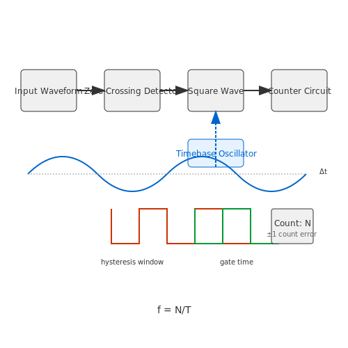
Frequency measurement with a digital multimeter (DMM) relies on counting the number of signal cycles within a known time interval. Most DMMs employ a zero-crossing detector or comparator-based triggering to convert the input waveform into a square wave, which is then processed by a counter circuit. The frequency f is calculated as:
where N is the number of cycles counted and T is the gate time. Advanced DMMs use reciprocal counting, measuring the period between successive zero-crossings and computing frequency as its inverse:
Accuracy Considerations
The accuracy of frequency measurement depends on:
- Timebase stability: Crystal oscillator drift (±1–50 ppm) introduces error.
- Trigger hysteresis: Noise immunity requires 10–30 mV threshold windows.
- Signal conditioning: High-impedance inputs (1–10 MΩ) may attenuate low-voltage signals.
For signals below 100 mVpp, an external amplifier or AC coupling is recommended. High-frequency measurements (>100 kHz) require attention to probe capacitance (typically 50–150 pF), which forms a low-pass filter with the source impedance:
Practical Implementation
Modern DMMs integrate frequency measurement through:
- Direct counting (0.1 Hz–10 MHz range)
- Period averaging (improves resolution for low frequencies)
- FFT-based analysis (in high-end models like Fluke 289)
For precise measurements, synchronize the gate time with the signal period to avoid ±1 count error. The relative error ε is bounded by:
where Δτ/τ is the timebase error. At 1 MHz with a 1-second gate time, this yields ε ≈ ±1 ppm with a high-stability oscillator.
Advanced Techniques
For non-sinusoidal waveforms, DMMs may employ:
- Schmitt trigger conditioning to handle distorted signals
- Harmonic rejection filters for power line measurements
- Phase-locked loops (PLLs) in RF-capable multimeters
When measuring PWM signals, ensure the DMM's bandwidth exceeds the rise time requirements. A 100 kHz PWM signal with 100 ns edges needs a bandwidth >3.5 MHz to avoid slew-rate-induced errors:
3.3 Temperature Measurement
Thermocouple Principles and Seebeck Effect
Digital multimeters measure temperature using thermocouples, which rely on the Seebeck effect: a voltage gradient forms when two dissimilar metals are joined and subjected to a thermal gradient. The output voltage V is proportional to the temperature difference ΔT between the junction (TJ) and the reference point (Tref). The relationship is given by:
where α and β are material-dependent Seebeck coefficients. For small ranges, higher-order terms are negligible, simplifying to V ≈ αΔT.
Cold Junction Compensation (CJC)
Since thermocouples measure relative temperature, the multimeter must compensate for the reference junction temperature (typically the instrument’s terminal block). Modern DMMs use an integrated thermistor or RTD to measure Tref and adjust readings accordingly. The corrected temperature TJ is computed as:
Practical Considerations
- Thermocouple Types: Type K (chromel-alumel) is common due to its wide range (−200°C to +1350°C) and linearity. Type T (copper-constantan) offers higher precision for cryogenic applications.
- Noise Mitigation: Twisted-pair cables and shielded connectors minimize electromagnetic interference, which can distort low-voltage thermocouple signals (typically 10–100 µV/°C).
- Calibration: Regular calibration against a known reference (e.g., ice bath or dry block calibrator) ensures accuracy, especially for sub-degree resolution.
Advanced Techniques
For high-precision applications, multichannel DMMs can average multiple thermocouple readings or implement nonlinear correction algorithms to account for Seebeck coefficient variations across temperature ranges. Some instruments support NIST-traceable calibration curves for specific thermocouple types.
Error Sources and Mitigation
- Thermal Shunting: Poor thermal contact between the probe and target introduces lag. Use thermally conductive paste for solid surfaces.
- Ground Loops: Floating measurements or isolation amplifiers prevent stray currents from affecting readings.
- Drift: Aging thermocouples develop inhomogeneities; replace probes if calibration shifts exceed specifications.

3.4 Using Hold and Relative Modes
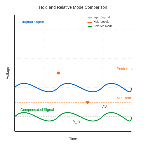
Hold Mode: Freezing Measurements for Analysis
The Hold function in a digital multimeter (DMM) captures and retains the current measurement value on the display, regardless of subsequent changes in the input signal. This is particularly useful in scenarios where:
- Measuring rapidly fluctuating signals (e.g., ripple voltage in power supplies).
- Recording peak values in transient events (e.g., inrush current in motor startups).
- Working in environments where the display is difficult to read in real-time (e.g., low-light or high-vibration conditions).
When activated, the DMM samples the input signal and latches the value into its display memory. The analog-to-digital converter (ADC) continues to process new measurements internally, but the displayed value remains static until Hold is deactivated. Some advanced DMMs offer peak-hold or min/max-hold modes, which track and display the highest or lowest recorded values over a period.
Relative Mode: Nulling Baseline Offsets
The Relative mode (often denoted as Δ or REL) allows the user to establish a reference baseline measurement and subsequently display only the difference from that baseline. Mathematically, if the baseline measurement is Vref, subsequent measurements Vm are displayed as:
This mode is indispensable in applications such as:
- Precision resistance measurements, where lead resistance must be nulled out.
- Small voltage differentials in Wheatstone bridge circuits.
- Thermocouple measurements, where ambient temperature effects need compensation.
When Relative mode is engaged, the DMM stores the current reading as Vref and resets the display to zero. All subsequent measurements are offset by this value. High-precision DMMs often combine Relative mode with high-resolution ADCs (e.g., 6½-digit) to resolve microvolt-level differences.
Practical Implementation Considerations
In high-impedance circuits, the act of pressing the Hold or Relative buttons can introduce noise due to stray capacitance. To mitigate this:
- Use shielded test leads when measuring signals below 1 mV.
- Enable input buffering if the DMM supports it, reducing input current leakage.
- For AC measurements, ensure the DMM's sampling rate exceeds the signal's highest frequency component by at least 5× to avoid aliasing.
Some DMMs implement these modes digitally (post-ADC), while others use analog techniques. For instance, the Fluke 87V employs a dedicated analog subtractor circuit for Relative mode, preserving the full ADC resolution. In contrast, budget DMMs often perform the subtraction digitally, which can quantize small differences.
Case Study: Thermocouple Compensation
When measuring a Type K thermocouple with a DMM, the Relative mode nulls the cold junction compensation voltage. If the thermocouple outputs 12.347 mV at 250°C and the cold junction is at 25°C (contributing 1.000 mV), engaging Relative mode at 25°C effectively subtracts the 1.000 mV offset, displaying only the 11.347 mV proportional to the temperature differential.
4. Electrical Safety Guidelines
4.1 Electrical Safety Guidelines
High-Voltage Hazards and Mitigation
When working with a digital multimeter (DMM) in high-voltage environments (>50 V AC or >120 V DC), the risk of arc flash, insulation breakdown, and capacitive coupling increases significantly. The transient energy E during a fault can be modeled as:
where C is stray capacitance, V is the potential difference, and I is fault current. For example, a 1 pF stray capacitance at 10 kV stores 50 mJ—enough to cause severe burns.
Personal Protective Equipment (PPE)
- Category-rated tools: Use DMMs and probes rated for CAT III 1000 V or CAT IV 600 V per IEC 61010-1.
- Insulated gloves: Class 00 (500 V AC) minimum, with leather protectors for arc flash protection.
- Face shields: Required for voltages exceeding 240 V due to plasma formation risks.
Measurement Best Practices
Always connect the ground lead first in high-impedance circuits to avoid floating potentials. For current measurements, ensure the DMM's internal shunt resistance Rshunt won't exceed the circuit's Thévenin equivalent resistance:
where Voc is open-circuit voltage and Isc is short-circuit current. A 10:1 ratio is recommended.
Grounding and Isolation
In mixed-signal systems, ground loops introduce measurement errors and safety risks. The ground potential difference ΔVgnd between two points can induce noise currents:
where Zloop is the loop impedance. Optical isolators or differential probes are preferred for >30 V measurements.
DMM Internal Protection Limits
All DMMs have a voltage burden effect in current-measurement mode. The burden voltage Vb is given by:
Exceeding the manufacturer's specified burden (typically 200–500 mV) may damage the meter or circuit. For example, a 10 A current through a 50 mΩ shunt produces 500 mV—the limit for many DMMs.
Transient Protection
Fast transients (e.g., inductive kickback) require TVS diodes or gas discharge tubes in the DMM input stage. The let-through energy ETVS must satisfy:
where L is circuit inductance. A 1 mH inductor discharging 1 A requires a TVS rated for at least 0.5 mJ.
4.2 Proper Probe Handling
Electrical Contact Integrity
Ensuring low-resistance contact between the probe tip and the measurement point is critical for accurate readings. The contact resistance (Rcontact) can introduce errors, particularly in high-impedance circuits. For a typical digital multimeter (DMM) with input impedance of 10 MΩ, even a contact resistance of 1 kΩ can lead to a 0.01% error in voltage measurements. However, in low-voltage or high-current scenarios, this error becomes non-negligible.
To minimize Rcontact, apply firm but controlled pressure when probing. Oxidation or contamination on the probe tip increases resistance—periodically clean tips with isopropyl alcohol and a fine abrasive pad.
Probe Positioning and Stability
In high-frequency measurements or circuits with fast transients, probe placement affects signal integrity. Stray capacitance and inductance from poorly positioned probes can distort readings. For example, a 10 cm unshielded probe lead can introduce ~30 pF of parasitic capacitance, significantly altering the response in RF circuits.
Safety Considerations for High-Voltage Measurements
When measuring voltages above 30 VRMS or 42 Vpeak, follow IEC 61010-1 safety standards:
- Use CAT III or CAT IV rated probes for mains voltage measurements.
- Never allow fingers to slip beyond the probe's finger guard.
- Employ alligator clips for stable connections in live circuits to avoid slips.
Thermal Effects on Probe Accuracy
Probe materials exhibit temperature-dependent resistivity. For a copper probe tip:
where α is the temperature coefficient (~0.00393/°C for copper). A 50°C rise increases resistance by ~20%, affecting low-resistance measurements. Use gold-plated probes for stable thermal performance in precision applications.
Minimizing Ground Loops
In differential measurements, improper probe grounding creates ground loops that inject noise. The induced error voltage is:
To mitigate this, connect the ground probe at a single point and use twisted-pair probe leads to reduce magnetic flux coupling.
4.3 Avoiding Common Mistakes
Incorrect Range Selection
A frequent error when using digital multimeters (DMMs) is selecting an inappropriate measurement range. If the range is set too low for the measured quantity, the meter may display an overload condition or, worse, sustain damage. Conversely, selecting a range that is too high reduces measurement resolution and accuracy. For instance, measuring a 3.3V signal on a 20V range instead of the available 4V range introduces unnecessary quantization error. Modern auto-ranging DMMs mitigate this issue but may exhibit slower response times.
Ignoring Burden Voltage in Current Measurements
When measuring current, the DMM introduces a small series resistance (burden voltage), altering the circuit's behavior. The burden voltage Vb can be calculated as:
where Rint is the meter's internal resistance in current mode. For precise measurements, compensate for this effect by either:
- Using a DMM with low burden voltage specification
- Calculating the corrected current as Iactual = Imeasured × (1 + Rint/Rload)
AC/DC Coupling Confusion
Many advanced DMMs offer both AC and DC measurement modes. A common mistake is using AC coupling when DC measurements are required, or vice versa. This is particularly critical when measuring:
- Ripple voltage on DC power supplies (requires AC coupling)
- True RMS values of complex waveforms
- DC offsets in AC signals
Probe Placement Errors
Improper probe placement introduces measurement artifacts through:
- Ground loops when using separate ground references
- Capacitive coupling in high-frequency measurements
- Thermal voltages at dissimilar metal junctions (Seebeck effect)
For microvolt-level measurements, use gold-plated probes and maintain isothermal conditions.
Overlooking Input Impedance Effects
The DMM's input impedance (typically 10MΩ for voltage measurements) forms a voltage divider with the source impedance. The resulting measurement error ε is:
When measuring high-impedance circuits (e.g., pH electrodes, piezoelectric sensors), use a DMM with >1GΩ input impedance or buffer amplifiers.
Failure to Account for Crest Factor
When measuring non-sinusoidal waveforms, the crest factor (ratio of peak to RMS value) affects measurement accuracy. Most DMMs specify accuracy only for crest factors ≤3:1. For pulsed or complex waveforms:
- Verify the DMM's crest factor specification
- Use true RMS meters with high crest factor capability (>10:1)
- Consider specialized instruments for high-frequency components
Neglecting Calibration and Temperature Effects
DMM accuracy specifications assume:
- Proper calibration within the last 6-12 months
- Operation within the specified temperature range (typically 18-28°C)
Outside these conditions, additional errors accumulate according to:
where α is the temperature coefficient (usually ppm/°C) and Tref is the reference temperature.
5. Diagnosing Common Issues
5.1 Diagnosing Common Issues
Intermittent Connections and Signal Integrity
Intermittent connections often manifest as erratic readings or sudden drops in measured values. These issues arise due to poor contact resistance, oxidation, or mechanical stress on test leads. To diagnose, monitor the multimeter's display while gently flexing the leads near their terminations. A high-quality multimeter with a bar graph or analog-style response can reveal transient fluctuations more effectively than a purely digital display.
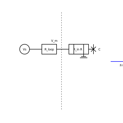
Ground Loops and Stray Voltages
When measuring low-voltage signals in grounded systems, ground loops introduce erroneous offsets. The multimeter's input impedance (typically 10 MΩ) forms a voltage divider with the loop resistance. For a ground loop resistance Rloop and source voltage Vs, the measured voltage Vm is:
To mitigate, use differential measurements or isolate the ground reference. High-end multimeters offer guarded inputs to reject common-mode noise.
Overload Recovery and Saturation
After exposure to voltages beyond the multimeter's range, the analog front-end may saturate, causing prolonged recovery times. For instance, applying 100 V to a 20 V range can saturate the input amplifier for milliseconds to seconds, depending on the design. Verify recovery by observing the settling time when switching from an overload condition to a known reference voltage.
Thermal EMF Effects
Thermoelectric voltages at dissimilar metal junctions (e.g., test lead alloys) introduce DC offsets. For copper-constantan junctions, the Seebeck coefficient is approximately 40 µV/°C. When measuring low resistances (< 1 Ω), these effects dominate. Use four-wire Kelvin measurements and zero the multimeter before testing to cancel thermal EMF.
Frequency Response Limitations
Digital multimeters exhibit roll-off in AC measurements due to bandwidth constraints. The -3 dB bandwidth fc of a typical multimeter's input filter is:
where R and C are the input network components. For accurate RMS measurements beyond 1 kHz, verify the multimeter's specified bandwidth or use a true-RMS converter.
Battery and Self-Discharge Effects
Low battery voltage affects the multimeter's reference stability, particularly in precision models. The internal voltage reference drift ΔVref follows:
where α is the regulator's line regulation coefficient. Replace batteries when the low-battery indicator activates, and avoid leaving the multimeter in resistance-measurement mode, which drains power through the test leads.
5.2 Calibrating Your Multimeter
Fundamentals of Calibration
Calibration ensures that a multimeter's measurements align with traceable standards, typically referenced to the International System of Units (SI). A digital multimeter (DMM) relies on internal voltage references, precision resistors, and analog-to-digital converter (ADC) linearity. Over time, component aging, thermal drift, and mechanical stress introduce errors, necessitating periodic calibration.
where α is the gain error (percentage of reading) and β is the offset error (fixed value). Calibration corrects both terms by adjusting the DMM's firmware or hardware trimmers.
Traceability and Standards
Calibration requires a reference source with 4–10× better accuracy than the DMM under test. Common standards include:
- Fluke 5520A Multi-Product Calibrator (0.0015% DC voltage accuracy)
- Josephson Voltage Standards (quantum-accurate, used by NIST)
- Precision shunt resistors (for current measurements, 0.002% tolerance)
Procedure for DC Voltage Calibration
For a 6.5-digit DMM (e.g., Keysight 34401A):
- Connect the DMM to a calibrated voltage source (e.g., 10.0000V).
- Access calibration mode via manufacturer-specific key sequences.
- Input the reference value and allow the DMM to adjust its gain coefficients.
- Verify linearity at 1V, 5V, and 10V points using a least-squares fit:
AC and Resistance Calibration
AC calibration requires a precision AC source with known THD (<0.1%) and frequency stability (±1ppm). For resistance, use a 4-wire Kelvin connection to eliminate lead resistance errors:
Environmental Considerations
Calibration validity depends on:
- Temperature: Perform at 23°C ±1°C (per IEC 60751)
- Warm-up time: ≥1 hour for thermal equilibrium
- EMI: Shield against >3V/m RF interference
Documentation and Compliance
Maintain records per ISO/IEC 17025, including:
- As-found/as-left data
- Measurement uncertainty budget (typically ±(0.005% + 2μV) for DCV)
- Traceability chain to NIST or equivalent NMIs
5.3 Battery Replacement and Care
Battery Chemistry and Multimeter Power Requirements
Most digital multimeters (DMMs) operate on standard 9V alkaline or lithium batteries, though some high-precision benchtop models may use AA or AAA cells. The choice of battery impacts not only operational lifespan but also measurement stability, particularly in sensitive DC voltage and resistance measurements. Lithium batteries, while more expensive, exhibit a flatter discharge curve, reducing voltage drift errors in precision measurements:
where \( \Delta V_{\text{error}} \) is the reference voltage drift over time \( \Delta t \). Lithium cells typically maintain \( \frac{\partial V_{\text{ref}}}{\partial t} < 0.1\%/\text{month} \) compared to 0.5-1%/month for alkaline.
Battery Replacement Protocol
Follow this procedure to minimize measurement discontinuity and prevent damage:
- Power-down sequence: Turn the rotary switch to OFF, disconnect all test leads, and wait 30 seconds for internal capacitors to discharge.
- ESD precautions: Ground yourself and the DMM chassis before accessing the battery compartment to prevent electrostatic discharge damage to sensitive ICs.
- Polarity verification: Confirm battery orientation against the compartment diagram. Reverse insertion can trigger protection circuits, requiring a full reset.
Battery Performance Monitoring
Modern DMMs implement battery health indicators through:
- Load voltage testing (measuring voltage under 10-20mA load)
- Coulomb counting (tracking total charge expended)
- Internal resistance measurement (using 4-wire Kelvin sensing)
The battery's internal resistance \( R_{\text{int}} \) follows:
where \( V_{\text{oc}} \) is open-circuit voltage and \( V_{\text{load}} \) is voltage under known load current \( I_{\text{load}} \). Replace when \( R_{\text{int}} \) exceeds 5Ω for 9V batteries.
Storage and Environmental Considerations
For long-term storage (>3 months):
- Remove batteries to prevent leakage damage from electrolyte corrosion
- Store at 40-60% charge state (3.6-3.8V/cell for lithium) to minimize aging
- Maintain temperature below 25°C to reduce self-discharge rates
The Arrhenius equation models temperature-dependent self-discharge:
where \( k \) is the discharge rate constant, \( E_a \) is activation energy (~0.5eV for lithium), and \( T \) is absolute temperature.
6. Recommended Books and Manuals
6.1 Recommended Books and Manuals
- Agilent Technologies: 34401A 6½ Digit Digital Multimeter — Agilent 34401A multimeter accessories included: Test lead kit with probe Aalligator and grabber attachments calibration certificate, test report, and power cord. Also includes CD with: IntuiLink software, IVI and VXI PnP drivers Quick start tutorial user's guide, command quick reference, service guide, and data sheet. Optional Accessories:
- Gossen MetraWatt METRALINE DM 61 Operating Instructions Manual — View and Download Gossen MetraWatt METRALINE DM 61 operating instructions manual online. Analog-Digital Multimeter. METRALINE DM 61 multimeter pdf manual download. Also for: Metraline dm 62.
- PDF Chapter-8 Electronic Measurements and Measuring Instruments — o types of meters, analog and digital meters, are utilized. The measurements of these fundamental ele trical quantitie agnetic meter mo Voltage sensing. The instruments are mostly electronic in nature, using amplifiers and semiconductor devices, such as a digital multimeter.
- PDF DM401B Multimeter-Mastering The Art of Measurement_EN.r01 — In this guide, you are going to learn how to measure DC voltage and AC voltage, AC and DC current, resistance, diodes, frequency/duty, capacitance, temperature and continuity test using DM401B 6000 Counts T-RMS Smart Digital Multimeter.
- PDF Physics 115 Electronics and Instrumentation Laboratory Manual — Introduction e electronic devices to measure and record various phenomena. Whether you need to measure temperature, light intensity, magnetic fields, humidity, charged particles, time, or st of this course is not to turn you into an electronics whiz. Rather, it is a survey course that will introduce you to the broad range of electronic device
- PDF EXPERIMENT HANDLING AND MAINTAINING A MULTIMETER - eGyanKosh — Find out the relevant specifications of the multimeter such as its operating temperature, storage temperature, battery voltage and battery life from its manual, if available.
- Digital multimeter - Free Pdf Manuals Download | ManualsLib — View and download Digital multimeter manuals for free. Digital Multimeter CP7676 instructions manual.
- PDF Model 2100 6 1/2-Digit Resolution Digital Multimeter - UC Davis — This section introduces some basic measurement functions of the Keithley Instruments Model 2100 6 1/2-Digit Resolution Digital Multimeter®. You will learn how to use the Model 2100 multimeter to measure voltage, current, resistance, frequency, period, continuity, and diode forward voltage.
- PDF USER MANUAL - RS Components — 3. Introduction Thank you for selecting the FLIR DM6x Digital Multimeter. This meter can measure up to 600V and 10A AC/DC. This device is shipped fully tested and calibrated and, with proper use, will provide years of reliable service.
- PLUSIVO DMM MANUAL Pdf Download | ManualsLib — Introduction In this guide, you are going to learn how to measure DC voltage and AC voltage, DC current, resistance, diodes, and continuity test using Digital MultiMeter (DMM).
6.2 Online Resources and Tutorials
- PDF Me 360: Fundamentals of Signal Processing, Instrumentation and Control — 6.1 Using the Digital Multimeter (DMM) for DC Voltage Measurement 6.1.1 Station Layout and Initial Setup (a) In preparation for your laboratory session, review the information on the oscilloscope, digital multimeter, function generator, and patch panel in the appendices. Note the location and organization of the controls for each instrument.
- PDF Chapter-8 Electronic Measurements and Measuring Instruments — The whole operation of the device is based on electronic components. 6.3 Multimeter Multimeter or a multitester is a measurement instrument used in electronics, which is designed to perform tasks of several measuring instruments. The voltage, current, and resistance measurements can be made using different options available in a common Multimeter.
- Solved Exercise 6.2 Measurement in a parallel circuit 1. - Chegg — Question: Exercise 6.2 Measurement in a parallel circuit 1. Connect the circuit on breadboard shown in Figure 6.6. Setup your Multimeter to read DC volts. Only close the switch when you are making measurements. Measure and record voltage across R1, R2 and voltage source in Table 6.1.
- Guide to Online Experiment 2: Electronics Lab and Multimeter Use ... — Learn how to use the Circuit Board 3. Learn how to use mulitimeter EQUIPMENT 1. EM-8656 AD/DC Electronics Lab 2. PS-3211 Wireless voltage sensor 3. PS-3212 Wireless current sensor 4, SE-8829 Student Multimeter 5. 2 Batteries 6. Wires, Resistors, and Capacitors THEORY Structure of the AC/DC Circuit Board: The structure of the Circuit Board (EM ...
- Practical Troubleshooting of Electronic Circuits for Engineers and ... — The normal range of resistors encountered in practice is 1 ohm to 10 mega-ohms. The most convenient method of checking the resistance is by using an ANALOG or DIGITAL MULTIMETER. Digital multimeter can be used to measure very low resistance values such as the contact resistance of plug and socket connectors, etc.
- How to use multimeter - Robo India || Tutorials - Learn Arduino — Robo India in this tutorial explains how to use multimeter with illustrated diagrams. 1. Multimeter: 2. Test leads ( Red and Black): 3. A complete Multimeter: 4. DC Voltage Measurement: 4.1. Connect test leads as shown in the picture. 4.2 Set rotary switch to the position as shown in the picture.
- Solved LAMAR UNIVERSITY CIRCUITS LABORATORY EXPERIMENT 2 ... - Chegg — Note that it may take up to using four resistors to obtain the desired values being asked. 2. Once you obtain the circuit for each resistor, put them on the breadboard. Then, measure the equivalent resistance of each circuit using a Multimeter (use in Ohm-meter position). Compare it to desired values.
- Multimeter - Introduction to electronic lab tools — Some also include the ability to measure AC sources and test the functionality of diodes. Be sure to have a look through the manual provided with the multimeter you own to explore its full capabilities. Ports. Before using a multimeter, you should take note of the ports being used on it (the red and black holes at the bottom of the device).
- PDF Tutorial - Building circuits & using a multimeter - University of Ottawa — Tutorial - Building circuits & using a multimeter 3 Measuring the resistance Figure 6 presents the circuit diagram for measuring the resistance value of a resistor using an ohmmeter. To use the ohmmeter, you need to select it from the list of instruments in the Digital Multimeter window (see Figure 5, it is represented by the symbol).
- PDF Mastering The Art of Measurement - Plusivo — Mastering The Art of Measurement UserGuideforthePlusivo DM301BMultimeter Mast eri ng t he A rt of Measurement (Di gi t al Mul t i met er) r. 01 www. pl usi vo. com
6.3 Manufacturer Specifications
- Fluke 117 True RMS Digital Multimeter - Jameco Electronics — The Fluke 117 multimeter is a must-have for any electrician or technician who needs a reliable and accurate multimeter to get the job done. This versatile device boasts a host of advanced features, including non-contact voltage detection, Auto Volts and LoZ functions, and integrated frequency and capacitance measurement capabilities.
- PDF FLIR MODEL DM166 Thermal Imaging Digital MultiMeter with IGMTM — 7.2 Using the Multimeter in the IGMTM mode 25 7.3 Emissivity Factors for Common Materials 25 7.4 Infrared Energy and Thermal Imaging Overview 26 8. MAINTENANCE 27 8.1 Cleaning and Storage 27 8.2 Battery Replacement 27 8.3 Fuse Replacement 27 8.4 Disposal of Electronic Waste 27 9. SPECIFICATIONS 28 9.1 General specifications 28
- Extech EX350 11 Function True RMS Digital Multimeter — his professional digital multimeter measures a total of 11 different parameters, ... EV & Electronic Multimeters Digital Multimeters. Extech EX350 11 Function True RMS Digital Multimeter. ... Extech EX350 Technical Specifications. DC Current; Type: Range: Resolution: Accuracy: μA: 400.0μA: 0.1μA: ±(0.7%+2 digits) 4000μA: 1μA: mA:
- PDF USER MANUAL True RMS Digital MultiMeter Series - Cole-Parmer — Thank you for selecting the FLIR DM6x Digital Multimeter. This meter can measure up to 600V and 10A AC/DC. This device is shipped fully tested and calibrated and, with proper use, will provide years of reliable service. Features 6000 Count (3-5/6 digits) backlit LCD with 5 reading per second update rate Auto Power OFF
- PDF User Manual ENGLISH Digital Multimeter Models 5212 & 5217 - AEMC — Digital Multimeter Models 5212/5215/5217 - User Manual 1 Thank you for purchasing an AEMC® Instruments Digital Multimeter. For the best results from your instrument and for your safety, you must read the enclosed operating instructions carefully and comply with the precautions for use. Only qualified and trained operators should use this product.
- PDF U.S.A Allied Electronics Professional True RMS Digital Multimeter — DO NOT use chemicals, cleaning solvents, or detergents. 5. USE ONLY FRESH BATTERIES OF THE RECOMMENDED SIZE AND TYPE. Remove old or weak batteries so they do not leak and damage the unit. 6. IF THE METER IS TO BE STORED FOR A LONG PERIOD OF TIME, the batteries should be removed to prevent damage to the unit. 6000 Counts OLED Digital Multimeter ...
- PDF Chapter-8 Electronic Measurements and Measuring Instruments — Digital meter is completely electronic in operation, and no mechanical components are involved in the measurements. The whole operation of the device is based on electronic components. 6.3 Multimeter Multimeter or a multitester is a measurement instrument used in electronics, which is designed to perform
- 115 Field Service Technicians Multi-meter - The Home Depot — The FLUKE 115 field technician's digital multimeter measures True-rms voltage and current with plus resistance, continuity, frequency and capacitance to meet the needs of a wide variety of field service technicians. The 115 digital multimeter offers the users one-handed operation and a backlit display.
- Cal-Chip Electronics GMC04X7R225K6R3NT - Octopart — Find the best pricing for Cal-Chip Electronics GMC04X7R225K6R3NT by comparing bulk discounts from 2 distributors. Octopart is the world's source for GMC04X7R225K6R3NT availability, pricing, and technical specs and other electronic parts.
- PDF DIGITAL MULTIMETER - HTC Instrument — 1.4.4 Do not use abrasives or solvents on the meter, use a damp cloth and mild detergent only. 1.4.5 Always set the power switch to the off position when the meter is not in use. 1.4.6 If the meter is to be stored for a long period of time, the batteries should be removed to prevent damage to the unit. 2. DESCRIPTION 2.1 NAMES OF COMPONENTS