Solar Panel Circuits
1. Basic Principles of Photovoltaic Energy Conversion
1.1 Basic Principles of Photovoltaic Energy Conversion
Fundamental Physics of Photovoltaic Effect
The photovoltaic effect arises from the interaction of photons with semiconductor materials, generating electron-hole pairs. When photons with energy Ephoton ≥ Eg (where Eg is the bandgap energy) strike a semiconductor, they excite electrons from the valence band to the conduction band. This creates mobile charge carriers that can be separated by an internal electric field, typically formed at a p-n junction.
where h is Planck's constant (6.626 × 10⁻³⁴ J·s), c is the speed of light (3 × 10⁸ m/s), and Eg is in electron volts (eV). For silicon (Eg ≈ 1.1 eV), this yields a cutoff wavelength of approximately 1100 nm.
Charge Separation and Collection
The built-in potential at the p-n junction creates a depletion region where the electric field drives electrons toward the n-side and holes toward the p-side. This separation process is governed by:
where Jdrift is the drift current density, q is the elementary charge, μn and μp are electron and hole mobilities, n and p are carrier concentrations, and E is the electric field strength.
Current-Voltage Characteristics
The ideal solar cell I-V relationship is derived from the Shockley diode equation modified for photocurrent:
where Iph is the photogenerated current, I0 is the reverse saturation current, n is the ideality factor, k is Boltzmann's constant, and T is temperature in Kelvin.
Key Performance Parameters
The efficiency (η) of a solar cell is determined by:
where Voc is open-circuit voltage, Isc is short-circuit current, and FF is fill factor. The maximum theoretical efficiency for a single-junction solar cell under standard test conditions (AM1.5 spectrum, 1000 W/m2) is limited to ~33% (Shockley-Queisser limit).
Loss Mechanisms
Practical solar cells exhibit several loss mechanisms:
- Optical losses: Reflection (~4% at air/glass interface) and incomplete absorption
- Recombination losses: Radiative, Auger, and Shockley-Read-Hall recombination
- Resistive losses: Series resistance in contacts and bulk material
- Spectral mismatch: Sub-bandgap and above-bandgap photon energy waste
Advanced Concepts
For high-efficiency designs, several advanced principles become critical:
- Surface passivation to reduce recombination (e.g., SiO2/SiNx layers)
- Light trapping through textured surfaces and back reflectors
- Selective contacts to minimize carrier recombination at interfaces
- Bandgap engineering in multi-junction cells
1.2 Key Components in Solar Panel Circuits
Photovoltaic Cells
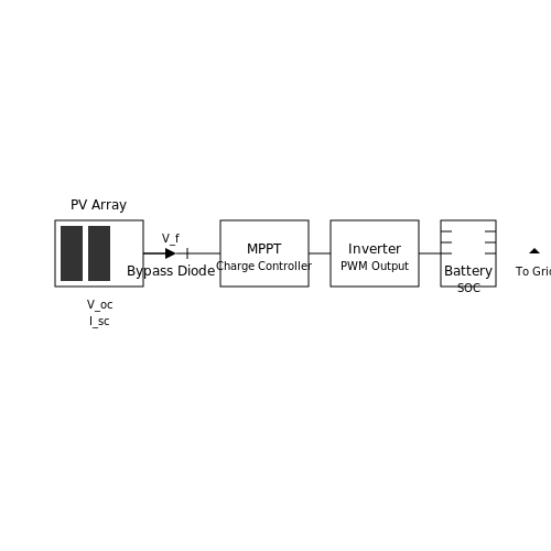
The fundamental building block of any solar panel circuit is the photovoltaic (PV) cell, which converts incident photons into electrical energy via the photovoltaic effect. A PV cell operates as a p-n junction semiconductor, where electron-hole pairs are generated upon photon absorption. The open-circuit voltage (Voc) and short-circuit current (Isc) are critical parameters:
where n is the ideality factor, IL is the light-generated current, and η(λ) is the quantum efficiency at wavelength λ.
Bypass Diodes
Bypass diodes mitigate power loss due to partial shading or cell mismatch. When a cell's output drops below the forward bias voltage of the diode (typically 0.6–0.7V for silicon), the diode provides an alternative current path. The power dissipation in a bypass diode is given by:
where Vf is the forward voltage and Rs is the series resistance. Schottky diodes are preferred for their low Vf.
Charge Controllers
Maximum Power Point Tracking (MPPT) charge controllers optimize energy transfer by dynamically adjusting the load impedance to match the PV array's peak power voltage (Vmp). The MPPT algorithm solves:
Perturb-and-observe (P&O) and incremental conductance (INC) are common MPPT methods, with efficiencies exceeding 97% in modern implementations.
Inverters
Grid-tied systems require inverters to convert DC to AC power. The total harmonic distortion (THD) must comply with IEEE 1547 standards (<5% for individual harmonics). The output voltage waveform is synthesized using pulse-width modulation (PWM):
where D(t) is the duty cycle. Silicon carbide (SiC) MOSFETs are increasingly used for high-frequency switching (>20 kHz) with reduced losses.
Energy Storage
Lithium-ion batteries dominate due to high energy density (>200 Wh/kg) and cycle life (>5000 cycles at 80% depth of discharge). The state of charge (SOC) is estimated via Coulomb counting:
where Cn is the nominal capacity. Battery management systems (BMS) maintain cell balancing within ±10 mV.
Types of Solar Panels and Their Electrical Characteristics
Monocrystalline Silicon (Mono-Si) Panels
Monocrystalline solar panels are fabricated from single-crystal silicon ingots grown via the Czochralski process. Their high purity results in superior charge carrier mobility, leading to efficiencies typically between 18% and 22%. The open-circuit voltage (Voc) for a standard 60-cell Mono-Si panel under standard test conditions (STC) ranges from 36V to 40V, while the short-circuit current (Isc) falls between 8A and 9A. Their temperature coefficient for power (γ) is approximately -0.35%/°C, making them less susceptible to efficiency losses at elevated temperatures compared to polycrystalline panels.
Polycrystalline Silicon (Poly-Si) Panels
Polycrystalline panels are manufactured by casting molten silicon into square molds, resulting in multiple crystal domains. The presence of grain boundaries increases charge recombination, reducing efficiency to 15%–17%. A typical 60-cell Poly-Si panel exhibits a Voc of 32V–36V and Isc of 8.5A–9.5A. The temperature coefficient for power is slightly worse (-0.40%/°C to -0.45%/°C) due to higher defect density. However, their lower production cost makes them economically viable for large-scale installations where space is not a constraint.
Thin-Film Solar Technologies
Amorphous Silicon (a-Si)
Amorphous silicon panels utilize non-crystalline silicon deposited in thin layers (~1 µm) on substrates like glass or metal. Their disordered atomic structure leads to a wider bandgap (~1.7 eV) compared to crystalline silicon, resulting in better performance under low-light conditions but lower efficiencies (6%–10%). The Staebler-Wronski effect causes light-induced degradation, reducing output by 10%–15% during initial exposure.
Cadmium Telluride (CdTe)
CdTe thin-film panels achieve efficiencies of 10%–12% in commercial modules, with laboratory cells exceeding 22%. Their direct bandgap of 1.45 eV provides strong light absorption, allowing active layers as thin as 2–3 µm. A key advantage is their superior temperature coefficient (-0.25%/°C), making them ideal for hot climates. However, the toxicity of cadmium necessitates specialized recycling processes.
Copper Indium Gallium Selenide (CIGS)
CIGS panels combine a tunable bandgap (1.0–1.7 eV) with high absorption coefficients (>105 cm-1). Record lab efficiencies exceed 23%, with commercial modules reaching 13%–15%. Their flexible substrates enable building-integrated photovoltaics (BIPV) applications. The heterojunction structure creates a built-in electric field that enhances charge collection.
Tandem and Multi-Junction Cells
Multi-junction cells stack multiple semiconductor layers with decreasing bandgaps to capture a broader solar spectrum. A typical InGaP/GaAs/Ge triple-junction cell achieves 30%–32% efficiency under concentrated sunlight. The current matching condition for series-connected subcells is critical:
Quantum dot and perovskite-based tandem cells are emerging as promising alternatives, with theoretical Shockley-Queisser limits exceeding 40%. Recent developments in 2D/3D perovskite heterostructures have demonstrated improved stability against moisture and heat degradation.
Electrical Parameter Comparison
The following table summarizes key electrical characteristics under STC (1000 W/m2, AM1.5, 25°C):
| Technology | Efficiency (%) | Voc (V) | Isc (A) | FF (%) | Temp. Coeff. (%/°C) |
|---|---|---|---|---|---|
| Mono-Si | 18–22 | 0.60–0.65 | 8.0–9.0 | 75–82 | -0.35 |
| Poly-Si | 15–17 | 0.55–0.60 | 8.5–9.5 | 72–78 | -0.42 |
| CdTe | 10–12 | 0.85–0.95 | 6.5–7.5 | 70–75 | -0.25 |
| CIGS | 13–15 | 0.70–0.75 | 7.0–8.0 | 75–80 | -0.30 |
2. Calculating Power Requirements and Panel Sizing
2.1 Calculating Power Requirements and Panel Sizing
Fundamentals of Solar Power Calculation
The instantaneous electrical power output P of a solar panel under ideal conditions is given by:
where Voc is the open-circuit voltage, Isc is the short-circuit current, and FF is the fill factor (typically 0.7-0.85 for commercial panels). However, real-world conditions require accounting for several derating factors:
where PSTC is the power under Standard Test Conditions (1000 W/m² irradiance, 25°C cell temperature, AM1.5 spectrum), and η terms represent efficiency factors for temperature (0.85-0.95), dirt accumulation (0.90-0.98), module mismatch (0.95-0.99), and inverter losses (0.92-0.97).
Daily Energy Requirements
For system sizing, we first calculate the daily load energy requirement Eload:
where Pi is the power of each load and ti is its daily usage time. For example, a 100W load running 5 hours/day consumes 500Wh.
Peak Sun Hours and Panel Sizing
The required panel array power Parray is determined by:
where PSH (Peak Sun Hours) represents the equivalent hours of full sun intensity at the installation location (typically 3-6 hours depending on geography and season), and ηsystem accounts for all efficiency losses (typically 0.65-0.75).
Temperature Derating
Solar cell efficiency decreases with temperature, following:
where γ is the temperature coefficient (typically -0.3% to -0.5%/°C for silicon), Tcell is the actual operating temperature, and TSTC = 25°C. The cell temperature can be estimated from ambient temperature Tamb:
where NOCT (Nominal Operating Cell Temperature) is provided by manufacturers (typically 40-48°C) and S is solar irradiance in kW/m².
Battery Bank Sizing
For off-grid systems, the battery capacity Cbat in ampere-hours is calculated as:
where Dautonomy is desired days of autonomy (typically 3-5), Vsystem is the battery bank voltage, and DOD is the maximum permissible depth of discharge (0.5-0.8 for lead-acid, 0.8-0.9 for Li-ion).
Practical Design Example
Consider a 2kWh/day load in a location with 4.5 PSH:
- Accounting for 70% system efficiency: Parray = 2000Wh / (4.5h × 0.7) ≈ 635W
- Using 300W panels: 635W/300W ≈ 2.12 → round up to 3 panels (900W array)
- For 3-day autonomy at 48V with 80% DOD: Cbat = (2000Wh × 3) / (48V × 0.8) ≈ 156Ah
Series vs. Parallel Configurations for Solar Panels
Voltage and Current Characteristics
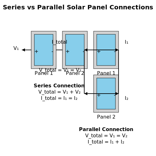
When connecting solar panels in series, the voltages add while the current remains constant. For n identical panels with open-circuit voltage VOC and short-circuit current ISC, the total output becomes:
In parallel configurations, currents add while voltage stays fixed:
Power Output and MPPT Implications
Maximum Power Point Tracking (MPPT) algorithms must account for configuration differences. Series connections increase voltage, reducing resistive losses in long wire runs but require higher-voltage-rated components. Parallel configurations minimize voltage drop mismatches but need robust current-handling capacity.
where η represents system efficiency losses from wiring, diodes, or shading.
Shading and Fault Tolerance
Series strings suffer significant power loss under partial shading due to current bottlenecks. Bypass diodes mitigate this by creating alternative current paths. Parallel configurations inherently tolerate shading better but require blocking diodes to prevent reverse currents.
Practical Design Considerations
- Series advantages: Lower wire gauges, simpler MPPT optimization, reduced combiner box complexity
- Parallel advantages: Better shade tolerance, modular maintenance, safer low-voltage operation
- Hybrid systems: Series-parallel combinations balance voltage/current requirements (e.g., 2S2P for 24V systems)
Mathematical Optimization Example
For a system requiring 48V with four 12V/5A panels, compare configurations:
Wire losses Ploss favor higher-voltage configurations:
2.3 Charge Controllers: PWM vs. MPPT
Fundamental Operating Principles
The primary function of a charge controller in a solar panel system is to regulate the voltage and current from the photovoltaic (PV) array to the battery bank, ensuring optimal charging while preventing overcharge or deep discharge. Two dominant technologies exist: Pulse-Width Modulation (PWM) and Maximum Power Point Tracking (MPPT). Their operational differences stem from their underlying control mechanisms.
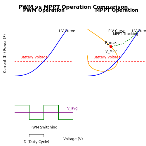
A PWM controller operates as a switch between the solar array and the battery, connecting and disconnecting at high frequency to maintain the battery at the desired voltage. The duty cycle of the PWM signal adjusts based on the battery's state of charge. Mathematically, the average voltage delivered to the battery is:
where D is the duty cycle (0 ≤ D ≤ 1) and VPV is the solar panel's output voltage. Since the panel voltage is pulled down to the battery voltage, PWM controllers are most efficient when VPV is close to the battery voltage.
MPPT: Dynamic Power Optimization
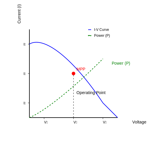
An MPPT controller actively tracks the maximum power point (MPP) of the solar array, where the product of current and voltage is maximized. The MPP varies with irradiance and temperature, described by the PV cell's current-voltage (I-V) and power-voltage (P-V) characteristics. The controller continuously adjusts the operating point using a DC-DC converter (typically buck or buck-boost) to extract maximum available power.
The power optimization process involves solving:
where P = VI. For a solar cell, the current I is given by the single-diode model:
Here, Iph is the photocurrent, I0 the reverse saturation current, Rs and Rsh the series and shunt resistances, and n the ideality factor. MPPT algorithms (e.g., Perturb and Observe, Incremental Conductance) iteratively solve this to locate the MPP.
Efficiency Comparison
MPPT controllers typically achieve 93–97% efficiency, while PWM controllers range from 65–80%. The key advantage of MPPT arises in scenarios where VPV significantly exceeds the battery voltage (e.g., cold climates or partial shading). The power gain is quantified as:
For example, a 36V panel charging a 12V battery through a PWM controller wastes up to 66% of available power, whereas an MPPT controller converts the excess voltage into additional current.
Practical Considerations
- Cost: MPPT controllers are 2–3× more expensive than PWM but justify the cost in systems >200W or with high VPV–Vbatt mismatch.
- Scalability: MPPT supports higher voltage arrays (up to 600V), reducing wiring losses.
- Temperature Effects: PWM efficiency drops sharply in low temperatures due to increased VMPP.
Real-World Applications
In grid-tied systems, MPPT is ubiquitous due to its voltage flexibility and compliance with inverter requirements. Off-grid applications (e.g., remote telecom) favor MPPT for its tolerance to partial shading and battery voltage fluctuations. PWM remains viable for small-scale systems (e.g., RVs, marine) where cost and simplicity outweigh efficiency losses.
3. Selecting the Right Battery for Solar Applications
3.1 Selecting the Right Battery for Solar Applications
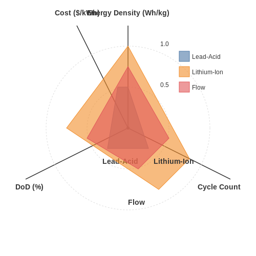
The choice of battery in a solar energy system critically impacts efficiency, longevity, and cost. Key parameters include energy density, cycle life, depth of discharge (DoD), and charge/discharge efficiency. Lead-acid, lithium-ion, and flow batteries dominate the market, each with distinct trade-offs.
Battery Chemistry Comparison
Lead-acid batteries remain prevalent due to low upfront cost, but suffer from limited cycle life (300–500 cycles at 50% DoD) and low energy density (30–50 Wh/kg). Lithium-ion batteries, particularly LiFePO4, offer superior cycle life (2000–5000 cycles at 80% DoD) and energy density (90–160 Wh/kg), albeit at higher cost. Flow batteries (e.g., vanadium redox) excel in scalability and longevity (10,000+ cycles) but have low energy density (20–50 Wh/kg).
Mathematical Modeling of Battery Performance
The usable capacity Cusable of a battery depends on its depth of discharge:
where Crated is the manufacturer's rated capacity. The total energy throughput Etotal over the battery's lifetime is:
Here, Ncycles is the cycle life at the chosen DoD, and η is the round-trip efficiency (typically 70–95%).
Temperature Effects and Derating
Battery capacity degrades at extreme temperatures. The Arrhenius equation models temperature-dependent capacity loss:
where k is the degradation rate, Ea is activation energy (chemistry-dependent), and T is temperature in Kelvin. Lead-acid batteries lose ~1% capacity per °C below 25°C, while lithium-ion degrades faster above 45°C.
Case Study: Off-Grid System Sizing
For a 5 kW solar array with 20 kWh daily load, compare lithium-ion vs. lead-acid:
- Lithium-ion: 24 kWh bank (80% DoD) lasts 10+ years
- Lead-acid: 40 kWh bank (50% DoD) requires replacement every 3–5 years
The levelized cost of storage (LCOS) favors lithium-ion for systems with >1500 equivalent full cycles.
Emerging Technologies
Solid-state lithium batteries promise energy densities >400 Wh/kg with improved safety. Sodium-ion batteries offer cost advantages for stationary storage, with recent prototypes achieving 160 Wh/kg and 3000+ cycles.
3.2 Battery Charging and Discharging Cycles
Charge-Discharge Fundamentals
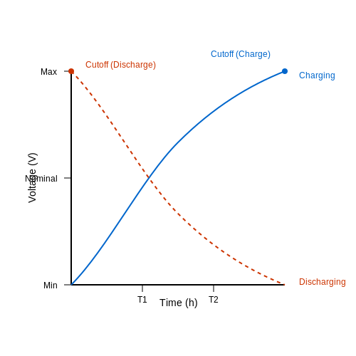
The electrochemical dynamics of a battery during charging and discharging are governed by redox reactions at the electrodes. During discharging, the anode undergoes oxidation (releasing electrons), while the cathode experiences reduction (consuming electrons). The reverse occurs during charging, where an external voltage source drives electrons back to the anode.
The total charge capacity Q of a battery is defined as:
where I is the discharge current and t is the time until the cutoff voltage is reached. For lithium-ion batteries, this is typically 2.5–3.0V per cell.
Depth of Discharge (DoD) and Cycle Life
The relationship between Depth of Discharge (DoD) and cycle life follows a logarithmic decay:
where N is the cycle count at a given DoD, N0 is the cycle count at 100% DoD, and α is the battery-specific degradation coefficient. For example, a LiFePO4 battery cycled at 20% DoD may achieve 7,000 cycles, while 80% DoD reduces this to 2,000 cycles.
Charge Control Algorithms
Modern solar charge controllers implement multi-stage charging:
- Bulk Charge: Constant current (CC) until ~80% State of Charge (SoC)
- Absorption: Constant voltage (CV) until current drops below C/20
- Float: Reduced voltage to compensate for self-discharge
The transition points are temperature-compensated using the Nernst equation:
Peukert's Law for Capacity Adjustment
At high discharge rates, apparent capacity decreases due to Peukert's effect:
where Cp is the Peukert capacity, I is the discharge current, t is time, and k is the Peukert exponent (typically 1.05–1.15 for Li-ion, 1.2–1.6 for lead-acid).
State of Health (SoH) Estimation
SoH is calculated through impedance spectroscopy and coulomb counting:
Advanced BMS systems track incremental capacity analysis (ICA) by differentiating charge curves:
Peak shifts in dQ/dV plots indicate degradation mechanisms like lithium plating or SEI growth.
3.3 Overcharge and Deep Discharge Protection
In solar panel circuits, battery longevity critically depends on preventing overcharge and deep discharge. Both conditions degrade battery chemistry, reducing capacity and cycle life. Advanced charge controllers employ voltage thresholds, hysteresis control, and adaptive algorithms to mitigate these risks.
Voltage Thresholds and Hysteresis Control
Overcharge protection is typically implemented by monitoring the battery voltage (Vbat) and disconnecting the solar input when Vbat exceeds a predefined upper limit (Voc). For a 12V lead-acid battery, Voc ≈ 14.4V (at 25°C). The controller reconnects the solar input once Vbat drops below a hysteresis threshold (Vreconnect ≈ 13.2V). This prevents rapid cycling near the cutoff voltage.
where Vnom is the nominal float voltage, ΔVtemp compensates for temperature variations (typically −3 mV/°C/cell for lead-acid), and ΔVaging accounts for increased internal resistance over time.
State of Charge (SoC) Estimation
Deep discharge protection requires accurate SoC estimation. Coulomb counting integrates current over time, but errors accumulate due to self-discharge and inefficiencies. Advanced systems combine coulomb counting with open-circuit voltage (OCV) measurements during idle periods:
where Qn is the nominal capacity, I is the discharge current, and η is the self-discharge rate. Kalman filters or neural networks further refine SoC estimates in modern BMS designs.
Active Balancing vs. Dissipative Methods
Lithium-ion batteries require cell-level balancing to prevent overcharge of individual cells. Dissipative balancing bleeds excess energy through resistors, while active balancing redistributes charge using switched capacitors or inductors. The power loss (Pdiss) for resistive balancing is:
where Vi is the cell voltage, Ri is the balancing resistor, and N is the number of cells. Active balancing achieves higher efficiency but increases circuit complexity.
Case Study: Maximum Power Point Tracking (MPPT) Controllers
MPPT controllers dynamically adjust the solar array’s operating point to avoid overcharging while maximizing harvest. A perturb-and-observe algorithm compares dP/dV to track the peak power voltage (Vmpp):
When dP/dV > 0, the controller increases V; when dP/dV < 0, it decreases V. This ensures the battery charges at the optimal rate without exceeding Voc.
4. Understanding DC to AC Conversion
4.1 Understanding DC to AC Conversion
Fundamentals of Power Inversion
The conversion of DC to AC power requires active switching elements to reconstruct an alternating waveform from a direct current source. Unlike passive rectification, inversion is fundamentally a nonlinear process that synthesizes an AC waveform through pulse-width modulation (PWM) or multilevel switching techniques. The quality of inversion depends on three key parameters: total harmonic distortion (THD), switching frequency, and output impedance.
Topologies for Solar Applications
Modern solar inverters primarily use one of three architectures:
- H-bridge converters - Four switching elements creating bipolar output
- Three-phase voltage source inverters - For industrial-scale systems
- Z-source inverters - Provide voltage boost capability in a single stage
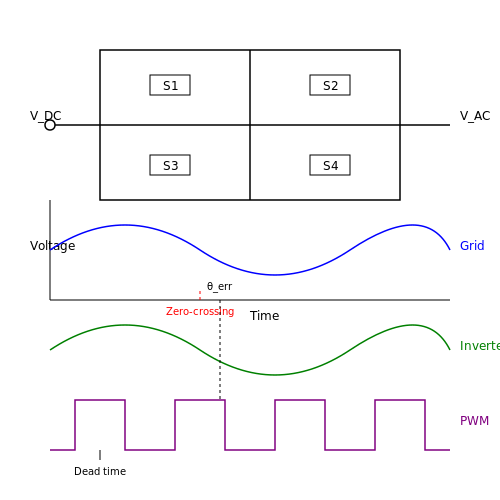
The H-bridge configuration dominates residential applications due to its simplicity and ability to generate pure sine waves when combined with proper filtering. The switching sequence follows:
Maximum Power Point Tracking Integration
Effective DC-AC conversion in solar systems requires dynamic impedance matching through MPPT algorithms. The perturbation and observation method continuously adjusts the inverter's input resistance to maintain operation at the PV array's peak power voltage:
Modern inverters implement this through predictive current control loops that sample array voltage and current at frequencies exceeding 10 kHz.
Grid-Tie Synchronization
For utility-connected systems, the inverter must phase-lock to the grid using a phase-locked loop (PLL) circuit. The synchronization error must be maintained within 0.5° for IEEE 1547 compliance. The PLL compares zero-crossings of the inverter output with the grid waveform, adjusting the PWM timing to minimize phase error:
Efficiency Considerations
State-of-the-art solar inverters achieve 97-99% peak efficiency through:
- Silicon carbide (SiC) MOSFETs with RDS(on) < 15mΩ
- Interleaved boost converters reducing input current ripple
- Advanced thermal management keeping junction temperatures below 125°C
The European efficiency metric (ηEU) weights performance across multiple operating points:
4.2 Pure Sine Wave vs. Modified Sine Wave Inverters
Fundamental Waveform Characteristics
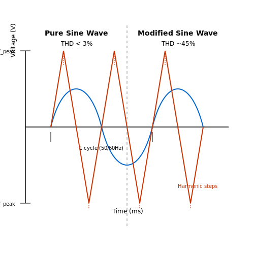
The primary distinction between pure sine wave (PSW) and modified sine wave (MSW) inverters lies in their output voltage waveforms. A pure sine wave inverter generates a smooth, continuous sinusoidal voltage defined by:
where Vpeak is the peak voltage and f is the fundamental frequency (typically 50Hz or 60Hz). In contrast, a modified sine wave approximates this using a stepped waveform composed of discrete voltage levels, often implemented through pulse-width modulation (PWM) techniques.
Harmonic Distortion and Power Quality
PSW inverters exhibit total harmonic distortion (THD) below 3%, making them ideal for sensitive electronics. The THD for an MSW inverter can exceed 40%, introducing significant higher-order harmonics:
where Vh represents the RMS voltage of the h-th harmonic component. These harmonics cause:
- Increased heating in inductive loads (motors, transformers)
- Audible noise in audio equipment
- Interference with communication devices
Efficiency and Switching Losses
While MSW inverters achieve 85-90% efficiency due to simpler switching topologies, PSW inverters using multilevel or H-bridge configurations reach 92-96% efficiency through advanced control algorithms. The power dissipation in switching devices follows:
where tr and tf are the rise/fall times, and fsw is the switching frequency.
Applications and Load Compatibility
PSW inverters are mandatory for:
- Medical imaging equipment (MRI, CT scanners)
- Variable frequency drives
- Precision laboratory instruments
MSW inverters suffice for resistive loads like incandescent lighting or simple heating elements, where waveform fidelity is less critical.
Design Tradeoffs and Cost Analysis
The bill of materials (BOM) difference stems from:
| Component | PSW | MSW |
|---|---|---|
| Control IC | DSP-based (e.g., TI C2000) | Basic PWM controller |
| Filtering | LC network (Q>50) | Minimal capacitance |
| Switches | SiC/GaN FETs | IGBT modules |
This results in a 2-3x cost premium for PSW inverters above 1kW ratings.
4.3 Grid-Tied vs. Off-Grid Inverter Systems
Fundamental Operational Differences
Grid-tied and off-grid inverter systems differ primarily in their interaction with the utility grid. A grid-tied inverter synchronizes its output voltage, frequency, and phase with the grid, enabling bidirectional power flow. The inverter must adhere to IEEE 1547 and UL 1741 standards for anti-islanding protection. In contrast, an off-grid inverter operates independently, supplying power directly to local loads without synchronization requirements. Its voltage and frequency regulation rely solely on internal control loops.
Power Flow and Energy Management
The power flow equation for a grid-tied system is given by:
where Pgrid is the power drawn from (positive) or fed into (negative) the grid, Pload is the load demand, and PPV is the photovoltaic generation. Off-grid systems must balance generation and demand instantaneously, often requiring battery storage:
where Ebat is the battery energy and Ploss accounts for conversion losses.
Control Architectures
Grid-tied inverters typically employ dq-current control in the synchronous reference frame:
where vd, vq are inverter voltages, id, iq are currents, L is filter inductance, and ω is grid angular frequency. Off-grid inverters use voltage-mode control with droop characteristics to maintain stability under varying loads:
Efficiency and Cost Considerations
Grid-tied systems achieve higher efficiency (typically 97-98%) by eliminating battery conversion losses. However, they require expensive grid compliance certifications. Off-grid systems have lower round-trip efficiency (85-92%) due to battery losses but provide energy independence. The levelized cost of energy (LCOE) for off-grid systems is given by:
where Ccap is capital cost, CO&M,t is operation/maintenance cost at time t, Egen,t is energy generated, and r is discount rate.
Real-World Implementation Challenges
Grid-tied systems face challenges with harmonic injection (THD < 5% per IEEE 519) and reactive power compensation. Off-grid systems must handle load transients and state-of-charge management. Modern solutions employ model predictive control (MPC) for grid-tied systems and adaptive droop control for off-grid microgrids.
5. Performance Monitoring Systems
5.1 Performance Monitoring Systems
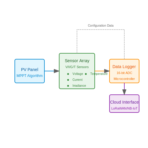
Performance monitoring in solar panel circuits is critical for ensuring optimal energy harvest, fault detection, and long-term reliability. Advanced monitoring systems integrate real-time data acquisition, power analytics, and predictive maintenance algorithms.
Key Parameters and Measurement Techniques
The primary electrical parameters monitored include:
- Voltage (V) — Measured across the panel or string using high-impedance differential amplifiers to minimize loading effects.
- Current (I) — Captured via shunt resistors, Hall-effect sensors, or Rogowski coils, with trade-offs in accuracy and bandwidth.
- Irradiance (G) — Quantified using calibrated reference cells or pyranometers, often normalized to Standard Test Conditions (STC).
- Temperature (T) — Tracked with PT100 or thermocouple sensors, critical for derating power output.
Mathematical Modeling of Performance Metrics
The instantaneous power output of a solar panel is given by:
For maximum power point tracking (MPPT), the fill factor (FF) is derived as:
where Voc is the open-circuit voltage and Isc is the short-circuit current. The panel's efficiency (η) under real-world conditions is:
where A is the panel area. Temperature effects are modeled using the empirical relation:
where βV is the temperature coefficient of voltage (typically -0.3%/°C for silicon cells).
Data Acquisition and Telemetry
Modern monitoring systems employ:
- High-resolution ADCs (16-bit or higher) for precise analog-to-digital conversion.
- Time-synchronized sampling to align voltage/current measurements and compute true power.
- Wireless protocols like LoRaWAN or NB-IoT for remote installations, with packet loss mitigation through redundant transmission.
Fault Detection Algorithms
Common diagnostic methods include:
- Current-voltage (I-V) curve analysis — Detects partial shading, PID (potential-induced degradation), or cell cracks by comparing measured curves to theoretical models.
- Statistical outlier detection — Uses machine learning (e.g., k-nearest neighbors) to identify underperforming panels in large arrays.
- Impedance spectroscopy — Measures frequency-dependent impedance to diagnose aging or moisture ingress.
Case Study: Distributed Monitoring in Utility-Scale PV Plants
A 100 MW solar farm in Arizona implemented module-level monitoring with:
- DC optimizers at each panel (0.1% current measurement accuracy).
- Mesh networking for data aggregation.
- Cloud-based analytics reducing O&M costs by 18% through predictive fault detection.
5.2 Troubleshooting Common Issues
Open-Circuit Voltage (VOC) Anomalies
An unexpected drop in VOC often indicates cell degradation or partial shading. The theoretical VOC of a solar cell is given by:
where n is the ideality factor, kB is Boltzmann's constant, T is temperature, q is electron charge, IL is light-generated current, and I0 is reverse saturation current. A 10% deviation from the expected VOC suggests potential bypass diode failure or PID (Potential Induced Degradation).
Hot Spots and Reverse Bias Effects
When a cell underperforms (due to shading or damage), it operates in reverse bias, dissipating power as heat. The power dissipation Pdiss in a shaded cell can be modeled as:
where IMPP and VMPP are current and voltage at maximum power point. Bypass diodes with a forward voltage drop VF < 0.7V should be tested using an IV curve tracer.
Microcracks and Cell Fractures
Electroluminescence imaging reveals microcracks invisible to the naked eye. The fracture resistance Rf of silicon cells follows:
where KIC is fracture toughness (0.75 MPa√m for monocrystalline Si) and a is crack length. Cracks >3mm typically cause >5% power loss due to interrupted current pathways.
PID and Leakage Currents
Potential Induced Degradation manifests as increased leakage current Ileak through the panel's insulation:
where Yinsulation is admittance and Cinsulation is capacitance. PID testing requires applying ±1000V DC between cell and frame while monitoring insulation resistance (should be >40MΩ).
Mismatch Losses in Arrays
Current mismatch between parallel strings causes efficiency loss ηloss:
For <5% loss, ensure ΔVMPP < 3% and ΔISC < 1% across all panels. Infrared thermography helps identify mismatched modules operating at different temperatures.
Inverter Synchronization Issues
Grid-tied inverters must maintain phase lock with utility voltage Vgrid. The phase error θerr affects power injection:
where X is line reactance. A PLL (Phase-Locked Loop) with <0.5° jitter is critical for stable operation. Oscilloscope measurements should show THD <3% and frequency drift <0.1Hz.
5.3 Preventive Maintenance Practices
Thermal Monitoring and Mitigation
Solar panels experience thermal cycling due to diurnal temperature variations, which can induce mechanical stress in photovoltaic (PV) cells and interconnects. The thermal coefficient of power (β) for silicon-based cells is typically -0.4% to -0.5%/°C, meaning efficiency drops as temperature rises. To mitigate this:
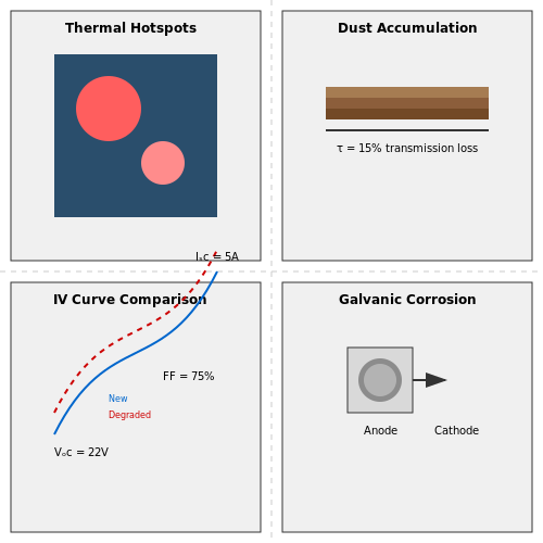
where PSTC is power at Standard Test Conditions (25°C), and Tactual is the module's operating temperature. Infrared thermography should be performed quarterly to identify hotspots caused by:
- Partial shading (bypass diode failure)
- Microcracks (cell fractures)
- Degraded solder bonds
Soiling and Environmental Contamination
Dust accumulation follows a non-linear transmission loss model:
where α is the attenuation coefficient (m-1), d is dust thickness, and AF is the angular correction factor for incident light. For arid climates, monthly cleaning with deionized water (resistivity >18 MΩ·cm) prevents:
- Mineral deposition (calcite, gypsum)
- Pollen adhesion
- Bird droppings (pH-driven corrosion)
Electrical Parameter Drift Analysis
Use IV curve tracers to track deviations from baseline parameters:
| Parameter | Acceptable Drift | Failure Threshold |
|---|---|---|
| VOC | ±3% | ±10% |
| ISC | ±5% | ±15% |
| FF | ±5% | ±20% |
Electroluminescence imaging should be conducted annually to detect:
- Potential-induced degradation (PID)
- Light-induced degradation (LID)
- Contact delamination
Mechanical Integrity Checks
Modal analysis of mounting structures should verify natural frequencies (fn) avoid wind-induced resonance:
where k is structural stiffness (N/m) and m is mass (kg). Torque audits on rail fasteners must maintain:
- 20-25 N·m for aluminum rails
- 30-35 N·m for steel rails
Corrosion Prevention
Galvanic corrosion at dissimilar metal junctions follows Faraday's law:
where m is mass loss, I is current, t is time, M is molar mass, n is valence electrons, and F is Faraday's constant. Apply:
- Zinc-rich primers for coastal installations
- Dielectric grease on terminal blocks
- Anodized aluminum for frame grounding
6. Maximum Power Point Tracking (MPPT) Algorithms
6.1 Maximum Power Point Tracking (MPPT) Algorithms
Photovoltaic (PV) systems exhibit a nonlinear current-voltage (I-V) characteristic, where the power output varies with irradiance, temperature, and load conditions. The Maximum Power Point (MPP) represents the optimal operating point where the product of voltage and current maximizes power extraction. MPPT algorithms dynamically adjust the load impedance to maintain operation at this point despite environmental fluctuations.
Fundamentals of MPPT Operation
The power-voltage (P-V) curve of a solar panel demonstrates a single global maximum under uniform irradiance, though partial shading may introduce local maxima. The MPP satisfies the condition:
where P is panel power and V is output voltage. This translates to the impedance matching requirement:
where Rpanel is the panel's equivalent resistance at MPP. DC-DC converters implement this impedance transformation through duty cycle control.
Perturb and Observe (P&O) Algorithm
The most widely implemented MPPT method uses hill-climbing principles:
- Measure current panel voltage V(k) and current I(k)
- Calculate power P(k) = V(k) × I(k)
- Compare with previous power P(k-1)
- Adjust voltage reference Vref in the perturbation direction if ΔP > 0
- Reverse direction if ΔP < 0
The algorithm's effectiveness depends on perturbation step size - larger steps improve tracking speed but increase steady-state oscillation. Advanced implementations use adaptive step sizing:
where K is a convergence constant. Field tests show P&O achieves 97-99% efficiency under stable irradiance but suffers from drift during rapidly changing conditions.
Incremental Conductance Method
This technique eliminates P&O's steady-state oscillation by directly solving the MPP condition:
The implementation compares instantaneous conductance (I/V) with incremental conductance (ΔI/ΔV):
| Condition | MPP Position | Action |
|---|---|---|
| ΔI/ΔV = -I/V | At MPP | Maintain Vref |
| ΔI/ΔV > -I/V | Left of MPP | Increase Vref |
| ΔI/ΔV < -I/V | Right of MPP | Decrease Vref |
This method achieves 99.5% efficiency in laboratory conditions but requires high-precision current sensors and faster sampling than P&O.
Model-Based Techniques
Advanced MPPT implementations incorporate PV modeling to predict the MPP location:
Fractional Open-Circuit Voltage
Exploits the near-linear relationship between VMPP and open-circuit voltage VOC:
where k (typically 0.70-0.78) is determined empirically. The system periodically measures VOC during brief load disconnections.
Neural Network MPPT
Multilayer perceptrons trained on historical I-V curves can estimate MPP voltage with <1% error. Input features typically include:
- Irradiance estimates from photodiodes
- Panel temperature measurements
- Historical operating points
Field deployments show 2-3% better energy harvest than conventional algorithms under partial shading, at the cost of increased computational requirements.
Global Peak Tracking Under Partial Shading
When bypass diodes activate due to cell mismatch, the P-V curve develops multiple local maxima. Modern solutions include:
- Sweep scanning: Temporarily varies voltage across the full operating range to identify the global peak
- Particle swarm optimization: Uses parallel search agents to explore the solution space
- Impedance matching networks: Dedicated converters for submodule-level MPPT
Experimental results demonstrate 12-25% energy recovery compared to conventional MPPT in heavy shading scenarios.
6.2 Solar Tracking Systems for Enhanced Efficiency
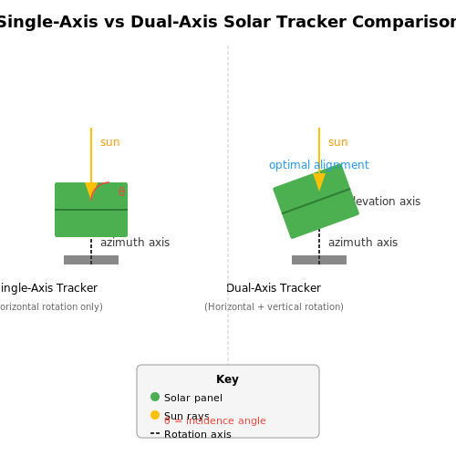
Solar tracking systems dynamically adjust the orientation of photovoltaic (PV) panels to maintain optimal alignment with the sun, maximizing energy capture. Unlike fixed-tilt systems, which suffer from cosine losses due to misalignment, tracking systems minimize the angle of incidence (θ) between incoming sunlight and the panel surface. The power output of a solar panel is governed by:
where I0 is the solar irradiance, A is the panel area, and θ is the incidence angle. A dual-axis tracker eliminates cosine losses entirely at solar noon, while single-axis trackers reduce but do not eliminate them.
Types of Solar Tracking Systems
Single-axis trackers rotate along one axis (typically north-south), following the sun’s east-west movement. The power gain over a fixed system is approximated by:
Dual-axis trackers adjust both azimuth and elevation, maintaining near-perpendicular alignment. Their efficiency is derived from the solid angle integral:
Control Strategies
Tracking systems employ either:
- Closed-loop control: Light-dependent resistors (LDRs) or photodiodes provide real-time feedback to a PID controller, minimizing error between panel and sun position.
- Open-loop control: Astronomical algorithms compute sun position based on latitude, longitude, and time, driving stepper or servo motors.
The error dynamics of a PID-controlled tracker are modeled as:
where τ is the motor time constant, ζ is damping, and Kp is the proportional gain.
Mechanical Design Considerations
Torque requirements for a panel of mass m and length L are calculated from:
High-precision helical gearboxes (e.g., 100:1 reduction) are often paired with NEMA 17 stepper motors (holding torque ≥ 40 N·cm) to overcome wind loads up to 25 m/s.
Energy Yield vs. Cost Tradeoffs
Dual-axis systems increase energy yield by 30–45% over fixed systems but require 2–3× higher capital expenditure. The net present value (NPV) of a tracker is evaluated using:
where ΔPt is the additional energy produced, Celec is electricity cost, and r is the discount rate. Commercial systems typically achieve payback periods of 5–8 years.
6.3 Integration with Smart Grids and IoT
Smart Grid Architecture and Solar Integration
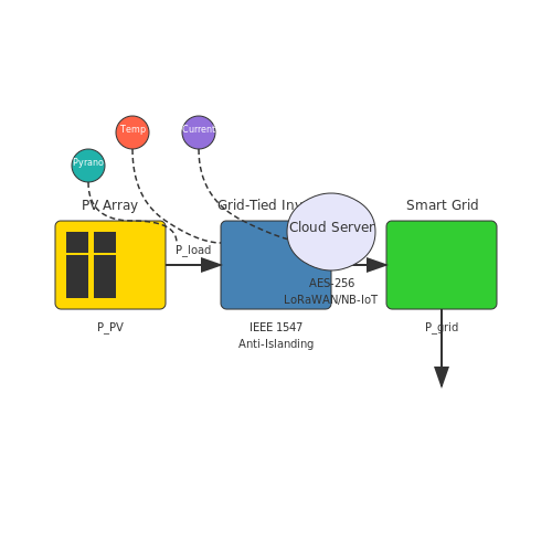
Modern smart grids incorporate bidirectional power flow, real-time monitoring, and demand-response mechanisms. Solar panel circuits interface with smart grids through grid-tied inverters, which synchronize photovoltaic (PV) output with grid voltage and frequency. The inverter's role extends beyond DC-AC conversion—it must also implement anti-islanding protection to disconnect during grid outages, as per IEEE 1547 standards.
The power flow equation for a grid-connected solar system is:
where Pgrid is the net power exchanged with the grid, PPV is the solar generation, Pload is local consumption, and Ploss accounts for conversion and transmission losses.
IoT-Enabled Solar Monitoring
Internet of Things (IoT) devices enhance solar circuit performance through distributed sensor networks. Key parameters monitored include:
- Irradiance (via pyranometers or reference cell measurements)
- Module temperature (PT100 or thermistor-based)
- String currents (Hall-effect sensors)
- Bus voltages (isolated differential amplifiers)
An IoT node typically transmits data through LoRaWAN or NB-IoT protocols, with sampling intervals optimized using Nyquist criteria for the system's dominant time constants. The maximum sampling period for a solar array with 10 ms transient response is:
Dynamic Load Balancing with Machine Learning
Advanced smart grids employ machine learning (ML) to predict solar generation and optimize load distribution. A recurrent neural network (RNN) trained on historical weather and generation data can forecast PV output with mean absolute errors below 5%. The prediction model minimizes the cost function:
where hθ(x) is the hypothesis function, λ is the regularization parameter, and m is the training set size.
Case Study: Virtual Power Plants (VPPs)
In Berlin's enera project, 1,200 residential PV systems aggregate into a VPP using blockchain for decentralized coordination. Each 5 kW system contributes to grid stability by adjusting reactive power (Q) according to:
where S is the apparent power limit of the inverter. The VPP reduces grid congestion by 18% compared to standalone solar systems.
Cybersecurity Considerations
Solar-integrated smart grids require robust encryption for IoT communications. AES-256 encryption is standard for meter data, while blockchain secures peer-to-peer energy trading. Man-in-the-middle attacks are mitigated through:
- DTLS handshakes for LoRaWAN
- Hardware security modules (HSMs) in inverters
- Quantum-resistant lattice-based cryptography in next-gen systems
7. Essential Books on Solar Panel Circuits
7.1 Essential Books on Solar Panel Circuits
- Design and implementation of a waterless solar panel cleaning system — Manual cleaning of large solar installations is often labor-intensive and time-consuming, primarily due to the accumulation of dust on solar panels, which significantly impairs their efficiency. The study introduces a novel, waterless, cost-effective automatic cleaning system for small solar panels.
- PDF Solar & Wind Electrical Systems - MRCET — The basic concepts of solar energy, solar radiation and fundamentals of wind turbines. Different types of Solar cells, Solar power systems and their integration. Generation schemes with both constant & variable speed turbines and different types of Generat Various other subsystems of Solar and Wind based power plants and their Integration with ...
- PDF 500 Electronic Projects For Inventors With Tested Circuits — 500 Electronic Projects for Inventors: Tested Circuits and Inspiring Ideas Embarking on a journey into the world of electronics can be daunting. Where do you start? This article introduces a treasure trove of 500 electronic projects designed for inventors at all skill levels, featuring tested circuits and clear explanations.
- Solar PV systems design and monitoring - ScienceDirect — A solar photovoltaic (PV) system includes the main components of PV modules, a solar inverter, and a bias of system (BoS), which can generate AC and DC power. However, the desired efficiency of PV systems relies on many factors as well as understanding the component functionality and configuration. Moreover, comprehension of the monitoring techniques and reliable engineering methods are ...
- Photovoltaic system - Wikipedia — A photovoltaic system, also called a PV system or solar power system, is an electric power system designed to supply usable solar power by means of photovoltaics. It consists of an arrangement of several components, including solar panels to absorb and convert sunlight into electricity, a solar inverter to convert the output from direct to alternating current, as well as mounting, cabling, and ...
- MPPT methods for solar PV systems: a critical review based on tracking ... — The rest of the paper is organised as follows. In Section 2, a model of the solar PV system with its characteristics, equivalent circuit, effect of temperature, insolation, and PSC on maximum power are presented. The need for the MPPT controller, its selection parameters, and PSC supported MPPT methods are described in Section 3.
- Power Electronic Converters for Solar Photovoltaic Systems — Solar power has a lower environmental impact than other renewable energy sources. DC-DC converters are utilized to obtain the necessary voltage level from the photovoltaic (PV) system.
- Critical review on various inverter topologies for PV system ... — The dynamic nature of solar insolation directly results in the power output of the PV. So, in single-stage grid-connected PV systems, the primary task of the inverter is to track MPP in any irradiation and configuration model.
- Altitude's Impact on Photovoltaic Efficiency: An IoT-Enabled ... — For the measurement of the efficiency of the PV panels, an electronic circuit was developed to obtain fast and high-precision I-V curves in real-time. We have developed a user-friendly web platform that serves as a single-entry point for remotely controlling our network of PV systems distributed across various geographical locations and altitudes.
- (PDF) Stand-Alone Photovoltaic System - ResearchGate — In book: Energy Science and Technology Vol. 6: Solar Engineering (pp.141 - 163) Chapter: 5 Stand-Alone Photovoltaic System Publisher: Studium Press LLC Editors: N.J. Govil
7.2 Research Papers and Journals
- Thermal Management of Solar Panels for Overall Efficiency Enhancement ... — Solar energy offers various advantages, including ease of access and improved predictability compared to other renewable energy sources in vogue. This energy source is used for a variety of applications, including power generation, desalination, and heating. PV panels are commonly used to generate direct electricity. The acquired solar thermal energy, on the other hand, it can be used to ...
- PDF International Journal of Research Publication and Reviews Solar ... — Overall, this project combines hardware design, software programming, and control algorithms to create an intelligent solar tracking system that optimizes the positioning of solar panels for enhanced energy harvesting
- PDF A study of solar photovoltaic systems and its applications in modern ... — However, this technique requires periodical short-circuit of the PV panel to measure the relevant current as a reference which will result in more power loss, and damages may happen for the electrical and electronic devices [99,100].
- Electronic Control Circuit for Solar Battery Charging — An electronic circuit is designed, built and tested. The circuit acts as a control circuit to regulate the process of photovoltaic solar panel battery charging process.
- A Review of Time-Based Solar Photovoltaic Tracking Systems — This paper aims to bridge these gaps by extensively reviewing these time-based solar tracking systems based on axis rotation and drive types. Lessons learned from the comprehensive review have been highlighted and discussed. Finally, critical open research issues are identified and elaborated.
- Up-to-date literature review on Solar PV systems: Technology progress ... — This review presents updated information on the solar PV development from the material, market, and engineering perspectives. Cell efficiencies, market trends, cost of PV systems, and global research efforts over the last years are provided. Real monitored performances reveal a decrease of up to 10% of PV power output due to soiling effects.
- Design and Analysis of a Solar-Powered Electric Vehicle Charging ... — This paper presents results from the design of a solar-powered EV charging station for an Indian context. PVsyst 7.2 software has been used for the system design.
- MPPT methods for solar PV systems: a critical review based on tracking ... — The rest of the paper is organised as follows. In Section 2, a model of the solar PV system with its characteristics, equivalent circuit, effect of temperature, insolation, and PSC on maximum power are presented. The need for the MPPT controller, its selection parameters, and PSC supported MPPT methods are described in Section 3.
- A Review of Multilevel Inverter Topologies for Grid-Connected ... — Solar energy is one of the most suggested sustainable energy sources due to its availability in nature, developments in power electronics, and global environmental concerns. A solar photovoltaic system is one example of a grid-connected application using multilevel inverters (MLIs). In grid-connected PV systems, the inverter's design must be carefully considered to improve efficiency. The ...
- Critical review on various inverter topologies for PV system ... — This paper has presented a detailed review of different PV inverter topologies for PV system architectures and concluded as: except if high voltage is available at input single-stage centralised inverters should be side-stepped, to avoid further voltage amplification.
7.3 Online Resources and Tutorials
- PDF Power Electronics Handbook Third Edition - aram.xkcd.com — Power Electronics Handbook Fraidoon MAZDA,1997 Written by a practising electronics engineer for practising engineers this reference covers the design of power circuits This edition has been updated and expanded to include a new chapter on Smart Power power integrated circuits SPICE for Power Electronics and Electric Power Muhammad H. Rashid ...
- PDF 500 Electronic Projects For Inventors With Tested Circuits — Imagine having access to a library of tested electronic projects, meticulously documented and ready for adaptation and improvement. This is the promise of a collection like "500 Electronic Projects for Inventors with Tested Circuits." But what exactly does this offer, and how can inventors utilize such a resource?
- Solar panel - Wikipedia — Greencap Energy solar array mounted on brewery in Worthing, England Solar array mounted on a rooftop A solar panel is a device that converts sunlight into electricity by using photovoltaic (PV) cells. PV cells are made of materials that produce excited electrons when exposed to light. These electrons flow through a circuit and produce direct current (DC) electricity, which can be used to power ...
- Solar Fan Aspirated WiFi Weather Station - Hackster.io — Electronics Enclosure Outdoor circuits should be protected from moisture, sunlight, and temperature extremes. However, there obviously are components which need to be exposed to a certain degree: the solar panel, ventilation fan, and the environmental sensor.
- Design and Performance Analysis of Foldable Solar Panel for ... — This study investigates the use of a foldable solar panel system equipped with a dynamic tracking algorithm for agrivoltaics system (AVS) applications. It aims to simultaneously meet the requirements for renewable energy and sustainable agriculture. The design focuses on improving solar energy capture while facilitating crop growth through adjustable shading. The results show that foldable ...
- Stepâ byâ Step Design of Largeâ Scale ... - Wiley Online Library — Chapter 5 conducts a compre-hensive discussion on radiometric terms, arrangement of solar resources, and main parameters of solar energy radiation. A detailed review on engineering doc-uments and their classification for LS-PVPP projects is presented in Chapter 6.
- Wiki Complete Electronics Tutorial - The Powder Toy — This page is currently a work in progress. The goal of this page is to be a complete electronics tutorial for new players and seasoned ones who want to learn more about electronics, and to replace the existing electronics tutorial that has not been updated since 2011.
- Module Circuit Design - PVEducation — An individual silicon solar cell has a voltage at the maximum power point around 0.5V under 25 °C and AM1.5 illumination. Taking into account an expected reduction in PV module voltage due to temperature and the fact that a battery may require voltages of 15V or more to charge, most modules contain 36 solar cells in series.
- Capstone_Project/001_Amazon_Electronics_Capstone.ipynb at main ... — Light, Heat, Sound, and Electricity', 'Electronics for Kids: Play with Simple Circuits and Experiment with Electricity!', 'Minecraft Kids Smart Watch - Touchscreen Interactive Watch with 10 Customizable Clock Faces, Built-in Camera, Video Recorder, Alarm, Calculator, Games & Pedometer - Fits Wrists 5.5" to 8"', 'Disney Mickey Mouse - Me ...
- PDF tutorial - flyingv.ucsd.edu — This document provides a tutorial introduction to the dSPACE software (ControlDesk Next Generation version 4.2.1), the dSPACE DS1104 R&D controller board, and their use in development and implementation of maximum power point tracking (MPPT) for a single photovoltaic (PV) module using extremum seeking (ES) in Simulink software. It is intended for use as a quick-start guide to dSPACE hardware ...