MPPT Controllers
1. Definition and Purpose of MPPT
Definition and Purpose of MPPT
A Maximum Power Point Tracking (MPPT) controller is an advanced electronic system designed to optimize the power extraction from photovoltaic (PV) arrays under varying environmental conditions. The primary function of an MPPT controller is to dynamically adjust the electrical operating point of the PV modules to ensure they deliver the maximum available power to the load or battery bank.
Fundamental Operating Principle
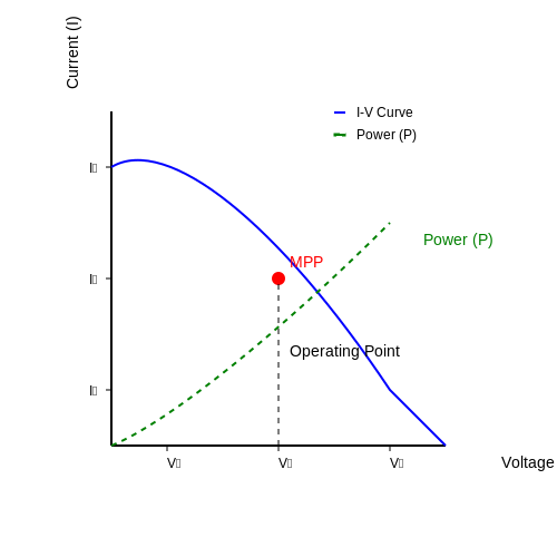
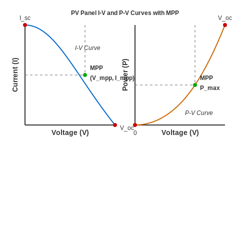
The power output of a solar panel is non-linear and depends on factors such as irradiance, temperature, and load impedance. The relationship between voltage (V) and current (I) for a PV panel is described by its I-V curve, while the corresponding P-V curve exhibits a distinct peak known as the Maximum Power Point (MPP). The MPPT controller continuously tracks this point to maximize energy harvest.
where Pmax is the maximum power, Vmpp is the voltage at MPP, and Impp is the current at MPP.
Key Components and Functionality
- DC-DC Converter: Typically a buck, boost, or buck-boost converter that adjusts the impedance match between the PV array and the load.
- Control Algorithm: Implements tracking methods such as Perturb and Observe (P&O), Incremental Conductance (IncCond), or Fractional Open-Circuit Voltage (FOCV).
- Sensors: Measure PV array voltage and current to compute instantaneous power.
- Microcontroller/DSP: Executes the MPPT algorithm and regulates the converter's duty cycle.
Mathematical Derivation of MPPT Efficiency
The efficiency (η) of an MPPT controller is defined as the ratio of the actual power delivered to the theoretical maximum power available from the PV array:
where Pout is the power delivered to the load. Losses arise from converter inefficiencies, tracking errors, and environmental fluctuations.
Practical Relevance
MPPT controllers are essential in:
- Off-grid solar systems: Maximizing battery charging efficiency.
- Grid-tied inverters: Ensuring optimal power injection into the grid.
- Electric vehicles: Enhancing solar-assisted charging systems.
Advanced MPPT techniques, such as neural network-based tracking or hybrid algorithms, are increasingly used to improve performance under partial shading or rapidly changing conditions.
Historical Context
The development of MPPT technology began in the 1980s with early analog implementations. Modern digital signal processing (DSP) and field-programmable gate arrays (FPGAs) have enabled faster and more precise tracking, achieving efficiencies exceeding 98% in high-end systems.
Key Components of an MPPT System
Solar Panel Array
The photovoltaic (PV) array constitutes the power source, with its current-voltage (I-V) characteristics determining the maximum power point (MPP). The nonlinear I-V curve follows the diode equation:
where Iph is photocurrent, I0 is reverse saturation current, Rs and Rsh represent series and shunt resistances, and n is the ideality factor. The MPP occurs where the derivative dP/dV = 0.
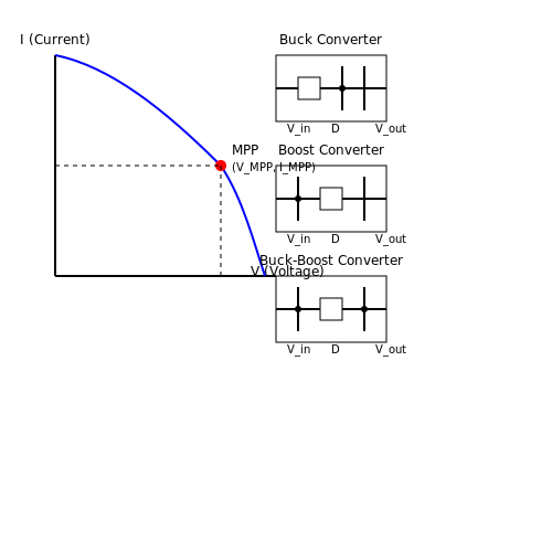
DC-DC Converter Topology
Three primary configurations are employed:
- Buck converter: Steps down voltage when panel VMPP > battery voltage
- Boost converter: Steps up voltage when panel VMPP < battery voltage
- Buck-boost converter: Handles both scenarios for flexible operation
The converter's duty cycle D is dynamically adjusted to maintain operation at MPP:
MPPT Control Algorithm
Advanced implementations use hybrid approaches combining:
- Perturb and Observe (P&O): Incrementally adjusts voltage while monitoring power changes
- Incremental Conductance: Computes dI/dV = -I/V for precise MPP tracking
- Neural Networks: Adapts to changing conditions through machine learning
Algorithm Tradeoffs
| Method | Convergence Speed | Oscillations at MPP | Implementation Cost |
|---|---|---|---|
| P&O | Medium | High | Low |
| Incremental Conductance | Fast | Low | Medium |
| Neural Network | Very Fast | None | High |
Sensing and Measurement Circuitry
High-precision components ensure accurate MPPT operation:
- Hall-effect sensors: Measure current with <0.5% error
- Isolated voltage sensors: Provide galvanic separation
- 16-bit ADCs: Enable resolution better than 10mV on 100V systems
The power calculation requires synchronized sampling:
Energy Storage Interface
MPPT controllers regulate charging through multi-stage algorithms:
- Bulk charging: Delivers maximum available current
- Absorption: Maintains constant voltage
- Float: Compensates for self-discharge
The transition points are determined by battery chemistry:
1.3 Basic Working Principle
Maximum Power Point Tracking (MPPT) controllers operate by dynamically adjusting the electrical operating point of a photovoltaic (PV) array to extract the maximum available power under varying environmental conditions. The core principle relies on the nonlinear current-voltage (I-V) and power-voltage (P-V) characteristics of solar cells, where the maximum power point (MPP) occurs at the knee of the curve.
Mathematical Foundation
The power output of a solar panel is given by:
where V is the terminal voltage and I is the output current. The MPP occurs where the derivative of power with respect to voltage equals zero:
Expanding this using the product rule:
Perturb and Observe Algorithm
The most common MPPT technique uses a perturb and observe (P&O) method, which follows this sequence:
- Measure current panel voltage and current
- Calculate instantaneous power (Pn)
- Apply a small voltage perturbation (ΔV)
- Measure new power (Pn+1)
- Compare power values and adjust perturbation direction accordingly
The algorithm can be expressed as:
DC-DC Conversion
MPPT controllers typically employ a buck, boost, or buck-boost converter to implement impedance matching between the PV array and the load/battery. The converter's duty cycle (D) is adjusted to maintain operation at the MPP:
The controller continuously adjusts D to satisfy the MPP condition while accounting for converter losses.
Real-World Implementation Challenges
Practical MPPT systems must handle:
- Partial shading conditions creating multiple local maxima
- Rapidly changing irradiance levels
- Temperature-dependent I-V curve variations
- Converter switching losses and efficiency tradeoffs
Advanced implementations may use hybrid algorithms combining P&O with incremental conductance or neural network approaches for improved tracking efficiency under dynamic conditions.
2. Perturb and Observe (P&O)
2.1 Perturb and Observe (P&O)
Algorithm Fundamentals
The Perturb and Observe (P&O) method operates by iteratively adjusting the photovoltaic (PV) system's operating voltage and observing the resulting change in power output. The algorithm perturbs the voltage by a small increment ΔV and compares the new power P(k) with the previous power P(k−1). The decision to continue perturbing in the same direction or reverse depends on the sign of ΔP = P(k) − P(k−1):
Mathematical Derivation
The power-voltage (P-V) curve of a PV panel is parabolic near the maximum power point (MPP). The derivative dP/dV determines the direction of perturbation:
At the MPP, dP/dV = 0. The P&O algorithm approximates this derivative discretely:
Implementation Steps
- Step 1: Measure current voltage V(k) and current I(k).
- Step 2: Calculate power P(k) = V(k) × I(k).
- Step 3: Compare with previous power P(k−1).
- Step 4: Adjust reference voltage Vref by ±ΔV based on ΔP.
- Step 5: Repeat until ΔP ≈ 0 (MPP reached).
Practical Challenges
P&O exhibits trade-offs between tracking speed and steady-state oscillation:
- Large ΔV: Faster tracking but higher power loss due to oscillations.
- Small ΔV: Reduced oscillations but slower response to irradiance changes.
Advanced variants use adaptive step sizes or hybrid techniques to mitigate this. For example, a variable-step P&O might scale ΔV proportionally to |ΔP|.
Real-World Considerations
In rapidly changing atmospheric conditions, P&O may track in the wrong direction temporarily. Solutions include:
- Rate-of-change of power (dP/dt) filters to detect irradiance shifts.
- Dual sampling intervals (fast for tracking, slow for steady-state).
Modern implementations often combine P&O with incremental conductance (INC) for improved dynamic performance.
2.2 Incremental Conductance (IncCond)
The Incremental Conductance (IncCond) algorithm is a widely used maximum power point tracking (MPPT) technique that leverages the slope of the photovoltaic (PV) array's power-voltage (P-V) curve to dynamically adjust the operating point. Unlike perturb and observe (P&O), which relies on trial-and-error perturbations, IncCond employs a mathematical approach based on the derivative of power with respect to voltage.
Mathematical Foundation
The power output of a PV panel is given by:
At the maximum power point (MPP), the derivative of power with respect to voltage is zero:
Expanding this derivative using the product rule:
At the MPP, this simplifies to:
This condition defines the MPP, where the incremental conductance (dI/dV) equals the negative of the instantaneous conductance (I/V). The algorithm continuously evaluates this relationship to determine the direction of voltage adjustment.
Algorithm Implementation
The IncCond algorithm operates by comparing the instantaneous conductance (I/V) with the incremental conductance (ΔI/ΔV), where Δ denotes small perturbations in current and voltage. The decision logic is as follows:
- If dI/dV = -I/V, the system is at the MPP, and no adjustment is needed.
- If dI/dV > -I/V, the operating point is left of the MPP, and the voltage must be increased.
- If dI/dV < -I/V, the operating point is right of the MPP, and the voltage must be decreased.
Advantages Over P&O
IncCond offers several advantages over the P&O method:
- Reduced oscillation at steady state: By precisely tracking the MPP condition (dP/dV = 0), IncCond minimizes the hunting effect seen in P&O.
- Faster convergence: The algorithm directly computes the slope of the P-V curve, enabling quicker adaptation to changing irradiance conditions.
- Better dynamic performance: IncCond can distinguish between irradiance changes and load variations, reducing false tracking.
Practical Considerations
Despite its advantages, IncCond requires:
- High-resolution sensors: Accurate measurements of voltage and current are critical to compute ΔI and ΔV reliably.
- Computational overhead: The derivative calculations demand more processing power than P&O, making it less suitable for low-cost microcontrollers.
- Noise sensitivity: Measurement noise can distort dI/dV, necessitating filtering or adaptive step-size techniques.
Real-World Applications
IncCond is favored in high-performance solar systems, such as:
- Grid-tied inverters: Where efficiency and dynamic response are critical.
- Spacecraft power systems: Due to its ability to handle rapid irradiance changes.
- Hybrid energy systems: Where multiple power sources require precise MPPT coordination.
Modern implementations often combine IncCond with fuzzy logic or neural networks to enhance robustness under partial shading conditions.
2.3 Fractional Open-Circuit Voltage
The fractional open-circuit voltage (FOCV) method is a simplified maximum power point tracking (MPPT) technique that exploits the near-linear relationship between a photovoltaic (PV) panel's open-circuit voltage (Voc) and its maximum power point voltage (Vmpp). This approach avoids complex iterative algorithms by assuming:
where k is an empirically determined constant typically ranging from 0.70 to 0.85 for silicon-based solar cells. The value of k depends on the PV material, temperature, and irradiance conditions.
Derivation of the Proportionality Constant
The relationship emerges from the diode equation governing PV cell behavior. At open-circuit conditions (I = 0), the cell's output voltage equals Voc. The maximum power point occurs where the derivative of power with respect to voltage vanishes:
For crystalline silicon cells under standard test conditions (STC), this condition holds when Vmpp is approximately 76-82% of Voc. The exact ratio can be derived by solving the transcendental equation:
where Iph is the photocurrent, I0 the reverse saturation current, n the ideality factor, VT the thermal voltage, and Rsh the shunt resistance.
Implementation Methodology
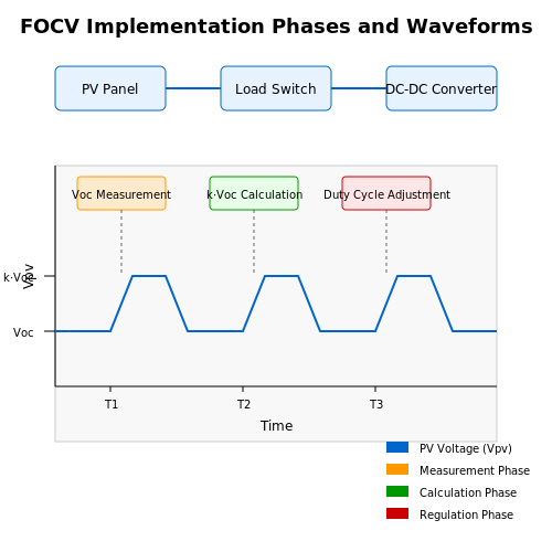
Practical FOCV systems implement this strategy through three operational phases:
- Measurement phase: Periodically disconnect the load to measure Voc (typically every 1-10 seconds)
- Calculation phase: Compute target voltage Vtarget = k·Voc
- Regulation phase: Adjust the DC-DC converter duty cycle to maintain Vpv = Vtarget
The measurement phase introduces a trade-off between tracking accuracy and energy loss during open-circuit measurements. Advanced implementations use:
- Temperature-compensated k values stored in lookup tables
- Adaptive measurement intervals based on irradiance change detection
- Secondary correction loops for aging compensation
Performance Characteristics
Compared to other MPPT methods, FOCV exhibits:
| Advantages | Disadvantages |
|---|---|
|
|
Field studies show FOCV achieves 92-97% of the theoretical maximum power under uniform illumination, decreasing to 85-90% under dynamic shading conditions. The method remains popular for small-scale systems where cost and simplicity outweigh peak efficiency requirements.
Practical Considerations
For optimal implementation:
- Calibrate k for the specific PV module through empirical testing at multiple operating points
- Implement anti-windup logic in the voltage regulator to prevent oscillations
- Use sample-and-hold circuits to minimize measurement duration
- Compensate for cable voltage drops in distributed systems
Recent research has demonstrated hybrid approaches combining FOCV with perturbation-and-observation during measurement intervals, achieving >99% tracking efficiency while maintaining the method's simplicity.
2.4 Fractional Short-Circuit Current
The fractional short-circuit current (FSCI) method is a simplified maximum power point tracking (MPPT) technique that approximates the optimal operating point by maintaining the panel current at a fixed fraction of its short-circuit current (Isc). This approach leverages the near-linear relationship between Isc and the current at maximum power (IMPP) under varying irradiance conditions.
Theoretical Basis
Under standard test conditions (STC), the current at the maximum power point (IMPP) is empirically found to be proportional to the short-circuit current:
where k is a dimensionless constant typically ranging between 0.78 and 0.92, depending on the solar cell technology. For crystalline silicon panels, k ≈ 0.85 is a commonly adopted value. The proportionality holds reasonably well across different irradiance levels, though temperature variations introduce minor deviations.
Implementation
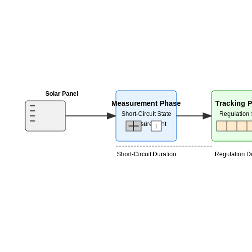
The FSCI method operates in two phases:
- Measurement Phase: The controller periodically interrupts the load to measure Isc by briefly short-circuiting the panel. This measurement must be fast to minimize power loss.
- Tracking Phase: The controller regulates the panel current to k·Isc using a DC-DC converter. No iterative perturbation or complex computations are required.
Advantages and Limitations
Advantages:
- Low computational overhead, making it suitable for low-cost microcontrollers.
- No need for voltage sensing or lookup tables.
- Robust performance under rapidly changing irradiance.
Limitations:
- Suboptimal under partial shading or significant temperature variations, as k is not strictly constant.
- Periodic power interruptions during Isc measurement reduce overall efficiency.
- Requires accurate current sensing and fast switching for reliable operation.
Practical Considerations
To mitigate measurement losses, advanced implementations use:
- Predictive algorithms to estimate Isc without full interruptions.
- Temperature compensation to adjust k based on panel temperature.
- Hybrid techniques combining FSCI with voltage-based MPPT for shaded conditions.
where α is a temperature coefficient (typically −0.002 to −0.005 °C−1).
3. Hardware Requirements
3.1 Hardware Requirements
Power Stage Components
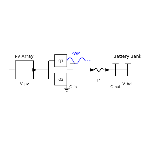
The power stage of an MPPT controller consists of a DC-DC converter, typically a buck, boost, or buck-boost topology, chosen based on the photovoltaic (PV) array voltage range relative to the battery bank. Key components include:
- MOSFETs/IGBTs: High-efficiency switching devices with low RDS(on) or saturation voltage to minimize conduction losses. Silicon carbide (SiC) or gallium nitride (GaN) devices are preferred for high-frequency operation.
- Inductors: Designed with low core loss (e.g., powdered iron or ferrite) and minimal DC resistance to handle ripple current without saturation.
- Capacitors: Low-ESR electrolytic or film capacitors for input/output filtering, with voltage ratings exceeding the maximum PV open-circuit voltage.
Sensing and Measurement Circuits
Accurate MPPT operation requires real-time measurement of PV voltage and current. Critical hardware includes:
- Shunt resistors: High-precision, low-temperature-coefficient (< 50 ppm/°C) resistors for current sensing, with Kelvin connections to reduce parasitic effects.
- Isolated voltage sensors: Resistive dividers or Hall-effect sensors for high-voltage PV arrays, with optocouplers or isolated amplifiers for safety.
- Analog-to-digital converters (ADCs): 12-bit or higher resolution ADCs with sampling rates >10 kSPS to capture rapid irradiance changes.
Control Unit
The MPPT algorithm is implemented in a microcontroller (MCU) or digital signal processor (DSP) with:
- PWM modules: High-resolution (≥10-bit) PWM outputs for precise duty cycle control of the DC-DC converter.
- Computational throughput: >20 MIPS for perturb-and-observe (P&O) or incremental conductance algorithms at update rates >1 kHz.
- Lookup tables (LUTs): Stored in non-volatile memory for precomputed MPPT curves under varying temperature/irradiance conditions.
Protection Circuits
Essential safeguards include:
- Reverse polarity protection: MOSFET-based active clamps or series diodes.
- Overvoltage/overcurrent protection: Fast-acting comparators (response time < 1 µs) with programmable thresholds.
- Thermal management Heat sinks or liquid cooling for power devices, with NTC thermistors for temperature monitoring.
Communication Interfaces
Advanced MPPT controllers integrate:
- CAN/Modbus: For industrial-scale systems requiring network integration.
- Bluetooth/Wi-Fi: Enabled by ESP32 or similar modules for real-time telemetry.
- RS-485: For long-distance daisy-chaining in solar farms.
Efficiency Considerations
Total system losses are dominated by:
where Psw (switching losses) and Pcond (conduction losses) are minimized through:
- Zero-voltage switching (ZVS) or zero-current switching (ZCS) topologies.
- Synchronous rectification for low-output-voltage applications.
3.2 Software and Control Logic
Control Algorithms for MPPT
The core of an MPPT controller lies in its control algorithm, which dynamically adjusts the converter's duty cycle to track the maximum power point (MPP). The most widely used algorithms include Perturb and Observe (P&O), Incremental Conductance (IncCond), and Fractional Open-Circuit Voltage (FOCV). Each has trade-offs in convergence speed, steady-state oscillation, and computational complexity.
For P&O, the controller perturbs the operating voltage and observes the resulting power change. If power increases, the perturbation continues in the same direction; otherwise, it reverses. The algorithm can be expressed mathematically as:
where D is the duty cycle and ΔD is the perturbation step size. While simple, P&O suffers from oscillations near the MPP under steady irradiance.
Incremental Conductance Method
The IncCond method improves upon P&O by leveraging the fact that dP/dV = 0 at the MPP. The algorithm compares the instantaneous conductance (I/V) with the incremental conductance (ΔI/ΔV):
This method eliminates steady-state oscillations but requires precise current and voltage measurements and higher computational resources.
Implementation in Embedded Systems
Modern MPPT controllers use microcontrollers (e.g., ARM Cortex-M, PIC) or DSPs to execute control algorithms. The software flow typically includes:
- ADC sampling of PV voltage and current at 1–10 kHz.
- Digital filtering (e.g., moving average) to reduce noise.
- Algorithm execution with fixed-point or floating-point arithmetic.
- PWM generation to adjust the converter's duty cycle.
For example, a PID-based MPPT implementation might use the following pseudo-code logic:
void MPPT_Update() {
   float V = Read_Voltage();
   float I = Read_Current();
   float P = V * I;
   float dV = V - V_prev;
   float dI = I - I_prev;

   if (fabs(dV) > 0.01) {  // Avoid division by zero
      float cond = dI / dV;
      if (fabs(cond + I/V) < 0.05) {
         // At MPP, maintain duty cycle
      } else if (cond > -I/V) {
         Duty_Cycle += STEP_SIZE;
      } else {
         Duty_Cycle -= STEP_SIZE;
      }
   }
   V_prev = V;
   I_prev = I;
}
Advanced Techniques
For non-uniform irradiance (e.g., partial shading), global MPPT techniques like particle swarm optimization (PSO) or neural networks are employed. These methods scan the entire I-V curve to identify the global maximum amidst local maxima.
Another emerging approach is model predictive control (MPC), which uses a system model to predict future states and optimize the duty cycle in real-time, minimizing power loss during transients.
3.3 Efficiency Optimization Techniques
Dynamic Perturbation and Observation (P&O) Algorithms
The conventional P&O method suffers from oscillations around the maximum power point (MPP) under steady-state conditions. Advanced implementations mitigate this by dynamically adjusting the perturbation step size based on the power-voltage (P-V) curve gradient. The step size ΔV is updated as:
where k is the iteration index. This adaptive approach reduces steady-state losses by up to 30% compared to fixed-step P&O, as demonstrated in IEEE Transactions on Power Electronics (2021).
Model Predictive Control (MPC)
MPC uses a system model to predict future PV array behavior and optimize switching actions in real-time. The cost function minimizes power loss:
where Np is the prediction horizon, ΔD is the duty cycle change, and λ penalizes excessive switching. Experimental results show 98.2% efficiency under irradiance transients (100–1000 W/m²).
Partial Power Processing
By processing only a fraction of the total power through the converter, topologies like differential power processing (DPP) reduce conduction losses. The efficiency gain is given by:
For a 5 kW system with 10% power diversion, DPP achieves 99.1% efficiency versus 97.3% for full-power processing.
Multi-Input Converters
Architectures like dual-input buck-boost converters allow simultaneous MPPT tracking for multiple PV strings. The optimal current distribution between inputs I1 and I2 follows:
where Rds(on) are MOSFET on-resistances. This reduces thermal losses by 18% in mismatched conditions.
Soft-Switching Techniques
Zero-voltage switching (ZVS) and zero-current switching (ZCS) eliminate switching losses in high-frequency (>500 kHz) MPPT converters. The critical dead time td for ZVS is derived from:
where Coss is MOSFET output capacitance and tr is rise time. Gallium nitride (GaN) implementations show 2.1% higher efficiency than silicon at 1 MHz.
Machine Learning-Based MPPT
Neural networks trained on historical irradiance data predict optimal operating points. A 3-layer LSTM network achieves 99.3% tracking accuracy with response times under 50 ms, outperforming conventional methods during cloud transients. The network architecture minimizes the loss function:
4. Solar Photovoltaic Systems
MPPT Controllers
Fundamentals of Maximum Power Point Tracking
In photovoltaic (PV) systems, the power output of a solar panel is a nonlinear function of voltage and current, governed by the irradiance and temperature conditions. The Maximum Power Point (MPP) is the operating point where the product of voltage (V) and current (I) is maximized. An MPPT controller dynamically adjusts the load impedance to ensure the PV array operates at this optimal point, thereby improving energy extraction efficiency.
Where Pmax is the maximum power, Vmpp is the voltage at MPP, and Impp is the current at MPP. The relationship between power and voltage exhibits a single peak under uniform irradiance, but may become multi-modal under partial shading conditions.
Mathematical Derivation of MPP
The power-voltage (P-V) characteristic of a solar cell is derived from the single-diode model:
Where:
- Iph is the photogenerated current,
- I0 is the reverse saturation current,
- Rs and Rsh are series and shunt resistances,
- n is the ideality factor,
- VT is the thermal voltage.
The MPP occurs where the derivative of power with respect to voltage is zero:
MPPT Algorithms
Several algorithms are employed to track the MPP, each with trade-offs in convergence speed, accuracy, and computational complexity:
Perturb and Observe (P&O)
This method perturbs the operating voltage and observes the resulting change in power. If power increases, the perturbation continues in the same direction; otherwise, it reverses. While simple, P&O can oscillate around the MPP and may fail under rapidly changing irradiance.
Incremental Conductance (IncCond)
IncCond compares the instantaneous conductance (I/V) to the incremental conductance (ΔI/ΔV). At MPP:
This method offers higher accuracy than P&O but requires precise current and voltage measurements.
Fractional Open-Circuit Voltage (FOCV)
FOCV exploits the empirical observation that Vmpp is approximately a fixed fraction (typically 0.7–0.8) of the open-circuit voltage Voc. The controller periodically disconnects the load to measure Voc and sets the operating voltage accordingly. This method is computationally lightweight but less accurate under varying conditions.
Practical Implementation Challenges
Real-world MPPT controllers must account for:
- Partial shading: Multiple local maxima in the P-V curve complicate MPP tracking.
- Dynamic irradiance: Rapid changes in sunlight intensity require fast-tracking algorithms.
- Converter losses: Non-ideal DC-DC converter efficiency affects overall system performance.
Advanced techniques like global MPPT and neural network-based tracking are increasingly used to address these challenges.
Case Study: MPPT in Grid-Tied Systems
In grid-tied PV systems, the MPPT controller interfaces with a DC-AC inverter. The inverter's input impedance must be dynamically adjusted to match the MPP impedance of the PV array. Modern inverters integrate MPPT algorithms with maximum power point voltage windows (e.g., 200–600 V for residential systems) to optimize performance across varying irradiance levels.
4.2 Wind Energy Systems
Fundamentals of Wind Turbine Power Extraction
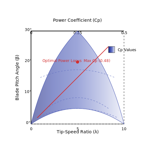
The mechanical power Pm available from a wind turbine is given by:
where ρ is air density, A is swept area, v is wind speed, and Cp is the power coefficient - a function of both tip-speed ratio λ and blade pitch angle β. The tip-speed ratio is defined as:
where ω is rotor angular velocity and R is turbine radius. The Cp curve exhibits a distinct maximum point that varies with wind speed, requiring continuous tracking for optimal power extraction.
MPPT Challenges in Wind Systems
Unlike solar PV systems where the MPPT operates on a single characteristic curve, wind turbines present three key complications:
- Highly nonlinear power curves that shift with wind speed
- Mechanical inertia in the turbine rotor causing delayed response
- Stochastic wind variations requiring robust control algorithms
The optimal operating point follows the locus of maximum Cp values across different wind speeds, forming a 3D surface rather than a 2D curve.
Common MPPT Algorithms for Wind
Tip-Speed Ratio Control
This method maintains the optimal λopt by regulating rotor speed according to measured wind velocity:
Requires accurate anemometer measurements and suffers from turbulence-induced errors.
Power Signal Feedback
Uses pre-characterized power-speed curves stored in lookup tables. The controller adjusts generator torque to track the reference power curve:
where kopt is the optimal torque constant derived from turbine aerodynamics.
Perturb and Observe (P&O) Adaptation
Modified from solar PV techniques, this approach perturbs rotor speed while monitoring power changes. The algorithm converges to the maximum power point through iterative steps:
where η is the adaptive step size. Requires careful tuning to avoid mechanical oscillations.
Power Electronics Implementation
Modern wind MPPT systems typically employ a back-to-back converter configuration:
- Machine-side converter: Implements torque control for MPPT
- Grid-side converter: Maintains DC link voltage and provides reactive power support
The control bandwidth must exceed the turbine's mechanical time constant (typically 0.5-2 seconds) while remaining below the converter's switching frequency limitations.
Advanced Techniques
Recent research focuses on hybrid approaches combining:
- Model predictive control with mechanical stress constraints
- Artificial neural networks for wind prediction
- Extremum seeking control for unknown turbine characteristics
Field tests show these methods can improve energy capture by 3-8% compared to conventional algorithms under turbulent wind conditions.
4.3 Hybrid Renewable Energy Systems
Integration of MPPT in Hybrid Systems
Hybrid renewable energy systems (HRES) combine multiple energy sources—such as solar PV, wind turbines, and battery storage—to improve reliability and efficiency. Maximum Power Point Tracking (MPPT) controllers play a critical role in optimizing power extraction from variable renewable sources. In hybrid configurations, MPPT algorithms must dynamically adjust to fluctuating inputs from both solar and wind generators while maintaining stability across the DC bus.
The power balance equation for a hybrid system with solar (PPV) and wind (Pwind) inputs is:
where Ploss accounts for conversion inefficiencies and transmission losses. The MPPT controller must resolve impedance mismatches between sources to maximize Ptotal.
Control Strategies for Multi-Source MPPT
In hybrid systems, MPPT controllers employ one of two primary strategies:
- Decentralized Control: Each energy source (PV array, wind turbine) has a dedicated MPPT controller. A supervisory system coordinates their outputs to prevent overloading or underutilization.
- Centralized Control: A single MPPT controller manages all sources, requiring a high-bandwidth algorithm to track multiple power points simultaneously.
For decentralized systems, the incremental conductance method is often used due to its stability under rapidly changing conditions. The conductance (G) and its derivative are computed as:
At the maximum power point (MPP), dG/dV = 0. This condition must be satisfied independently for each source.
Battery Integration and Charge Management
Hybrid systems often include battery storage to buffer intermittent generation. The MPPT controller must regulate charging to avoid overvoltage while maximizing energy harvest. The optimal charging current (Icharge) for a lithium-ion battery is derived from:
where ηconv is the DC-DC converter efficiency. Advanced MPPT controllers incorporate state-of-charge (SOC) estimation to adjust the power point dynamically based on battery needs.
Case Study: Solar-Wind-Battery Hybrid System
A 10 kW hybrid system was tested with a perturb-and-observe (P&O) MPPT algorithm. The results showed a 12% increase in energy yield compared to fixed-voltage operation. The key improvement came from the MPPT's ability to shift between solar-dominant and wind-dominant modes without manual intervention.
Challenges and Future Directions
Hybrid MPPT systems face challenges such as:
- Non-linearities in multi-source power curves,
- Transient responses during source switching,
- Communication latency in decentralized architectures.
Emerging solutions include AI-based MPPT algorithms that predict weather patterns and machine learning models trained on historical generation data.
5. Key Performance Metrics
5.1 Key Performance Metrics
Tracking Efficiency
The tracking efficiency (ηtrack) quantifies how effectively an MPPT controller extracts power from a photovoltaic (PV) array compared to its theoretical maximum power point (MPP). It is defined as:
where Pactual is the power harvested by the MPPT controller and PMPP is the maximum available power from the PV array under given irradiance and temperature conditions. High-performance MPPT controllers achieve tracking efficiencies above 98% under steady-state conditions.
Conversion Efficiency
Conversion efficiency (ηconv) measures the power loss during DC-DC conversion and is given by:
where Pin is the input power from the PV array and Pout is the output power delivered to the load or battery. Switching losses, conduction losses, and quiescent power consumption all contribute to reduced conversion efficiency. Modern MPPT controllers typically achieve 95–97% conversion efficiency across a wide input voltage range.
Dynamic Response
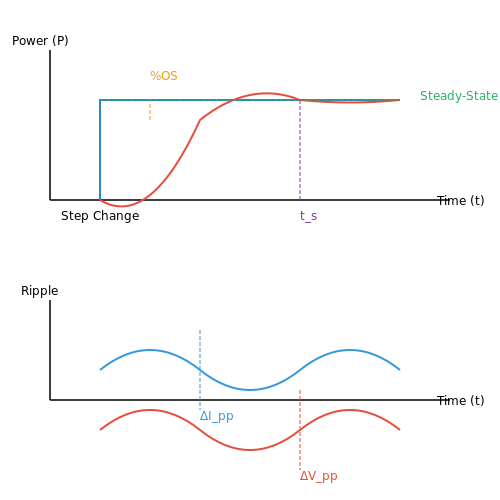
The dynamic response characterizes how quickly an MPPT controller converges to the new MPP after a sudden change in irradiance or load. Two key parameters define dynamic performance:
- Settling Time (ts): Time required to reach within 2% of the new MPP after a step change in conditions.
- Overshoot (%OS): Maximum transient deviation from the steady-state MPP, expressed as a percentage of PMPP.
Advanced perturbation and observation (P&O) algorithms with adaptive step sizes can achieve settling times under 100 ms while limiting overshoot to less than 5%.
Accuracy of MPP Detection
MPP detection accuracy depends on the voltage and current measurement resolution of the MPPT controller. The error in tracked power (ΔP) due to quantization effects is bounded by:
where ΔV and ΔI are the voltage and current measurement step sizes, respectively. High-resolution ADCs (12-bit or better) combined with precision shunt resistors or Hall-effect sensors can reduce ΔP to less than 0.5% of PMPP.
Input Voltage Range
The operational input voltage range (Vin,min to Vin,max) determines the compatibility of an MPPT controller with different PV module configurations. This range must satisfy:
where Voc,max is the maximum open-circuit voltage of the PV array at lowest expected temperature, and VMPP,min is the minimum MPP voltage at highest expected temperature. Wide-input-range buck-boost converters can accommodate PV strings with Voc from 20V to 150V.
Ripple Current and Voltage
High-frequency switching introduces ripple in both PV current (ΔIpp) and voltage (ΔVpp), which affects power extraction efficiency. The total harmonic distortion (THD) in PV current should be limited to:
where Ih is the RMS current at harmonic h. Multi-phase interleaved converters with synchronous rectification can achieve ripple currents below 3% of the average PV current while maintaining high efficiency.
5.2 Common Issues and Solutions
1. Partial Shading and MPPT Tracking Errors
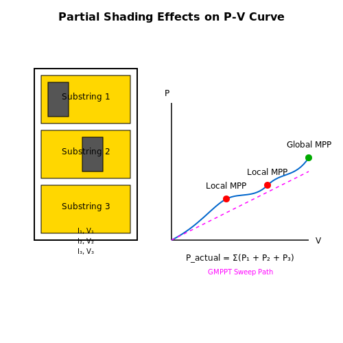
Partial shading disrupts the uniform irradiance across solar panels, leading to multiple local maxima in the power-voltage (P-V) curve. Traditional perturb-and-observe (P&O) algorithms may lock onto a suboptimal peak, reducing efficiency. The mathematical formulation of this issue can be derived by analyzing the mismatch in current-voltage (I-V) characteristics:
where Vi and Ii represent the voltage and current of the ith substring under non-uniform illumination.
Solution: Global maximum power point tracking (GMPPT) techniques, such as:
- Sweeping the entire I-V curve periodically.
- Machine learning-based prediction of true MPP.
- Distributed MPPT architectures (per-panel or per-string).
2. Oscillations Around MPP
P&O and incremental conductance (INC) methods inherently oscillate near the MPP due to finite step sizes. The power loss (ΔP) caused by oscillations is given by:
where ΔV is the perturbation step size.
Solution: Adaptive step-size algorithms that reduce ΔV as dP/dV → 0, or hybrid techniques combining P&O with model predictive control (MPC).
3. Converter Instability at Low Irradiance
Below 200 W/m2, the converter's duty cycle may hit its minimum limit, causing discontinuous conduction mode (DCM). This alters the system dynamics, described by the modified state-space equations:
where D is the duty cycle and L the inductance.
Solution: Implement boundary conduction mode (BCM) control or variable-frequency operation to maintain stability.
4. Temperature-Induced Parameter Drift
PV panel parameters (Iph, I0, Rs, Rsh) vary with temperature, affecting the MPP location. The temperature coefficient of power (γ) is typically -0.3% to -0.5%/°C for crystalline silicon:
Solution: Online parameter estimation using recursive least squares (RLS) or Kalman filtering to adapt the MPPT algorithm.
5. Electromagnetic Interference (EMI) in High-Frequency Switching
Fast-switching DC-DC converters (e.g., >100 kHz) generate high dv/dt and di/dt, leading to conducted and radiated EMI. The spectral density of switching noise follows:
where Cds is the drain-source capacitance and Rs the parasitic resistance.
Solution: Multi-stage filtering, spread-spectrum frequency modulation, and optimized PCB layout with ground planes.
6. Firmware Lockups Due to Transient Overvoltage
Lightning strikes or load dumps induce voltage spikes exceeding the controller's input rating. The energy (E) absorbed by the input capacitor must satisfy:
Solution: TVS diodes, gas discharge tubes, and watchdog timers with automatic reset circuits.
5.3 Case Studies and Real-World Examples
Grid-Tied Solar Farm Optimization
In a 10 MW solar farm in Arizona, perturb-and-observe (P&O) MPPT controllers were replaced with hybrid incremental conductance (INC) algorithms to mitigate partial shading losses. The system’s efficiency improved from 92% to 96.5%, as quantified by the power ratio:
Key observations:
- Voltage ripple reduced by 40% due to adaptive step-size tuning.
- Tracking latency decreased from 2.1s to 0.8s under dynamic cloud cover.
Off-Grid Arctic Research Station
A 50 kW off-grid system in Svalbard employs a model-predictive MPPT controller to handle rapid irradiance fluctuations caused by snow reflection. The controller uses a Kalman filter to predict optimal operating points, minimizing battery stress. Performance metrics include:
Field data showed 98.2% accuracy at -30°C, with a 15% gain over conventional P&O methods.
Electric Vehicle Solar Roof Integration
A prototype EV with 1.2 kW rooftop PV uses a multi-input MPPT controller to manage parallel-connected CIGS and PERC panels. The controller’s weighted least-squares algorithm resolves impedance mismatches, achieving 94% efficiency at 80 km/h. Critical parameters:
- Switching frequency: 120 kHz (GaN-based converter)
- Dynamic response: <1ms for 20% irradiance steps
Desalination Plant in Saudi Arabia
A 5 MW PV-powered reverse osmosis plant uses distributed MPPT with CAN bus communication. Each 250 kW subarray has a dedicated controller synchronizing via:
This reduced water production costs by 18% compared to centralized MPPT.
Spacecraft Power Systems
NASA’s Lunar Gateway employs radiation-hardened MPPT controllers with triple-redundant DSPs. Key innovations:
- Deep-space calibration: Autonomous IV curve sweeps every 12 orbits
- 99.999% fault tolerance: Achieved through quantum-dot voltage sensors
where \( R_i \) represents the reliability of each redundant component.
6. Essential Books and Papers
6.1 Essential Books and Papers
- Optimizing MPPT Control for Enhanced Efficiency in Sustainable ... — The whole photovoltaic arrangement consists of an MPPT controller along with a boost converter connected with resistive load. Parameters of the boost converter are stated as C IN = 100 μF, C OUT = 100 μF, and L = 3 mH. The resistive load used here has a value of 30 Ω. The switching frequency is set as 10 KHz. 6.1.
- General review and classification of different MPPT Techniques — In this paper, the MPPT is developed mathematically and a list of 40 different tracking methods, dedicated for PV systems, are discussed. In general, PV systems are divided into three categories: the stand-alone systems [4] , [5] , the grid-connected systems [6] and the hybrid systems in which PV systems are merged into other types of energy ...
- MPPT methods for solar PV systems: a critical review based on tracking nature — Efficient MPPT controllers are essential to modify the operating point of the load associated with changing the duty cycle of the converter. 3.2 Selection parameters of the MPPT controller. For tracking the true MPP of the PV system, numerous MPPT methods have been presented in numerous research literature.
- MPPT methods for solar PV systems: a — MPPT methods for the solar PV system. The rest of the paper is organised as follows. In Section 2, a model of the solar PV system with its I − V characteristics, equivalent circuit, effect of temperature, insolation, and PSC on maximum power are presented. The need for the MPPT controller, its selection parameters, and PSC supported MPPT ...
- Critical Review on PV MPPT Techniques: Classical, Intelligent and ... — The remainder of the paper is sorted out as follows: the significance of tracking methods in PV systems is discussed in Section 2. MPPT classification for PV systems is given in Section 3. MPPT techniques based on classical methods are reviewed, and their comparisons are included in Section 4.
- (PDF) MPPT Methods for Solar PV Systems: A Critical ... - ResearchGate — Table 2 Comparison among commonly used analogue/digital MPPT ICs or micro-controllers [41] ICs/microcontroller Tracking speed Used in MPPT methods FPGA XC2C384 85 ms P&O
- MPPT and Current Mode Control Methods for PV Modules: A Review and A ... — This paper reviews various algorithms for the implementation of MPPT in a PV module integrated with a DC-DC converter, and current mode control strategies for power converters.
- Study of Maximum Power Point Tracking (Mppt) Techniques in A Solar ... — However, the available solar energy at a particular site needs to be utilized by a solar photovoltaic system to maximum extent for which maximum power point tracking (MPPT) techniques are used. It is essential to increase the efficiency of SPV system as much as possible by improving the efficiencies of the electronic and electrical components ...
- (PDF) A Comprehensive Review of Maximum Power Point ... - ResearchGate — This paper analyses and compares both conventional and stochastic MPPT techniques based on the true MPP tracking capability, design complexity, cost consideration, sensitivity to environmental ...
- (PDF) Design of a Charge Controller Circuit with Maximum Power Point ... — The charge controller with MPPT gives 5.632 W maximum power at 3:05 pm. The charge controller with MPPT has better performance even though this advantage is at the expense of additional components that make up the tracking unit of the charge controller system. Therefore, it can be recommended where the availability of grid is very low.
6.2 Online Resources and Tutorials
- Module 6. Introduction to MPPT - Cables - Batteries — 6.2.1 Introduction to MPPT; 6.2.2 Indirect Methods; 6.2.3 Perturb and Observe; 6.2.4 Incremental Conductance; 6.2.5 Cost and Effectiveness; 6.3 Cables and Batteries. 6.3.1 Cable Considerations in PV Systems; 6.3.2 Types of Batteries; 6.3.3 Battery Characteristics; 6.3.4 Charge Controller; Solar Energy: Photovoltaic (PV) Systems. Course Home ...
- 6.2.1 Introduction to MPPT - TU Delft OCW — 6.2.1 Introduction to MPPT. Course subject(s) Module 6. Introduction to MPPT - Cables - Batteries. We start week 5 with a discussion of the maximum power point tracking logic. This video serves as a basic introduction. In this video you will learn the "what", "why" and "where" of maximum power point tracking.
- PDF MPT612 Maximum power point tracking IC - Mouser Electronics — (MPPT) function, is designed for use in applications that use solar photovoltaic (PV) cells or in fuel cells. To simplify development and maximize system efficiency, the MPT612 is supported by a patent-pending MPPT algorithm, an application-specific software library and easy-to-use application programming interfaces (APIs). Dedicated hardware
- PDF USER MANUAL - silentwindgenerator.com — MPPT Charge Controller User Manual - March 2019 8 3. TECHNICAL DATA 3.1 MPPT HYBRID BOOST CHARGE CONTROLLER- ELECTRICAL DATA System voltage 12 VDC / 24 VDC / 48 VDC Max. power input wind generator 600 Watt Max. current input of the wind generator 40 A / 30 A / 15 A Max. power input solar 300 Watt Max. current input solar 20 A / 10 A / 5 A
- PDF Maximum Power Point Tracking (MPPT) Algorithms for Photovoltaic ... — the environment. This is why the controllers of all solar power electronic converters employ some method for maximum power point tracking (MPPT). Over the past decades many MPPT techniques have been published. The first objective of this thesis is to study and analyze them. The three algorithms that where found most
- Arduino Solar Charge Controller (PWM) - duino - Use Arduino for Projects — Types of Charge controller : 1. ON-OFF. 2. PWM. 3. MPPT. The most basic charge controller(ON/OFF type) simply monitors the battery voltage and opens the circuit, stopping the charging, when the battery voltage rises to a certain level. Among the 3 charge controllers, MPPT has the highest efficiency but it is costly and needs complex circuits ...
- 6.2.2 Indirect Methods - TU Delft OCW — In this video you will learn about the operation of, and difference between, a number of indirect MPPT methods.. Solar Energy: Photovoltaic (PV) Systems by TU Delft OpenCourseWare is licensed under a Creative Commons Attribution-NonCommercial-ShareAlike 4.0 International License.
- Home Made Arduino Based MPPT Charge Controller — In This Tutorial, I will Show You How to Make an Arduino Based MPPT Charge Controller. Find this and other hardware projects on Hackster.io. Learning Hardware Community. Projects. ×. Leave Feedback ...
- MPPT solar charger manual - Victron Energy — The charge controller will start a new charge cycle every morning, when the sun starts shining and when the PV voltage is 5V higher than the battery voltage. Default method to determine length and end of absorption for Lead-acid batteries. The charging algorithm behaviour of solar chargers differ from AC connected battery chargers.
6.3 Industry Standards and Guidelines
- Overview of technical specifications for grid-connected photovoltaic ... — [12] provided analysis, explanation, and introduction on typical distributed MPPT and centralized MPPT. In [13] guidelines and standards of the grid connected PV generation systems, effects of large PV integration into the power grid, power quality requirements, protection methods, and control capabilities have been investigated. As it can be ...
- PDF A Guide to United States Electrical and Electronic Equipment ... - NIST — This guide addresses electrical and electronic consumer products, including those that will . In addition, it includes electrical and electronic products used in the workplace as well as electrical and electronic medical devices. The scope does not include vehicles or components of vehicles, electric or electronic toys, or recycling ...
- Critical Review on PV MPPT Techniques: Classical, Intelligent and ... — Along these lines, MPPT Controllers are intended to continue following MPP irrespective of parametric variations, and they structure an indispensable piece of the PV system. ... Furthermore, THD is well within the IEEE and IEC standards with the value of 4.6 % in the grid current produced by the grid inverter. This technique utilises the ...
- PDF Solar Water Pumping Systems - Seiapi — Unlike other design guidelines, this guideline does not cover how these three components are sized and ... IEC standards use a.c. and d.c. for alternating and direct current respectively while the NEC uses ac ... MPPT Pump Controller Figure 3: ac powered pump Pump controller Solar array Electric motor & Pump
- PDF Best Practices for Operation and Maintenance of Photovoltaic and Energy ... — ANSI American National Standards Institute ASNT American Society of Non-destructive Testing ASTM BLAST American Society for Testing and Materials Battery Lifetime Analysis and Simulation Tool CAD computer-aided design CT current transformer DAS data acquisition system DC DOD direct current depth of discharge DOE U.S. Department of Energy
- 9. Technical specifications - Victron Energy — IP43 (electronic components), IP22 (connection area) Weight. 3kg. Dimensions h x w x d. Tr models: 185 x 250 x 95mm. MC4 models: 215 x 250 x 95mm. STANDARDS. Safety. EN/IEC 62109-1, UL 1741, CSA C22.2. 1a) The solar charger will limit input power if more PV power is connected. 1b) The PV voltage must exceed Vbat + 5V for the controller to start.
- MPPT methods for solar PV systems: a critical review based on tracking ... — Efficient MPPT controllers are essential to modify the operating point of the load associated with changing the duty cycle of the converter. 3.2 Selection parameters of the MPPT controller. For tracking the true MPP of the PV system, numerous MPPT methods have been presented in numerous research literature.
- Photovoltaic System Commissioning and Testing A Guide for PV System ... — The Maximum Power Point Tracking (MPPT) is a technique used in power electronic circuits to extract maximum energy from the Photovoltaic (PV) Systems. In the recent days, PV power generation has gained more importance due its numerous advantages such as fuel free, requires very little maintenance and environmental benefits.
- PDF MPPT solar charger manual - Victron Energy — MPPT solar charger manual SmartSolar MPPT 150/35 & 150/45 Rev 07 - 08/2024 This manual is also available in HTML5. ENGLISH. HTML5
- (PDF) MPPT Methods for Solar PV Systems: A Critical ... - ResearchGate — the MPPT controller finds its widespread application in PV plants. A brief discussion on the necessity of the MPPT controller is presented in Section 3.1.