Injection Locked Oscillators
1. Basic Principles of Oscillator Locking
Basic Principles of Oscillator Locking
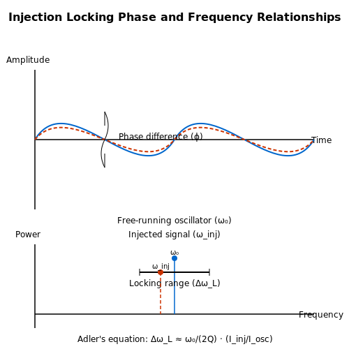
An injection-locked oscillator (ILO) synchronizes its output frequency and phase to an external injected signal when the injected signal's frequency lies within a finite range around the oscillator's natural frequency. This phenomenon, known as injection locking, arises due to nonlinear interactions between the oscillator's intrinsic dynamics and the external forcing signal.
Mathematical Derivation of Locking Range
The locking range ΔωL defines the maximum frequency deviation between the injected signal (ωinj) and the free-running oscillator frequency (ω0) for which locking can occur. For a weakly nonlinear oscillator, Adler's equation describes the phase dynamics:
where ϕ is the phase difference between the oscillator and injected signal, Δω = ωinj - ω0, and ωL is the locking range parameter. The steady-state solution requires dϕ/dt = 0, leading to:
The locking condition is satisfied when |Δω| ≤ ωL, defining the maximum locking range. For a typical LC oscillator, the locking range relates to the quality factor Q and injection strength α:
Mechanisms of Injection Locking
Injection locking occurs through two primary mechanisms in oscillators:
- Nonlinear phase correction: The oscillator's amplitude-limiting nonlinearity converts injected signal phase variations into frequency corrections.
- Regenerative amplification: The injected signal experiences gain at frequencies near resonance, reinforcing synchronization.
These mechanisms create a stable equilibrium where the oscillator's phase continuously adjusts to match the injected signal, provided the frequency difference remains within the locking range.
Practical Considerations
Key parameters affecting injection locking performance include:
- Injection ratio: Defined as the power ratio between injected signal and oscillator output, typically ranging from -30 dB to -10 dB for effective locking.
- Quality factor: Lower-Q oscillators exhibit wider locking ranges but poorer phase noise performance.
- Injection point: Optimal coupling depends on oscillator topology (e.g., Colpitts, Hartley, or ring oscillators).
Modern applications leverage injection locking in phase-locked loops, clock distribution networks, and high-efficiency RF power amplifiers, where precise frequency control and low phase noise are critical.
Nonlinear Dynamics Perspective
From a nonlinear systems viewpoint, injection locking represents a synchronization of coupled oscillators. The Van der Pol oscillator model provides insight into this behavior:
where ϵ governs the nonlinear damping and F is the injection amplitude. Numerical analysis of this equation reveals Arnold tongues - regions in parameter space where locking occurs.
1.2 Key Parameters Affecting Locking Range
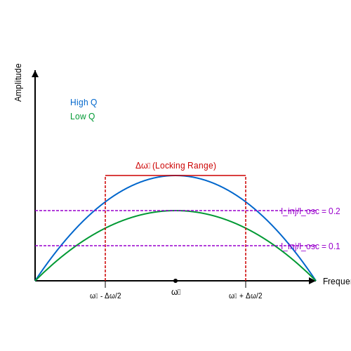
The locking range of an injection-locked oscillator (ILO) defines the frequency range over which the oscillator can synchronize with an external injected signal. Several critical parameters influence this range, including the quality factor (Q), injection strength, nonlinearity of the active device, and frequency detuning.
Quality Factor (Q) and Resonator Bandwidth
The quality factor of the resonator directly impacts the locking range. A lower Q results in a wider locking range due to the broader bandwidth of the resonator. The relationship can be derived from Adler's equation for injection locking:
where:
- ΔωL is the locking range in radians per second,
- ω0 is the free-running oscillator frequency,
- Q is the quality factor of the resonator,
- Iinj is the injected current amplitude,
- Iosc is the oscillator's sustaining current.
This equation shows that reducing Q or increasing the injection ratio (Iinj/Iosc) widens the locking range.
Injection Strength and Nonlinearity
The injection strength, defined as the ratio of injected power to the oscillator's output power, plays a crucial role. A stronger injection signal forces the oscillator to lock over a broader frequency range. However, the nonlinearity of the active device (e.g., a transistor) introduces saturation effects, limiting the maximum achievable locking range. The locking range can be approximated for weakly nonlinear systems as:
where Pinj and Posc are the injected and oscillator power levels, respectively.
Frequency Detuning and Phase Noise
Frequency detuning (Δω = ωinj − ω0) affects the locking range, with larger detuning requiring higher injection power to maintain lock. Phase noise also plays a role—higher phase noise in the free-running oscillator reduces the effective locking range due to increased jitter.
Practical Implications in RF Design
In RF and microwave applications, optimizing the locking range involves:
- Choosing resonators with an appropriate Q (e.g., LC tanks for wider locking ranges, crystal oscillators for narrow ranges).
- Balancing injection power to avoid excessive nonlinear distortion.
- Minimizing phase noise through proper biasing and low-noise active devices.
For example, in phased-array systems, a wide locking range allows for flexible frequency synchronization across multiple ILOs, while in clock recovery circuits, a narrower range may be preferred for noise immunity.
Comparison with Free-Running Oscillators
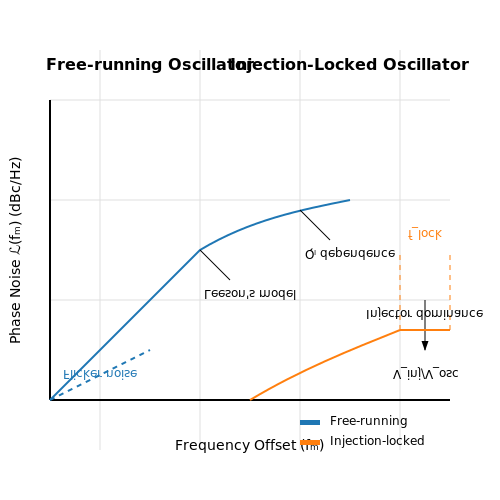
Injection-locked oscillators (ILOs) exhibit fundamentally different behavior compared to free-running oscillators due to the presence of an external synchronization signal. The key distinctions arise in phase noise, frequency stability, and spectral purity, which are critical in applications such as frequency synthesis, clock recovery, and coherent communication systems.
Phase Noise and Spectral Purity
Free-running oscillators rely solely on their resonant tank circuit for frequency determination, leading to phase noise that follows Leeson's model:
where F is the noise factor, QL is the loaded quality factor, and fc is the flicker noise corner frequency. In contrast, an ILO phase noise is dominated by the injected signal within its lock range, suppressing the oscillator's intrinsic noise. The resulting phase noise ℒILO(fm) approximates:
where flock is the locking bandwidth and ℒinj is the injector's phase noise. This makes ILOs superior in low-phase-noise applications like millimeter-wave transceivers.
Frequency Stability and Locking Range
Free-running oscillators are sensitive to environmental perturbations (temperature, supply voltage), causing frequency drift. The fractional frequency stability is given by:
where α, β, and γ are coefficients for thermal, voltage, and aging effects. An ILO, however, tracks the injector's frequency within the Adlerian lock range:
where Vinj/Vosc is the injection ratio. Beyond this range, the oscillator reverts to free-running behavior with abrupt phase slips.
Nonlinear Dynamics and Pulling Effects
Free-running oscillators operate in a limit-cycle regime, describable by the van der Pol equation:
ILOs, however, exhibit forced synchronization, modeled as a perturbed nonlinear system:
This leads to hysteresis and bifurcation phenomena near the lock boundaries, which are exploited in injection-pulling compensation techniques for RFICs.
Practical Trade-offs
- Design Complexity: ILOs require precise injector coupling and stability, while free-running oscillators need high-Q resonators.
- Power Consumption: ILOs often consume less power than PLL-based synthesizers but more than standalone LC oscillators.
- Jitter Accumulation: Free-running oscillators suffer from unbounded jitter, whereas ILOs inherit the injector's jitter characteristics.
Modern applications leverage hybrid approaches, such as self-injection locking in optoelectronic oscillators, to combine the benefits of both architectures.
2. Voltage-Controlled Oscillators (VCOs) in Injection Locking
Voltage-Controlled Oscillators (VCOs) in Injection Locking
Fundamentals of VCO Operation
A Voltage-Controlled Oscillator (VCO) generates a periodic signal whose frequency is controlled by an input voltage. The output frequency fout is typically given by:
where f0 is the free-running frequency, KVCO is the tuning sensitivity (Hz/V), and Vctrl is the control voltage. In LC-tank VCOs, the frequency is adjusted by varying the capacitance of a varactor diode, while ring oscillators rely on delay modulation.
Injection Locking in VCOs
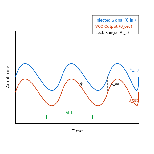
When an external signal is injected into a VCO, the oscillator may synchronize (lock) to the injected signal if the frequency difference falls within the lock range ΔfL. The lock range is derived from Adler's equation:
Here, Q is the tank quality factor, while Ainj and Aosc are the amplitudes of the injected and oscillator signals, respectively. Higher Q reduces the lock range, making the oscillator more selective but harder to lock.
Phase-Locking Dynamics
Under injection locking, the VCO's phase θosc aligns with the injected signal's phase θinj. The phase error ϕ = θinj - θosc follows a nonlinear differential equation:
where Δω is the initial frequency offset and ωL = 2πΔfL. The solution shows that the phase error converges to a steady-state value ϕss = sin-1(Δω/ωL) when locking occurs.
Practical Design Considerations
Injection-locked VCOs are widely used in:
- Frequency synthesizers for reduced phase noise.
- Clock recovery circuits where the VCO locks to an incoming data stream.
- Millimeter-wave systems to overcome limitations of standalone oscillators.
Key trade-offs include:
- Wider lock ranges require higher injection power, degrading phase noise.
- Lower KVCO improves stability but reduces tuning agility.
- Varactor nonlinearities introduce harmonic distortion.
Mathematical Analysis of Locking Bandwidth
The locking bandwidth BL can be derived from the open-loop transfer function of the injection-locked PLL. For a second-order system:
where ζ is the damping factor. This shows that increasing injection amplitude or KVCO widens the locking bandwidth, while higher oscillator amplitude narrows it.
2.2 LC and Ring Oscillator Implementations
LC Oscillator Topologies for Injection Locking
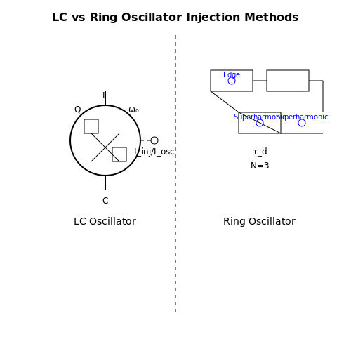
LC oscillators leverage resonant tanks to achieve high spectral purity, making them ideal for injection locking in RF applications. The locking range ΔωL is derived from Adler's equation:
where ω0 is the free-running frequency, Q is the tank quality factor, and Iinj/Iosc is the injection current ratio. Cross-coupled differential pairs (e.g., NMOS/PMOS) are commonly used for negative resistance generation, with injection applied via:
- Direct current injection at the tail node, modulating the bias current.
- Capacitive coupling to one of the tank nodes, perturbing the phase.
Ring Oscillator Implementations
Ring oscillators, composed of an odd number of inverter stages, offer wider locking ranges due to their inherent delay-based operation. The locking range scales with stage delay τd:
where N is the number of stages. Injection is typically applied by:
- Superharmonic locking at a multiple of the fundamental frequency.
- Edge injection, where the external signal overrides the internal delay mechanism.
Phase Noise Considerations
LC oscillators exhibit superior phase noise performance (∝ 1/Q²), while ring oscillators trade off noise for tunability. Injection locking reduces phase noise within the locking range by synchronizing to a cleaner reference.
Practical Trade-offs
| Parameter | LC Oscillator | Ring Oscillator |
|---|---|---|
| Locking Range | Narrow (~1-5%) | Wide (~10-50%) |
| Phase Noise | -120 to -160 dBc/Hz | -80 to -120 dBc/Hz |
| Power Consumption | High (tank Q) | Low (digital-like) |
Injection Locking in Microwave and mm-Wave Oscillators
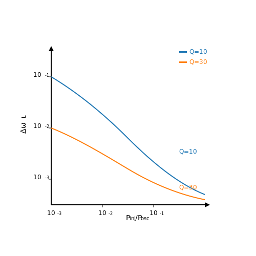
Injection locking in microwave and mm-wave oscillators is governed by Adler's equation, which describes the phase dynamics of an oscillator under external injection. The locking range ΔωL is derived from the nonlinear interaction between the injected signal and the oscillator's natural frequency. For a given injection power Pinj and oscillator output power Posc, the locking range is:
where ω0 is the free-running frequency and Q is the quality factor of the resonator. The locking range scales inversely with Q, making high-Q oscillators more resistant to injection locking but also more stable when locked.
Phase Noise Reduction Mechanism
Injection locking suppresses phase noise by forcing the oscillator to track the phase of the injected signal. The phase noise L(f) of the locked oscillator follows:
where Linj(f) and Losc(f) are the phase noise of the injected signal and free-running oscillator, respectively, and fL is the locking bandwidth. This behavior is exploited in mm-wave synthesizers to clean up noisy sources.
Nonlinear Effects and Stability
At mm-wave frequencies (>30 GHz), nonlinearities in active devices (e.g., HBTs or HEMTs) introduce additional complexity. The locking range becomes asymmetric due to:
- Harmonic injection: Subharmonic locking via parametric excitation of nonlinear capacitances.
- AM-to-PM conversion: Amplitude fluctuations modulating the oscillator's phase delay.
The stability criterion for a locked oscillator requires the injection strength to satisfy:
where Δω is the initial frequency offset. Violating this condition leads to cycle slipping or chaotic behavior.
Implementation in mm-Wave Systems
Practical implementations use:
- Coupled oscillators: Arrays of injection-locked oscillators for power combining at 60–100 GHz.
- Subharmonic injection: Lower-frequency reference signals multiplied via harmonic locking.
- Optical injection: In photonic-mm-wave systems, where lasers modulate high-speed photodiodes.
A 94-GHz oscillator locked to a 10-MHz reference demonstrates phase noise reduction from −80 dBc/Hz to −110 dBc/Hz at 100-kHz offset, with locking bandwidth of 15 MHz for Q ≈ 20.
3. Phase-Locked Loop (PLL) Analogies
3.1 Phase-Locked Loop (PLL) Analogies
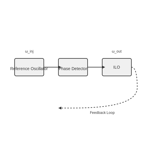
Injection-locked oscillators (ILOs) share fundamental operational principles with phase-locked loops (PLLs), particularly in their phase synchronization mechanisms. Both systems rely on feedback control to align the phase of an output signal with a reference input, though their implementations differ in topology and application constraints.
Phase Detector Equivalence
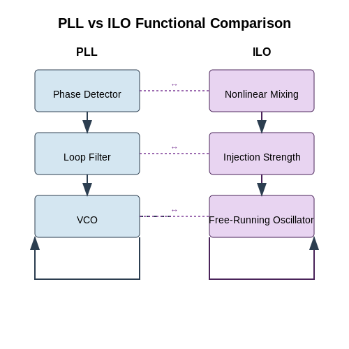
The phase detector in a PLL performs a similar function to the nonlinear mixing process in an ILO. In a PLL, the phase detector generates an error voltage proportional to the phase difference between the reference and feedback signals:
where Kpd is the phase detector gain. In an ILO, the injection signal mixes with the oscillator's natural output through device nonlinearities, producing an equivalent phase correction effect. The locking range ΔωL of an ILO mirrors the hold-in range of a PLL, both representing the maximum frequency deviation where synchronization can be maintained.
Loop Filter and Injection Strength
The PLL's loop filter finds its counterpart in the injection strength parameter of an ILO. A second-order PLL with a proportional-integral (PI) filter:
has direct analogy to the damping factor in an ILO, controlled by the injection ratio γ = Iinj/Iosc. Higher injection ratios correspond to wider locking ranges, similar to how higher loop filter bandwidths increase PLL acquisition range.
Voltage-Controlled Oscillator vs. Free-Running Oscillator
The VCO in a PLL adjusts frequency based on a control voltage, while an ILO's frequency is pulled by the injected signal. The ILO's phase dynamics follow Adler's equation:
where ωL is the locking range. This mirrors the PLL's phase dynamics equation when the VCO control sensitivity Kvco is replaced by the injection locking gain.
Stability Considerations
Both systems exhibit similar stability criteria. A PLL's phase margin requirement translates to the ILO's maximum tolerable phase perturbation before losing lock. The ILO's quality factor Q affects its phase noise performance and locking range, analogous to how PLL bandwidth trades off between noise suppression and settling time.
Practical Implementation Tradeoffs
While PLLs offer precise digital control through frequency dividers, ILOs provide superior high-frequency performance with simpler architectures. Modern systems often combine both approaches, using ILOs for millimeter-wave generation while employing PLLs for lower-frequency reference synthesis.
3.2 Nonlinear Dynamics and Stability Criteria
The behavior of injection-locked oscillators (ILOs) is governed by nonlinear dynamics, where the interaction between the injected signal and the oscillator's intrinsic nonlinearities determines the locking range and stability. The Adler equation provides a fundamental framework for analyzing this behavior, but deeper insights require examining the phase-space dynamics and stability boundaries.
Phase Dynamics and the Adler Equation
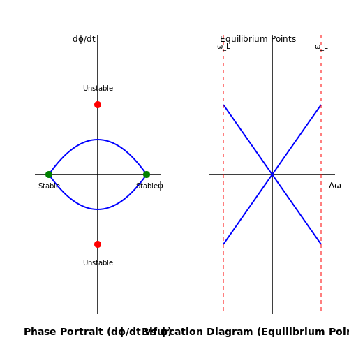
The phase difference ϕ between the injected signal and the oscillator output evolves according to the Adler equation:
where Δω is the detuning frequency (ωinj - ω0) and ωL is the locking range. The equilibrium points occur when dϕ/dt = 0, leading to:
This equation implies that locking is only possible when |Δω| ≤ ωL, defining the fundamental locking range.
Stability Analysis
To assess stability, we linearize the system around equilibrium points. Consider small perturbations δϕ about an equilibrium phase ϕ0:
The perturbation dynamics are governed by the eigenvalue λ = -ωLcosϕ0. Stability requires Re(λ) < 0, which occurs when:
This condition defines the stable branch of solutions. The unstable equilibrium occurs when cosϕ0 < 0, corresponding to the top half of the sine characteristic where small perturbations grow exponentially.
Nonlinear Effects and Higher-Order Dynamics
When the injection strength increases beyond weak coupling, higher-order nonlinearities become significant. The generalized phase equation incorporates these effects:
where ϵ represents the strength of second-harmonic nonlinearities. This creates additional equilibrium points and can lead to bifurcations in the phase portrait. The stability criteria now involve evaluating the Jacobian matrix of the nonlinear system.
Practical Stability Considerations
In real implementations, several factors affect stability:
- Phase noise: Contributes stochastic perturbations that may drive the system out of lock
- Parameter variations: Temperature and supply voltage changes modify ωL and Δω
- Nonlinear saturation: Limits the maximum achievable locking range
Engineers often use phase margin analysis to ensure robust operation. The phase margin is defined as the angular distance from the unstable equilibrium:
A practical design rule maintains ϕm ≥ 45° across the expected parameter variations.
Bifurcation Analysis
As injection parameters vary, the system may undergo bifurcations - qualitative changes in dynamic behavior. The most common in ILOs are:
- Saddle-node bifurcation: Occurs at the locking range boundary when stable and unstable equilibria collide
- Hopf bifurcation: Can lead to the emergence of limit cycles outside the locking range
The bifurcation diagram reveals how the number and stability of equilibrium points change with detuning. This analysis is crucial for designing injection-locked PLLs and frequency synthesizers where parameter drift must not cause sudden loss of lock.
Multistability and Hysteresis
In strongly nonlinear regimes, ILOs can exhibit multistable regions where multiple stable equilibrium points coexist. This leads to hysteresis effects where the locking behavior depends on the direction of frequency sweep. The hysteresis width Δωh is given by:
when ϵ < 2ωL. This effect is exploited in certain memory applications and bistable frequency converters.
3.3 Adler's Equation and Its Applications
Adler's equation provides a fundamental framework for analyzing the phase dynamics of an injection-locked oscillator. It describes how an external signal influences the oscillator's phase, leading to synchronization when certain conditions are met. The derivation begins with the nonlinear differential equation governing the phase difference ϕ(t) between the injected signal and the oscillator's natural output.
Derivation of Adler's Equation
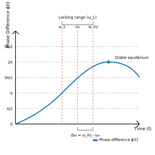
Consider an oscillator with a free-running frequency ω₀ subjected to an injected signal of frequency ωinj and amplitude Vinj. The phase error ϕ(t) evolves according to:
where Δω = ω₀ - ωinj is the detuning frequency, and ωL is the locking range given by:
Here, Q is the quality factor of the oscillator, and Vosc is the oscillator's output amplitude. The term ωL sin(ϕ) represents the restoring force that pulls the oscillator phase toward synchronization.
Locking Range and Stability Analysis
The locking condition occurs when dϕ/dt = 0, leading to:
For synchronization to be possible, the detuning must satisfy |Δω| ≤ ωL. Beyond this range, the oscillator fails to lock, resulting in periodic phase slips. The steady-state phase error ϕss is given by:
Stability analysis via linearization around ϕss reveals that the equilibrium point is stable when cos(ϕss) > 0, ensuring phase-locking.
Applications in Modern Systems
Adler's equation underpins several critical applications:
- Frequency Synthesizers: Injection locking enables low-phase-noise frequency generation by locking a voltage-controlled oscillator (VCO) to a stable reference.
- Phase-Locked Loops (PLLs): The dynamics described by Adler's equation are analogous to PLL behavior, aiding in loop bandwidth optimization.
- Wireless Receivers: Injection-locked oscillators serve as high-sensitivity demodulators in coherent receivers by tracking the phase of incoming signals.
Nonlinear Extensions and Practical Considerations
While Adler's equation assumes weak injection, practical systems often require extensions for strong injection regimes. Modified versions incorporate higher-order nonlinearities, such as:
where ϵ accounts for harmonic effects. Experimental validation in RF systems shows close agreement with theoretical predictions when parasitic effects (e.g., tank circuit losses) are minimized.
4. Frequency Synthesis and Clock Recovery
4.1 Frequency Synthesis and Clock Recovery
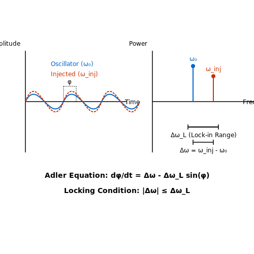
Injection-locked oscillators (ILOs) are widely employed in frequency synthesis and clock recovery due to their ability to synchronize with an external reference signal while maintaining low phase noise. The locking phenomenon occurs when an oscillator's free-running frequency (ω0) is perturbed by an injected signal (ωinj), forcing it to lock within a finite range known as the lock-in range (ΔωL).
Locking Condition and Phase Dynamics
The Adler equation governs the phase dynamics of an ILO under injection:
where Δω = ωinj − ω0 is the initial frequency detuning, ωL is the locking range, and ϕ is the phase difference between the injected and oscillator signals. For stable locking, the condition |Δω| ≤ ωL must be satisfied. The locking range is derived as:
where Q is the quality factor of the oscillator, and Iinj/Iosc is the injection strength ratio.
Frequency Synthesis via Harmonic Locking
ILOs enable frequency multiplication by locking to harmonics of the reference signal. If the oscillator is designed to operate at nωinj, the output frequency becomes:
This principle is exploited in sub-harmonically injection-locked PLLs (SHIL-PLLs), where a lower-frequency reference locks a higher-frequency VCO, reducing phase noise compared to traditional charge-pump PLLs.
Clock Recovery in Communication Systems
In clock and data recovery (CDR) circuits, ILOs extract timing information from noisy data streams. The oscillator locks to the embedded clock component of the input signal, rejecting jitter outside its bandwidth. The key metrics are:
- Jitter tolerance: Maximum input jitter without losing lock.
- Lock time: Duration to achieve phase alignment after initial detuning.
A typical implementation uses a Bang-Bang phase detector to adjust the injection strength dynamically, optimizing the trade-off between lock range and phase noise.
Practical Considerations
Nonlinearities in the oscillator's active devices introduce pulling effects, where the locked frequency deviates from the ideal linear relationship. This is modeled by:
where Kp is the pulling coefficient. Advanced designs employ differential oscillators or harmonic rejection techniques to mitigate this issue.
4.2 Phase Noise Reduction Techniques
Fundamentals of Phase Noise in Injection Locked Oscillators
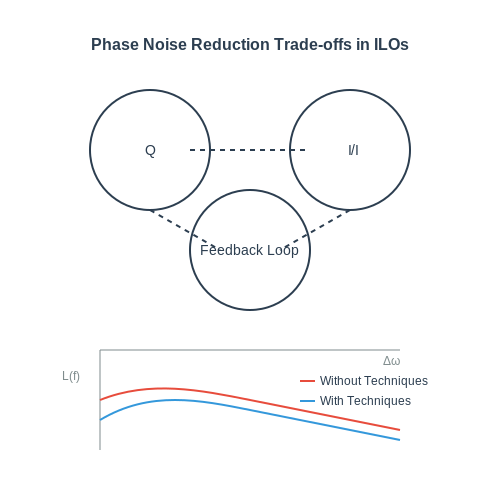
Phase noise in injection-locked oscillators (ILOs) arises from intrinsic noise sources such as thermal noise, flicker noise, and shot noise, which perturb the oscillator's timing jitter. The phase noise spectrum \( \mathcal{L}(f) \) is typically modeled using Leeson's equation, modified for ILOs:
where \( F \) is the noise figure, \( Q_L \) is the loaded quality factor, \( f_0 \) is the carrier frequency, and \( f_c \) is the flicker noise corner frequency. Injection locking suppresses phase noise by forcing the oscillator to track the cleaner reference signal, but residual noise persists due to imperfect locking bandwidth and nonlinearities.
Key Techniques for Phase Noise Reduction
1. Optimizing Injection Power and Locking Bandwidth
The locking range \( \Delta \omega_L \) of an ILO is given by:
where \( I_{inj} \) and \( I_{osc} \) are the injection and oscillator currents, respectively. Increasing \( I_{inj} \) widens the locking range but risks introducing spurious tones. Empirical studies show a trade-off: phase noise reduction plateaus when \( I_{inj}/I_{osc} > 0.1 \), while excessive injection power degrades spectral purity.
2. High-Q Resonator Design
The loaded quality factor \( Q_L \) directly impacts phase noise:
Techniques include:
- Superconducting resonators (e.g., NbTiN) achieving \( Q > 10^6 \) at cryogenic temperatures.
- MEMS-based tanks with \( Q \sim 10^4 \) in integrated designs.
- Dielectric-filled cavities for millimeter-wave applications.
3. Subharmonic Injection Locking
Locking to a subharmonic (e.g., \( f_{ref} = f_0/N \)) reduces reference oscillator phase noise by \( 20 \log N \). The phase transfer function becomes:
where \( \omega_L \) is the loop bandwidth. This technique is prevalent in optical comb generation and THz frequency synthesis.
Advanced Active Noise Cancellation
Feedforward and feedback methods actively correct phase errors:
- Feedforward: A secondary path injects an anti-phase noise signal, canceling perturbations. Demonstrated in 5G mmWave ILOs with 8 dB phase noise improvement.
- Feedback: A PLL-like loop filters residual noise. The challenge lies in avoiding instability when combined with injection locking.
Case Study: Low-Noise ILO for Quantum Computing
In a 2022 implementation, a 10 GHz ILO using a sapphire-loaded cavity (\( Q = 50,000 \)) and optimized injection ratio achieved \( \mathcal{L}(-100 \text{ dBc/Hz at 1 kHz offset}) \). Key innovations included:
- Subharmonic locking to a 100 MHz ultra-low-noise quartz reference.
- Active noise cancellation via a superconducting quantum interference device (SQUID) array.
Nonlinear Phase Noise Compression
In strongly nonlinear ILOs (e.g., CMOS ring oscillators), phase noise compression occurs when:
where \( \alpha \) is the nonlinearity coefficient and \( \Gamma(t) \) represents noise. Third-order nonlinearities can suppress close-in phase noise by 3–5 dB, as validated in recent silicon photonics experiments.
4.3 Injection Locking in Wireless Communication Systems
Injection locking plays a critical role in modern wireless communication systems, particularly in frequency synchronization, phase noise reduction, and coherent signal reception. When an external signal is injected into an oscillator, the oscillator's frequency and phase align with the injected signal within a finite locking range. This phenomenon is exploited in various wireless applications, from local oscillators (LOs) in transceivers to carrier recovery in demodulators.
Mathematical Basis of Injection Locking
The locking range ΔωL of an injection-locked oscillator (ILO) is derived from Adler's equation, which describes the phase dynamics of the system:
Here, ω0 is the free-running frequency, ωinj is the injected signal frequency, Q is the quality factor, and Ainj/A0 is the injection strength ratio. The locking range is obtained when the phase derivative dφ/dt stabilizes to zero:
This shows that the locking range is inversely proportional to Q and directly proportional to the injection strength.
Applications in Wireless Systems
1. Frequency Synthesizers
Injection-locked frequency dividers (ILFDs) are widely used in phase-locked loops (PLLs) for high-frequency synthesis. By locking a voltage-controlled oscillator (VCO) to a subharmonic of a reference signal, ILFDs enable low-phase-noise frequency generation with reduced power consumption compared to traditional dividers.
2. Carrier Recovery
In coherent receivers, injection locking aids in carrier synchronization by forcing the local oscillator to track the phase of the incoming modulated signal. This is particularly useful in high-order modulation schemes (e.g., QAM) where phase noise can degrade the error vector magnitude (EVM).
3. Beamforming and MIMO Systems
In phased-array antennas, injection locking ensures phase coherence across multiple oscillators, enabling precise beam steering. For massive MIMO systems, this technique reduces calibration overhead by synchronizing distributed LO signals.
Practical Considerations
- Injection Power Sensitivity: The locking range is highly dependent on the injected signal power. Too little power results in insufficient locking, while excessive power can distort the oscillator's output.
- Phase Noise Suppression: Injection locking reduces phase noise within the locking bandwidth, but out-of-band noise may remain unaffected.
- Stability Trade-offs: High-Q oscillators offer narrow locking ranges but better noise performance, whereas low-Q oscillators lock more easily but exhibit higher phase noise.
Case Study: Injection-Locked PLL for 5G mmWave
A recent implementation for 28 GHz 5G transceivers demonstrated a 40% reduction in power consumption by replacing a conventional fractional-N PLL with an injection-locked architecture. The ILO achieved a phase noise of −110 dBc/Hz at 1 MHz offset while maintaining a locking range of ±150 MHz.
5. Key Research Papers and Books
5.1 Key Research Papers and Books
- PDF 1-GHz and 2.8-GHz CMOS Injection-locked Ring Oscillator Prescalers — by exploiting the injection locking phenomena in differential CMOS ring oscillators. We tested a 5-stage, 1-GHz injection-locked modulo-8 prescaler fabricated in a 0.24-µm CMOS technology that consumes 350 µW of power and occupies 0.012 mm2 of die area. The locking range is 20 MHz and the locked phase noise is -110 dBc/Hz @ 100 kHz. A 2.8-GHz, 3-
- Injection locked oscillator arrays for spectrum analysis — Injection locked oscillator arrays are described as a means of quasi-real-time spectrum analysis. Two oscillators with closely spaced frequencies at 5.1 and 5.8 GHz were designed such that single or simultaneous injection locking may occur depending on the injected frequency and power. The locking range for a -20 dBm input is greater than 150 MHz for each oscillator and at 0 dBm the ...
- PDF Topics in IC Design 4.1 Introduction to Injection Locked Oscillators — Amplitude when Injection Locked • When the oscillator is injection locked with , oscillation frequency becomes injection frequency s. • In steady state, and right hand side is . • Since , Topics in IC Design 14 Result of injection on amplitude: Phase difference between
- PDF Injection-Locked Ring Oscillators - research.asu.edu.eg — This thesis discusses the analysis and the design of an injection-locked ring oscillator for forward-clocking architecture in serial-link transceivers. The injection locking mechanism is analysed and employed in the super-harmonic injection locking scheme. In this scheme, super-harmonic injection is introduced to a ring oscillator
- Architectures and Circuits Leveraging Injection-Locked Oscillators for ... — 2-14 Injection lock transient waveforms for the di erential 4-stage ring os-cillator used for the derivation of Δ[ + 1] from Δ[ ]. . . . . . . . . .28 2-15 Simulated and calculated injection lock dynamics of the di erential 4-stage ring oscillator for a step change in frequency from 3.4MHz to
- PDF Injection Locked Clocking and Transmitter Equalization Techniques for ... — The inherent dynamics of injection locked quadrature ring oscillator are used to improve its locking range from 5% (7-7.4GHz) to 90% (4-11GHz). The QLL is used to generate accurate clock phases for a four channel optical receiver using a forwarded clock at quarter-rate. The QLL drives an injection locked oscillator (ILO) at each channel without any
- (PDF) Multiband multimode Injection-locked Oszillatoren mit Slow-Wave ... — The 1/f additive phase noise of one-port injection-locked oscillators is experimentally characterized and analyzed using a simple analytic model based on the generalized 1/f Kurokawa theory. To experimentally verify the prediction of the simple analytic model proposed, two negative-conductance transmission line pHEMT oscillators operating at 2. ...
- A study of Injection Locking in Optoelectronic Oscillator — lence inspired me throughout this research. This thesis would not have been possible without his support and nally would like to thank him once again for putting up with my questions and doubts. I thank profusely my colleagues from research group Mehedi Hasan and Minu Sunny who o ered kind help and co- operation during the research period. I
- Injection-Locking Techniques for Nonharmonic Oscillators — Assume that the frequency of the injection signal ω inj = ω o + Δω falls into the lock range of the oscillator such that the oscillator will be locked to the injection signal and will oscillate at ω inj once it is locked. The first-order Volterra circuit is linear with its inputs at ω inj.Its outputs therefore only contain frequency components at ω inj and can be written as
- A Fully Synthesized Injection Locked Ring Oscillator Based on a Pulse ... — Fig. 3.9 Pulse Injection Method in Time Domain ..... 47 Fig. 3.10 Active High Tristate Inverter with Output Buffer ..... 48 Fig. 3.11 Proposed Injection Locked Ring Oscillator of the High-Frequency Oscillator 49
5.2 Online Resources and Tutorials
- PDF A Wideband Injection Locking Scheme and Quadrature Phase Generation in ... — Index Terms — injection-locked oscillator, injection-locked phase-locked loop, locking range, quadrature, jitter transfer function, voltage-controlled oscillator (VCO). I. INTRODUCTION Injection-locked-oscillators (ILOs) have been used in many wireline receivers because of their simple implementation and instantaneous locking characteristics.
- Injection-Locking Techniques for Nonharmonic Oscillators — A comparison of (5.6) and (5.7) with (4.54) and (4.55) reveals that nonlinearity factor a affects the governing equations of both the first- and third-order Volterra circuits. For the first-order Volterra circuit, it changes the transconductance of the transconductors from J to aJ, as shown in Fig. 5.4.For the third-order Volterra circuit, its impact is three-fold: (a) It changes the ...
- Theory of Injection-Locked Oscillator Phase Noise - studylib.net — 312 IEEE TRANSACTIONS ON CIRCUITS AND SYSTEMS—I: REGULAR PAPERS, VOL. 58, NO. 2, FEBRUARY 2011 Theory of Injection-Locked Oscillator Phase Noise Torsten Djurhuus and Viktor Krozer, Senior Member, IEEE Abstract—The paper describes the development of a model for the calculation of noise-driven phase response of an injection-locked oscillator perturbed by Gaussian white sources.
- PDF Topics in IC Design 4.1 Introduction to Injection Locked Oscillators — Amplitude when Injection Locked • When the oscillator is injection locked with , oscillation frequency becomes injection frequency s. • In steady state, and right hand side is . • Since , Topics in IC Design 14 Result of injection on amplitude: Phase difference between
- DTIC ADA254892: Quartz Crystal Resonators and Oscillators for Frequency ... — Subjects covered include: applications of frequency standards; types of oscillators (quartz and atomic); quartz resonator properties; quartz growing, sweeping, and material characteristics; Q and its significance; resonator and oscillator stability, including aging, short-term instability, frequency vs. temperature characteristics, oscillator circuit caused instabilities, frequency vs. drive ...
- PDF Injection-Locked Ring Oscillators — Injection-Locked Ring Oscillators By Eman Salah El-Din Fahmy Ibrahim Master of Science in Electrical Engineering (Electronics and Electrical Communication Engineering) Examiners' Committee Name and Affiliation Signature Prof. Dr. Elsayed Mostafa Saad (Examiner) Electronics, Communications and Computer Engineering Dept.,
- (PDF) Radiation-Hardened 5.2 GHz ILO for RF Use - Academia.edu — In this paper, an 8GHz 16 th sub-harmonic Injection-Locked Oscillator based on LC-oscillators and pulse generators is presented. It has been fully implemented in a VLSI 65nm CMOS technology from STMicroelectronics and is dedicated to a double-loop frequency synthesizer.
- PDF Injection Locked Clocking and Transmitter Equalization Techniques for ... — The inherent dynamics of injection locked quadrature ring oscillator are used to improve its locking range from 5% (7-7.4GHz) to 90% (4-11GHz). The QLL is used to generate accurate clock phases for a four channel optical receiver using a forwarded clock at quarter-rate. The QLL drives an injection locked oscillator (ILO) at each channel without any
- Injection-Locked Oscillators - SpringerLink — 7.5.2.1 The Injection-Locked Receiver As mentioned earlier, the phase difference \(\phi _i\) between the injected signal and the oscillator is always between \({\pm }90^\circ \). However, by applying an abrupt phase step to the injected signal, the oscillator will instantaneously lose its lock condition.
- Injection-Locking of Harmonic Oscillators | SpringerLink — For injection-locked harmonic oscillators with a spiral inductor resonator, since the value of the components of the resonator does not vary with the injection signal, the variation of the impedance caused by the injection signal is solely due to the displacement of the frequency from ω o to ω o + Δω in order to satisfy Barkhausen criteria ...
5.3 Advanced Topics for Further Study
- PDF Injection-locked Ring Oscillator Frequency Dividers — INJECTION-LOCKED RING OSCILLATOR FREQUENCY DIVIDERS A THESIS ... ring oscillators. Injection locking—the synchronization in frequency and phase ... 5-3 Evolution of the injection-locked loop.....92 5-4 Phase contribution of the mixer.....93 5-5 Evolution of the injection-locked loop: phase contribution ...
- PDF Topics in IC Design 4.1 Introduction to Injection Locked Oscillators — Amplitude when Injection Locked • When the oscillator is injection locked with , oscillation frequency becomes injection frequency s. • In steady state, and right hand side is . • Since , Topics in IC Design 14 Result of injection on amplitude: Phase difference between
- A study of Injection Locking in Optoelectronic Oscillator — high-speed digital electronics, radar, and astronomy. The Optoelec-tronic Oscillator (OE Oscillator), a new class of time delay oscillator ... 1 Summary of research work on optoelectronic oscillators . . . .5 2 List of parameters used in OE Oscillator prototype simulation71 xii. ... MIL-OEOMutually Injection Locked Optoelectronic Oscillator ...
- PDF Locking Techniques for RF Oscillators at 5 - 6 GHz Frequency Range - uth.gr — called Injection Locked Phase Locked Loop (ILPLL). During recent years several researchers have been involved in the study of the ILPLL [1-5], which demonstrates superior noise performance, high output This work was supported by THETA S.A. (a fully owned subsidiary of Theta Microelectronics Inc.) power and wider locking bandwidth compared to the
- Injection Locking: Oscillators & Adler's Equation - studylib.net — The system is injection locked to a super-harmonic NJECTION-LOCKED OSCILLATORS II. free-running MODEL FOR Ifrequency.! of the An non-linearity LC oscillator in can modeled as a nonlinear block The thebeloop must create intermodulation products thatby falla infrequency the passband of the loop. , followed selective block (e.g., an RLC or ...
- Injection-Locking Techniques for Nonharmonic Oscillators — Assume that the frequency of the injection signal ω inj = ω o + Δω falls into the lock range of the oscillator such that the oscillator will be locked to the injection signal and will oscillate at ω inj once it is locked. The first-order Volterra circuit is linear with its inputs at ω inj.Its outputs therefore only contain frequency components at ω inj and can be written as
- A Fully Synthesized Injection Locked Ring Oscillator Based on a Pulse ... — Fig. 3.9 Pulse Injection Method in Time Domain ..... 47 Fig. 3.10 Active High Tristate Inverter with Output Buffer ..... 48 Fig. 3.11 Proposed Injection Locked Ring Oscillator of the High-Frequency Oscillator 49
- Design and optimization of the ring oscillator based injection locked ... — A ring-based injection-locked clock multiplier (ILCM) is implemented to show the effectiveness of the reference quadrupler. The output clock of ILCM achieves an integrated jitter of 387 fs rms at 2.8 GHz output frequency with a total multiplication factor of 56 and 6.2 mW consumed power from 1.2 V supply.
- Design of injection‐locked oscillator circuits using an HBT X ... — Injection-locked oscillators are circuits able to oscillate in the presence of an input periodic signal at the frequency ω in. Thus, the oscillation frequency ω o in free-running mode is influenced by the input signal and may take different ω a values: ω a / ω in = m / k, with m and k integer values.