Wireless Power Transfer Technologies
1. Principles of Inductive Coupling
Principles of Inductive Coupling
Fundamental Theory
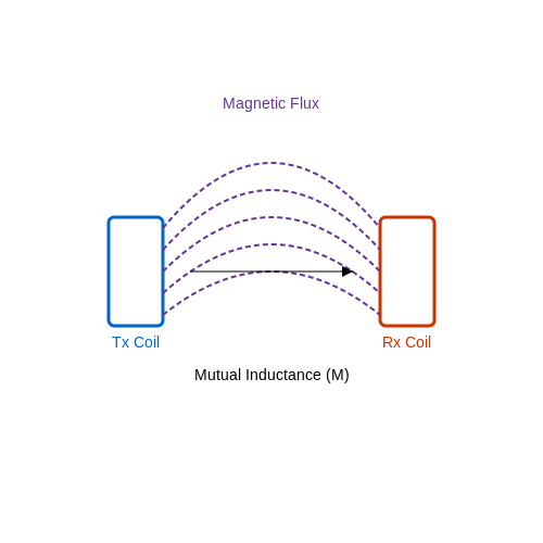
Inductive coupling operates on Faraday's Law of Electromagnetic Induction, where a time-varying magnetic field generated by a primary coil induces a voltage in a secondary coil. The mutual inductance M between two coils determines the efficiency of power transfer and is given by:
where k is the coupling coefficient (0 ≤ k ≤ 1), and L1, L2 are the self-inductances of the primary and secondary coils, respectively. For tightly coupled systems (k > 0.5), near-field energy transfer dominates, while loosely coupled systems (k < 0.3) suffer from significant leakage flux.
Resonant Inductive Coupling
To enhance efficiency in loosely coupled scenarios, resonant circuits are employed. The primary and secondary coils are tuned to the same resonant frequency fr:
where L is the coil inductance and C is the compensating capacitance. This technique, known as resonant inductive coupling (RIC), reduces reactive power losses and enables mid-range wireless power transfer (up to several meters).
Key Performance Metrics
The efficiency η of inductive power transfer is governed by:
where Q1 and Q2 are the quality factors of the primary and secondary circuits. High-Q coils (> 100) are essential for efficient energy transfer, particularly in biomedical implants or electric vehicle charging systems.
Practical Design Considerations
- Coil Geometry: Planar spiral coils offer better coupling for compact devices, while solenoid coils provide higher Q factors.
- Frequency Selection: Typical systems operate at 100 kHz - 10 MHz, balancing between coil losses (skin effect) and regulatory constraints.
- Shielding: Ferrite layers are often used to direct magnetic flux and reduce electromagnetic interference (EMI).
Real-World Applications
Inductive coupling is implemented in:
- Qi-standard smartphone charging (3-15 W)
- Electric vehicle charging (SAE J2954, up to 22 kW)
- Medical implant powering (e.g., pacemakers)
- Industrial automation (contactless power for robots)
Challenges and Limitations
Key challenges include:
where Rac accounts for frequency-dependent conductor losses. Misalignment tolerance remains a critical design constraint, with modern systems achieving ±15 mm lateral displacement for 90% efficiency retention.

1.2 Resonant Inductive Coupling
Resonant inductive coupling enhances traditional inductive power transfer by tuning the transmitter and receiver coils to the same resonant frequency. This technique significantly improves efficiency and range compared to non-resonant inductive methods, making it suitable for mid-range wireless power applications.
Fundamental Principles
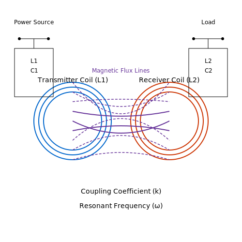
The system consists of two magnetically coupled LC circuits - a transmitter coil (L1) with capacitance (C1) and a receiver coil (L2) with capacitance (C2). Resonance occurs when:
where fr is the resonant frequency. Both circuits must be tuned to identical resonant frequencies for optimal power transfer.
Coupling Coefficient and Quality Factor
The coupling coefficient (k) describes the magnetic flux linkage between coils:
where M is the mutual inductance. The system's performance depends on both k and the quality factor (Q):
Higher Q factors enable stronger resonant effects but require tighter frequency matching.
Power Transfer Efficiency
The maximum efficiency (ηmax) occurs when:
This shows that efficiency depends on the product k2Q1Q2, known as the figure of merit.
Practical Implementation
Modern resonant systems typically operate in the 100 kHz to 10 MHz range. Key design considerations include:
- Coil geometry optimization for specific applications
- Precise frequency matching using variable capacitors or digital tuning
- Impedance matching networks to maximize power transfer
- Ferrite shielding to direct magnetic flux and reduce losses
Resonant inductive coupling enables wireless charging distances up to several times the coil diameter, with commercial systems achieving efficiencies exceeding 90% at optimal alignment.

Near-Field vs. Far-Field Energy Transfer
Fundamental Distinctions
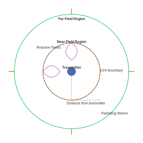
Wireless power transfer (WPT) systems are broadly categorized into near-field and far-field methods based on the distance relative to the transmitter's wavelength (λ). The near-field region, typically within a distance of λ/2π, is dominated by reactive fields (electric and magnetic), while the far-field region, beyond λ/2π, is characterized by propagating electromagnetic waves.
Near-Field Energy Transfer
Near-field WPT relies on non-radiative coupling, where energy is confined to the vicinity of the transmitter. The two primary mechanisms are:
- Inductive Coupling: Magnetic fields link transmitter and receiver coils, governed by Faraday's law of induction. The power transfer efficiency (η) depends on the coupling coefficient (k) and quality factors (Q) of the coils:
- Capacitive Coupling: Electric fields transfer energy between conductive plates. This method is less common but useful for low-power applications.
Far-Field Energy Transfer
Far-field WPT employs radiative electromagnetic waves (e.g., microwaves or lasers) for long-distance transmission. The power density (S) at distance d follows the inverse-square law:
where Pt is transmitted power and Gt is transmitter gain. Rectennas (rectifying antennas) are often used for RF-to-DC conversion.
Practical Implications
Near-field systems (e.g., Qi charging) excel in short-range, high-efficiency scenarios (e.g., >90% at cm-scale distances). Far-field systems (e.g., satellite solar power) enable long-range transfer but suffer from lower efficiency due to free-space path loss and atmospheric absorption.
Historical Context
Nikola Tesla's early experiments (1890s) with inductive coupling laid the groundwork for near-field WPT, while far-field concepts emerged later with microwave technology (1960s, e.g., William C. Brown's rectenna demonstrations).
2. Magnetic Resonance Coupling
2.1 Magnetic Resonance Coupling
Magnetic resonance coupling (MRC) is a highly efficient method of wireless power transfer that relies on the resonant interaction between two magnetically coupled coils. Unlike inductive coupling, MRC operates at a specific resonant frequency, enabling mid-range power transfer with reduced sensitivity to misalignment and distance variations.
Fundamental Principles
The efficiency of MRC is governed by the quality factor (Q) and the coupling coefficient (k) between the transmitter and receiver coils. The system consists of two LC resonators tuned to the same frequency, ensuring maximum energy transfer when:
where ω is the angular frequency, L is the inductance, and C is the capacitance of the resonant circuit. The coupling coefficient k is defined as:
where M is the mutual inductance, and L1, L2 are the inductances of the primary and secondary coils, respectively.
Power Transfer Efficiency
The efficiency (η) of MRC-based power transfer is derived from the coupled-mode theory and can be approximated as:
where Q1 and Q2 are the quality factors of the transmitter and receiver coils. High Q factors and strong coupling (k) lead to improved efficiency, but practical systems must balance these parameters to avoid bandwidth narrowing.
Practical Implementation
MRC systems typically operate in the frequency range of kHz to MHz, with common applications including:
- Electric vehicle charging – Enables wireless charging pads with higher tolerance to positioning errors.
- Medical implants – Powers devices without direct electrical contact, reducing infection risks.
- Consumer electronics – Supports wireless charging over distances of several centimeters.
Challenges and Optimization
Key challenges in MRC include:
- Frequency splitting – Occurs when coupling is too strong, leading to multiple resonant peaks.
- Loss mechanisms – Eddy currents and radiative losses reduce efficiency at higher frequencies.
- Regulatory constraints – Compliance with electromagnetic interference (EMI) standards is critical.
Optimization techniques involve adaptive impedance matching, frequency tuning, and the use of high-permeability materials to enhance magnetic flux confinement.
Radio Frequency (RF) Energy Harvesting
Fundamentals of RF Energy Harvesting
RF energy harvesting converts ambient electromagnetic waves into usable DC power through rectification. The process involves three primary stages: antenna reception, impedance matching, and rectification. The Friis transmission equation governs the power received by an antenna at distance d from a transmitter:
where Pr is received power, Pt is transmitted power, Gt and Gr are antenna gains, and λ is wavelength. Practical systems often operate in the μW to mW range due to path loss.
Rectenna Design
A rectifying antenna (rectenna) consists of:
- Antenna: Optimized for target frequencies (e.g., 900 MHz, 2.4 GHz).
- Matching network: Maximizes power transfer using conjugate matching.
- Schottky diode: Low-barrier diodes (e.g., HSMS-2850) minimize threshold voltage losses.
The rectifier's efficiency η is derived from:
where RL is load resistance and Vout is DC output voltage.
Multi-Band and Wideband Harvesting
Advanced designs employ:
- Dual-band antennas: Capture multiple ISM bands (e.g., 868 MHz + 2.4 GHz).
- Adaptive matching: Tunable LC networks compensate for impedance shifts.
- Voltage multipliers: Cockcroft-Walton cascades boost output at low input power.
Practical Challenges
Key limitations include:
- Low power density: Ambient RF fields rarely exceed 1 μW/cm².
- Nonlinear diode behavior: Harmonic generation reduces efficiency below -20 dBm.
- Regulatory constraints: FCC Part 15 limits unintentional radiation.
Applications
Notable implementations:
- Sensor networks: Battery-free IoT nodes using 915 MHz backscatter.
- Medical implants: Pacemakers powered by 402 MHz MICS band.
- RFID: Passive UHF tags (860–960 MHz) with integrated rectifiers.

2.3 Laser-Based Power Transfer
Laser-based power transfer (LBPT) utilizes coherent, monochromatic light to transmit energy wirelessly over long distances with minimal divergence. Unlike inductive or capacitive coupling, LBPT enables highly directional energy transmission, making it suitable for applications requiring precision, such as powering drones, satellites, or remote sensors.
Fundamentals of Laser Power Transmission
The efficiency of LBPT is governed by the Beer-Lambert law, which describes the attenuation of light as it propagates through a medium. The transmitted power \( P_t \) at a distance \( d \) is given by:
where \( P_0 \) is the initial laser power and \( \alpha \) is the attenuation coefficient of the medium. For vacuum or low-loss environments, \( \alpha \) approaches zero, enabling efficient long-range transmission.
Photovoltaic Receiver Design
The receiver typically consists of a high-efficiency photovoltaic (PV) cell optimized for the laser's wavelength. The power conversion efficiency \( \eta \) depends on the spectral match between the laser and the PV bandgap. For a monochromatic source, the theoretical maximum efficiency is given by:
where \( q \) is the electron charge, \( V_{oc} \) is the open-circuit voltage, \( FF \) is the fill factor, and \( E_{photon} \) is the photon energy. Advanced multi-junction cells can achieve efficiencies exceeding 50% under concentrated laser illumination.
Beam Shaping and Tracking
Precise beam control is critical to minimize losses. Adaptive optics and fast-steering mirrors compensate for atmospheric turbulence, while closed-loop tracking systems maintain alignment between the transmitter and receiver. The pointing error \( \theta \) must satisfy:
where \( \lambda \) is the wavelength and \( D \) is the aperture diameter. For a 1 µm laser and 10 cm aperture, the allowable error is below 10 µrad.
Safety and Thermal Management
High-power lasers pose eye and skin hazards, necessitating strict safety protocols. Systems often operate at eye-safe wavelengths (e.g., 1550 nm) or incorporate beam-shuttering mechanisms. Thermal management is equally critical, as concentrated laser power can raise PV cell temperatures, reducing efficiency. Active cooling or heat-spreading substrates mitigate this effect.
Applications and Case Studies
- Space-based solar power: NASA's Power Beaming Demonstration achieved 400 W transmission over 1 km using a 940 nm laser.
- Drone charging: The U.S. Army's DEWSS system powers UAVs mid-flight with a 1500 nm laser, enabling indefinite flight times.
- Medical implants: Subcutaneous receivers powered by near-infrared lasers eliminate battery replacement surgeries.
Recent advances in diode-pumped solid-state lasers and GaAs PV cells have pushed LBPT efficiencies above 30% at kilometer-scale distances, making it a viable alternative to microwave-based systems for certain applications.

2.4 Capacitive Coupling
Capacitive coupling, also known as electric field coupling, enables wireless power transfer through the displacement current between conductive plates rather than inductive magnetic fields. Unlike inductive methods, this approach relies on high-frequency electric fields generated between paired electrodes, offering advantages in alignment flexibility and reduced electromagnetic interference (EMI).
Fundamental Principles
The power transfer mechanism in capacitive coupling is governed by the displacement current density Jd between two conductive plates separated by a dielectric medium. The coupling capacitance Cc between plates is given by:
where εr is the relative permittivity of the dielectric, ε0 is the vacuum permittivity, A is the plate area, and d is the separation distance. The power transfer efficiency depends on the quality factor Q of the resonant system:
where R is the equivalent series resistance, L is the matching inductance, and C is the total capacitance (including parasitic effects).
Circuit Topologies
Two primary configurations dominate capacitive WPT systems:
- Series-Series (SS) Compensation: Both transmitter and receiver use series resonant tanks, optimizing power transfer at the resonant frequency.
- Parallel-Parallel (PP) Compensation: Parallel resonant tanks provide current-source characteristics, reducing sensitivity to coupling variations.
The impedance matching network critically affects efficiency. For SS topology, the optimal load impedance ZL is:
Practical Design Considerations
Key challenges in capacitive WPT include:
- Parasitic Capacitance: Stray capacitances between non-coupled electrodes degrade system performance.
- Dielectric Losses: Material selection (e.g., alumina vs. FR4) impacts loss tangent and thermal management.
- EMI Mitigation: Shielded electrode designs and differential signaling reduce radiative emissions.
Applications
Capacitive coupling excels in:
- Medical Implants: Low-EMI power transfer through tissue (e.g., retinal prostheses).
- Consumer Electronics: Charging pads with positional freedom (Samsung's 2020 patent).
- Industrial Sensors: Powering rotating machinery without slip rings.
Recent advancements demonstrate 150W transfer at 6.78MHz with 85% efficiency across 10mm air gaps using GaN-based inverters (IEEE TPEL 2023).

3. Consumer Electronics Charging
3.1 Consumer Electronics Charging
Wireless power transfer (WPT) for consumer electronics primarily relies on inductive coupling and resonant inductive coupling, with Qi (pronounced "chee") being the dominant standard. The underlying physics involves near-field magnetic induction, where alternating current in a transmitter coil generates a time-varying magnetic field, inducing a voltage in a receiver coil via Faraday's law of induction.
Inductive Coupling Fundamentals
The mutual inductance M between two coils determines the coupling efficiency. For two coaxial circular loops of radius r1 and r2 separated by distance d, the mutual inductance in air is approximated by:
where μ0 is the permeability of free space. The coupling coefficient k is then:
with L1 and L2 being the self-inductances of the primary and secondary coils, respectively. Practical consumer devices achieve k values between 0.3 and 0.7 for optimal power transfer.
Resonant Enhancement
To improve efficiency at larger distances or misalignments, resonant circuits are employed. The system operates at the resonant frequency:
where L and C are the inductance and capacitance of the resonant tank. The quality factor Q of the system:
determines the bandwidth and efficiency, with higher Q enabling stronger coupling but narrower operational bandwidth.
Qi Standard Implementation
The Wireless Power Consortium's Qi standard specifies:
- Operating frequencies: 110-205 kHz (Low Power) or 80-300 kHz (Extended Power)
- Power levels: 5W (Baseline), 15W (Extended), up to 30W (Fast Charge)
- Communication protocol: Load modulation for backward channel data
Modern implementations use adaptive frequency tuning and foreign object detection (FOD) through quality factor monitoring or temperature sensing to ensure safety and efficiency.
Practical Considerations
Key challenges in consumer WPT systems include:
- Alignment sensitivity: Lateral misalignment beyond 5-10mm typically causes >50% efficiency drop
- Thermal management: I2R losses in coils and eddy currents in nearby metals
- EMI mitigation: Shielding requirements to meet FCC/CE radiation limits
Recent advancements incorporate multi-coil arrays for spatial freedom and active rectification to reduce conduction losses in the receiver circuitry.
Electric Vehicle Charging Systems
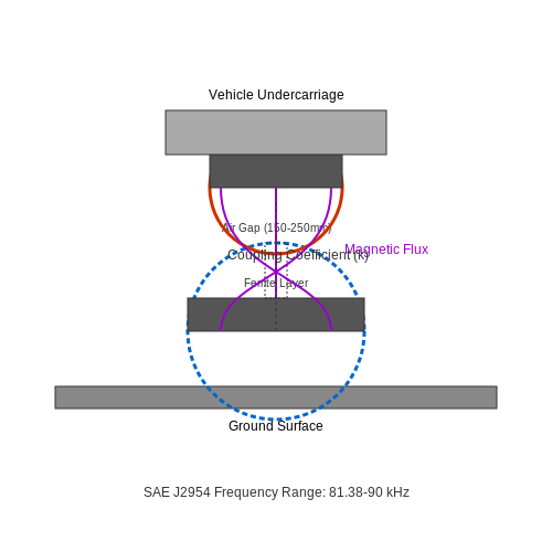
Wireless power transfer (WPT) for electric vehicles (EVs) primarily relies on resonant inductive coupling to achieve efficient energy transmission across an air gap. The system consists of a ground-based transmitting coil and an onboard receiving coil, tuned to the same resonant frequency to maximize power transfer efficiency.
Resonant Inductive Coupling in EV Charging
The power transfer efficiency η between two magnetically coupled coils is governed by:
where k is the coupling coefficient, and Q1, Q2 are the quality factors of the primary and secondary coils, respectively. For EV applications, typical operating frequencies range from 85 kHz (SAE J2954 standard) to 150 kHz, with coupling coefficients between 0.1 and 0.3 depending on coil alignment.
Coil Design Considerations
Circular and DD (double-D) coil topologies dominate EV wireless charging due to their superior misalignment tolerance. The mutual inductance M between coils is calculated as:
where μ0 is the permeability of free space, N represents turn counts, r denotes coil radii, and d is the inter-coil distance. Ferrite shielding is essential for directing magnetic flux and reducing eddy current losses in nearby conductive materials.
Power Electronics Architecture
Modern EV wireless chargers employ a dual-active bridge (DAB) converter topology for bidirectional power flow capability. The system typically includes:
- High-frequency inverter (usually GaN-based for >95% efficiency)
- Series-series or LCL resonant network
- Active rectification with synchronous MOSFETs
- Dynamic impedance matching circuits
The power transfer capability P scales with frequency f and coil current I as:
Alignment and Positioning Systems
Automated alignment using magnetic field sensing and machine vision achieves ±75 mm positional tolerance for 11 kW systems. The SAE J2954 standard specifies three power classes:
| Power Class | Nominal Power | Frequency Range |
|---|---|---|
| WPT1 | 3.7 kW | 81.38-90.00 kHz |
| WPT2 | 7.7 kW | 81.38-90.00 kHz |
| WPT3 | 11 kW | 81.38-90.00 kHz |
Efficiency Optimization Techniques
Modern systems implement adaptive frequency tuning to maintain resonance under varying load conditions. The optimal operating point occurs when:
Practical implementations achieve 92-94% DC-to-DC efficiency at 7.7 kW power levels, with total system efficiency (grid-to-battery) reaching 88-90% in commercial systems like WiTricity's Halo and Qualcomm Halo.
EMI and Safety Considerations
International standards IEC 61980 and SAE J2954 limit magnetic field exposure to 27 μT at 85 kHz. Shielding techniques reduce stray fields to below 6.25 μT at 300 mm from the coil center. Foreign object detection (FOD) systems using temperature sensors and metal detection ensure safe operation.
3.3 Medical Implants and Devices
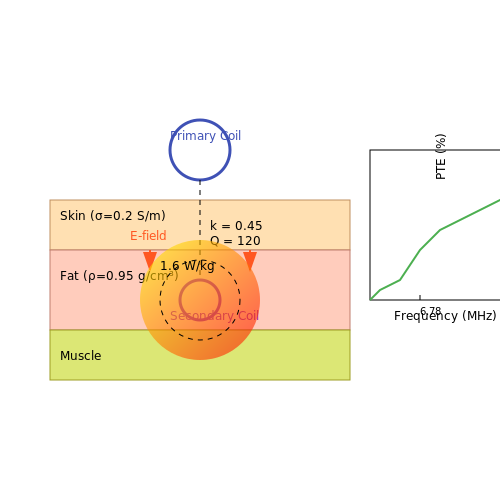
Wireless power transfer (WPT) has revolutionized medical implants by eliminating the need for transcutaneous wires or frequent battery replacements. Inductive coupling and resonant inductive coupling dominate this space due to their efficiency at short ranges (< 5 cm) and biocompatibility. The key challenge lies in optimizing power transfer efficiency (PTE) while ensuring patient safety and minimizing tissue heating.
Inductive Coupling in Implantable Devices
Most implantable medical devices, such as pacemakers, neurostimulators, and cochlear implants, operate at frequencies between 100 kHz and 10 MHz. The power transfer efficiency is governed by the coupling coefficient k and quality factor Q of the coils:
where M is mutual inductance, L1 and L2 are primary and secondary coil inductances, R is parasitic resistance, and ω is angular frequency. For implants, k typically ranges from 0.01 to 0.3 due to coil misalignment and tissue attenuation.
Specific Absorption Rate (SAR) Constraints
Regulatory limits on SAR (e.g., 1.6 W/kg averaged over 1g of tissue in the US) constrain the allowable transmit power. The SAR for a time-harmonic field in tissue is calculated as:
where σ is tissue conductivity (~0.1–2 S/m), E is electric field strength, and ρ is mass density (~1000 kg/m³). This necessitates careful coil design to minimize eddy currents in conductive tissues.
Advanced Techniques
Recent developments include:
- Mid-field WPT: Operates at 1–50 MHz using dipole antennas for deeper penetration (>5 cm) in applications like gastric stimulators.
- Ultrasound-based WPT: Uses piezoelectric transducers at 1–10 MHz, achieving PTE up to 40% through layered tissues.
- Adaptive impedance matching: Dynamically tunes resonance to compensate for coil displacement or tissue property changes.
Case Study: Closed-Loop Spinal Cord Stimulator
The Medtronic Intellis platform employs 32-channel resonant coupling at 6.78 MHz (ISM band) with adaptive power control. The system delivers 2–8 mW continuously while maintaining SAR below 0.5 W/kg, verified through finite-element simulations of EM and thermal distributions in heterogeneous tissue models.
3.4 Industrial and IoT Applications
High-Power Industrial Systems
Wireless power transfer (WPT) in industrial settings eliminates the need for physical connectors in harsh environments, reducing wear and failure risks. Resonant inductive coupling dominates here, with power levels exceeding 10 kW for automated guided vehicles (AGVs) and robotic arms. The efficiency η of such systems is derived from the coupling coefficient k and quality factor Q:
where Q1 and Q2 are the quality factors of the transmitter and receiver coils. For industrial-grade WPT, k typically ranges from 0.2 to 0.6, with Q factors exceeding 1000 in Litz-wire coils.
IoT and Sensor Networks
Far-field RF energy harvesting powers distributed IoT nodes, enabling maintenance-free operation. Rectenna systems convert ambient RF (e.g., Wi-Fi at 2.4 GHz) to DC with efficiencies up to 40% using Schottky diodes. The received power Pr follows Friis’ transmission equation:
where Pt is transmit power, Gt/Gr are antenna gains, and d is distance. Practical deployments use beamforming phased arrays to dynamically power moving sensors.
Case Study: Smart Factory Implementation
A German automotive plant deployed 150 resonant WPT pads (6.78 MHz) for tool-free charging of inspection drones. The system achieves 85% efficiency at 30 cm misalignment tolerance, with Q = 1200 coils and GaN-based inverters.
Energy-Autonomous Industrial IoT
Backscatter communication couples with WPT to create battery-less sensors. Load modulation techniques enable data transmission while harvesting energy, with power budgets as low as 10 µW. The modulation depth m optimizes the trade-off between data rate and harvested energy:
Recent advances include multi-hop RF power routing, where intermediate nodes relay both energy and data.

4. Efficiency and Energy Loss
4.1 Efficiency and Energy Loss
Efficiency in wireless power transfer (WPT) systems is fundamentally governed by the ratio of delivered power to the load versus the input power supplied by the source. The primary sources of energy loss include resistive dissipation in coils, radiative losses, and coupling inefficiencies between transmitter and receiver. The efficiency η is expressed as:
where Pout is the power delivered to the load and Pin is the input power. In resonant inductive coupling, the efficiency is highly dependent on the coupling coefficient k and the quality factors Q1 and Q2 of the transmitter and receiver coils, respectively.
Coupling and Quality Factor
The coupling coefficient k is defined as:
where M is the mutual inductance and L1, L2 are the inductances of the transmitter and receiver coils. The quality factor Q of a coil is given by:
where ω is the angular frequency and R is the series resistance. Higher Q values reduce resistive losses but require precise tuning to maintain resonance.
Loss Mechanisms
Major sources of energy loss in WPT include:
- Ohmic Losses: Resistive heating in coil windings and conductive traces, especially at high frequencies due to skin effect.
- Eddy Currents: Induced currents in nearby conductive materials, leading to parasitic heating.
- Radiation Losses: Energy dissipation as electromagnetic waves, particularly in loosely coupled or misaligned systems.
- Dielectric Losses: Absorption of energy in insulating materials due to molecular polarization effects.
Maximizing Efficiency
To optimize efficiency, the following strategies are employed:
- Impedance Matching: Ensuring the load impedance matches the source impedance to minimize reflections.
- Frequency Tuning: Operating at the resonant frequency to maximize energy transfer.
- High-Q Materials: Using low-loss dielectric substrates and Litz wire to reduce resistive losses.
- Active Compensation: Employing adaptive tuning circuits to counteract detuning caused by environmental changes.
For example, in high-power inductive charging systems, efficiency exceeding 90% can be achieved at close range (< 10 cm) with precise alignment and optimized coil geometries. However, efficiency drops sharply with increasing distance or misalignment due to reduced coupling.
Mathematical Derivation of Optimal Efficiency
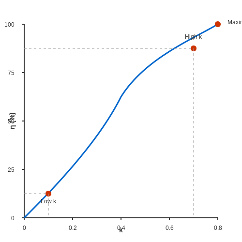
The maximum achievable efficiency ηmax for a resonant inductive link is derived from the general two-port network theory:
This equation highlights the importance of both coupling and quality factors. For weak coupling (k << 1), efficiency scales approximately as k2Q1Q2, emphasizing the need for high-Q coils in loosely coupled systems.
4.2 Safety and Health Concerns
Electromagnetic Field Exposure
Wireless power transfer (WPT) systems generate time-varying electromagnetic fields (EMFs), raising concerns about human exposure. The two primary mechanisms of interaction are:
- Induced currents in tissues: Time-varying magnetic fields (kHz–MHz range) can induce eddy currents in conductive biological tissues, governed by Faraday's law:
where E is the induced electric field and B is the magnetic flux density. For a homogeneous medium, the current density J is:
where σ is tissue conductivity (0.1–1 S/m for most tissues).
Specific Absorption Rate (SAR)
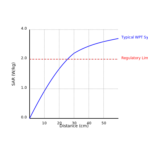
SAR quantifies power absorption per unit mass (W/kg) and is calculated as:
where ρ is tissue density (≈1000 kg/m³). Regulatory limits (e.g., IEEE C95.1-2019) specify:
- 1.6 W/kg averaged over 1g of tissue (FCC limit)
- 2.0 W/kg averaged over 10g (ICNIRP guideline)
Thermal Effects vs. Non-Thermal Effects
At WPT frequencies (typically 20–150 kHz), thermal effects dominate risk assessments. The Pennes bioheat equation models temperature rise:
where k is thermal conductivity, c is specific heat, and q terms represent metabolic heat and blood perfusion.
Mitigation Strategies
Modern WPT systems implement:
- Frequency optimization: Operating below 100 kHz reduces SAR while maintaining efficiency
- Field cancellation: Opposing coil currents minimize stray fields
- Foreign object detection: Real-time impedance monitoring detects living tissue intrusion
Regulatory Compliance
Key standards include:
- IEEE Std C95.1-2019: EMF exposure limits
- IEC 62233: Measurement methods for human exposure
- Qi v1.3 specification: Mandates <15 W/kg peak SAR for inductive charging
Long-Term Biological Effects
While acute thermal effects are well-characterized, research continues on:
- Chronic low-level exposure implications
- Potential non-thermal mechanisms (e.g., radical pair effects)
- Cumulative exposure in multi-device environments
4.3 Distance and Alignment Constraints
Fundamental Limits of Power Transfer Distance
The efficiency of wireless power transfer (WPT) systems degrades rapidly with increasing distance between the transmitter and receiver. This is governed by the inverse-square law for radiative far-field methods and exponential decay for near-field inductive coupling. For inductive systems, the coupling coefficient k between coils is a critical parameter:
where M is mutual inductance, and L1, L2 are the inductances of the transmitter and receiver coils. The power transfer efficiency η can be expressed as:
where Q1 and Q2 are the quality factors of the coils. At distances beyond one coil diameter, k typically falls below 0.1, causing efficiency to drop below 50% even with high-Q resonators.
Alignment Sensitivity in Near-Field Systems
Misalignment between transmitter and receiver coils introduces additional losses through:
- Lateral displacement: Reduces effective coupling area
- Angular misalignment: Creates flux leakage
- Axial separation: Increases reluctance in the magnetic path
The lateral displacement tolerance is approximately D/4 for circular coils of diameter D before efficiency drops by 50%. For example, a 10 cm diameter coil pair maintains >80% efficiency only within ±2.5 cm of perfect alignment.
Far-Field Beamforming Challenges
Directional RF power transfer (e.g., microwave or laser) requires precise alignment between transmitter and receiver. The beam divergence angle θ determines the spot size S at distance d:
For a 5.8 GHz system with 30 cm transmitter aperture, the diffraction-limited beam divergence is approximately 3.5°, resulting in a 1.2 m diameter spot at 10 m distance. This necessitates active tracking systems for mobile receivers.
Practical Compensation Techniques
Modern WPT systems employ several methods to mitigate distance and alignment constraints:
- Adaptive impedance matching: Dynamically tunes resonant frequency to compensate for coupling variations
- Multi-coil arrays: Provides spatial freedom through overlapping magnetic fields
- Beam steering: Phased arrays for RF systems adjust phase to focus energy
- Ferrite shielding: Reduces flux leakage in inductive systems
For electric vehicle charging applications, the SAE J2954 standard specifies ±75 mm lateral tolerance and 100-200 mm air gaps while maintaining 85-90% efficiency at 7.7 kW power levels.
4.4 Regulatory and Standardization Issues
Electromagnetic Interference and Safety Standards
Wireless power transfer (WPT) systems operate at high frequencies, often in the kHz to MHz range, generating electromagnetic fields that must comply with international safety standards. The International Commission on Non-Ionizing Radiation Protection (ICNIRP) and the Institute of Electrical and Electronics Engineers (IEEE) define exposure limits for electric and magnetic fields to prevent biological harm. For example, the ICNIRP 2020 guidelines specify:
where f is the frequency in Hz. Compliance with these limits requires careful coil design, shielding, and power control mechanisms.
Frequency Allocation and Regulatory Bodies
WPT systems must adhere to frequency band allocations set by regulatory agencies such as the Federal Communications Commission (FCC) in the U.S. and the International Telecommunication Union (ITU) globally. Key allocated bands include:
- 6.78 MHz (ISM Band): Widely used for resonant inductive coupling.
- 13.56 MHz (HF RFID Band): Common for mid-range WPT applications.
- 100–205 kHz: Permitted for inductive charging under Qi and SAE J2954 standards.
Operating outside these bands may require licensing or risk interference with communication systems.
Standardization Efforts
Several organizations drive WPT standardization:
- Qi (Wireless Power Consortium): Dominates inductive charging for consumer electronics, ensuring interoperability.
- SAE J2954: Standardizes wireless charging for electric vehicles (EVs), specifying alignment tolerances and efficiency thresholds.
- AirFuel Alliance: Promotes resonant and RF-based WPT, focusing on loose-coupling scenarios.
These standards address power levels (3.7 kW for Qi, up to 22 kW for SAE J2954), frequency tolerance (±1 kHz for Qi), and communication protocols (e.g., backscatter modulation for load detection).
Efficiency and Environmental Regulations
Regulations such as the European Union’s Ecodesign Directive mandate minimum efficiency requirements for WPT systems to reduce energy waste. For instance, Qi-certified chargers must maintain >70% efficiency at 5W output. Dynamic charging systems for EVs face additional scrutiny under ISO 19363:2020, which evaluates electromagnetic emissions and grid compatibility.
Case Study: EV Wireless Charging Compliance
The SAE J2954 standard illustrates the interplay of safety and performance metrics. A compliant 11 kW system must:
- Limit stray magnetic fields to <0.27 µT at 1 m distance.
- Achieve >85% efficiency from grid to battery.
- Support alignment offsets up to ±75 mm laterally.
Field trials under the FCC Part 18 rules further validate compliance with conducted and radiated emissions limits.
5. Advances in Material Science
5.1 Advances in Material Science
The efficiency and scalability of wireless power transfer (WPT) systems are heavily influenced by the materials used in their construction. Recent breakthroughs in material science have enabled significant improvements in coupling efficiency, thermal management, and miniaturization of WPT components. Key advancements include the development of high-permeability ferrites, metamaterials, and high-temperature superconductors.
High-Permeability Ferrites
Ferrite materials, particularly manganese-zinc (MnZn) and nickel-zinc (NiZn) ferrites, have become indispensable in inductive WPT systems due to their high magnetic permeability and low eddy current losses. The relative permeability (μr) of modern ferrites can exceed 10,000, significantly enhancing magnetic flux confinement. The quality factor (Q) of a resonant coil is given by:
where ω is the angular frequency, L is the inductance, and R is the equivalent series resistance. Ferrites reduce R by minimizing hysteresis losses, thereby increasing Q and overall efficiency.
Metamaterials for Near-Field Enhancement
Metamaterials engineered with negative permeability (μ < 0) or permittivity (ε < 0) enable subwavelength focusing of electromagnetic fields. These materials are particularly useful in mid-range inductive and capacitive WPT systems. The effective permeability of a metamaterial can be derived from its unit cell structure:
where F is the filling factor, ω0 is the resonant frequency, and Γ is the damping coefficient. Such materials have demonstrated a 300% improvement in power transfer efficiency at 6.78 MHz in recent experiments.
High-Temperature Superconductors (HTS)
HTS materials like yttrium barium copper oxide (YBCO) exhibit near-zero resistance below critical temperatures (Tc), enabling ultra-high-Q resonant coils. The London penetration depth (λL) governs the magnetic field exclusion in superconductors:
where m is the electron mass, ns is the superfluid density, and e is the electron charge. HTS-based coils have achieved Q factors exceeding 106 in cryogenic WPT systems.
Practical Applications
- Electric Vehicle Charging: MnZn ferrites are used in 11 kW automotive WPT pads to reduce leakage flux and comply with ICNIRP safety guidelines.
- Medical Implants: Metamaterial-enhanced WPT enables efficient powering of deep-tissue implants at 13.56 MHz with SAR levels below 1.6 W/kg.
- Space-Based Solar Power: HTS coils are being tested for kilometer-scale WPT in orbital energy transmission systems.

5.2 Integration with 5G and IoT
Resonant Coupling in 5G-Enabled WPT Systems
The integration of wireless power transfer (WPT) with 5G networks hinges on high-frequency resonant inductive coupling, where the quality factor (Q) of the system is critical. The resonant frequency (fr) must align with the 5G mmWave bands (24–100 GHz) to minimize interference while maximizing efficiency. The power transfer efficiency (η) is given by:
where k is the coupling coefficient, and Q1, Q2 are the quality factors of the transmitter and receiver coils. For 5G backhaul nodes, k is typically below 0.3 due to larger coil separation, necessitating high-Q metamaterials to boost efficiency.
Energy Harvesting for IoT Devices
IoT sensors operating in 5G environments often rely on far-field WPT techniques like RF energy harvesting. The harvested power (Ph) from ambient 5G signals follows Friis’ transmission equation:
Here, Pt is the transmit power, Gt and Gr are antenna gains, λ is the wavelength, d is the distance, and ζ is the rectifier efficiency. At 28 GHz, path loss exceeds 80 dB/m, demanding ultra-low-power IoT designs (< 100 µW) or beamforming-assisted WPT.
Beamforming and Spatial Power Distribution
5G phased arrays enable dynamic beam steering for WPT, allowing simultaneous energy delivery to multiple IoT devices. The array gain (Garray) for an N-element antenna is:
where ηelement is the per-element efficiency and D is the directivity. Real-world implementations, such as Samsung’s 2022 prototype, achieved 5 W power transfer at 10 meters using 1024-element arrays at 28 GHz.
Coexistence Challenges and Solutions
- Spectrum Allocation: WPT at 5G frequencies requires guard bands to avoid interference with communication channels. The 3GPP Release 17 specifies −36 dBm/MHz as the maximum permissible WPT leakage.
- Thermal Management: High-Q resonators in 5G base stations require superconducting materials (e.g., YBCO thin films) to reduce ohmic losses at mmWave frequencies.
- Regulatory Compliance: FCC Part 15.247 limits effective isotropic radiated power (EIRP) to 4 W for intentional radiators in the 5.8 GHz ISM band.
Case Study: Smart City Deployment
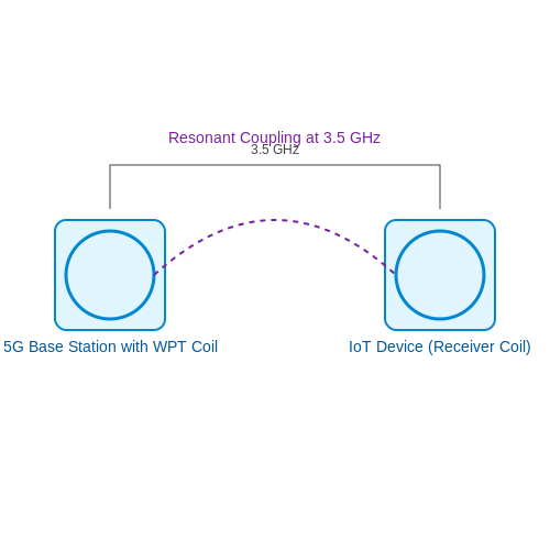
Tokyo’s 2023 pilot project embedded WPT coils in 5G small cells, powering streetlight-mounted IoT air quality sensors. The system achieved 68% efficiency at 3.5 GHz with 15 cm coil separation, demonstrating scalability for urban infrastructure.
5.3 Development of Long-Range Wireless Power
Fundamentals of Long-Range Wireless Energy Transfer
Long-range wireless power transfer (WPT) relies on electromagnetic wave propagation, typically in the form of microwaves or lasers, to transmit energy over distances exceeding several meters. Unlike near-field inductive or resonant coupling, far-field methods exploit radiative principles, where efficiency depends on beam collimation, receiver aperture size, and atmospheric absorption. The Friis transmission equation governs the power received at a distance d:
Here, Pt and Pr are transmitted and received power, Gt and Gr are antenna gains, and λ is the wavelength. Atmospheric losses (e.g., rain fade for microwaves or scattering for lasers) introduce an additional attenuation factor Latm.
Microwave-Based Power Beaming
Microwave WPT (2.45 GHz or 5.8 GHz ISM bands) employs phased-array antennas for directional beamforming. The rectenna (rectifying antenna) converts RF to DC, with efficiency ηrect modeled as:
where Voc is the open-circuit voltage and Rant the antenna impedance. Practical systems, like Japan’s MILAX experiment, achieved 30% end-to-end efficiency at 50 meters using 2.45 GHz.
Laser Power Transmission
Laser WPT uses high-power diodes or fiber lasers (e.g., 808 nm or 1064 nm) with photovoltaic receivers optimized for monochromatic light. The power transfer efficiency is limited by the beam divergence angle θ and PV cell quantum efficiency ηPV:
NASA’s Power Beaming Demonstration (2021) showcased 1.2 kW over 1 km using a 940 nm laser with 40% optical-to-electrical conversion.
Challenges and Mitigations
- Beam Alignment: Adaptive optics (for lasers) and retro-directive arrays (microwaves) compensate for misalignment.
- Safety: Microwave systems must comply with IEEE C95.1-2019 exposure limits; lasers require IEC 60825-1 Class IV controls.
- Efficiency: Multi-junction PV cells and superconducting antennas improve ηsys beyond 60% in lab settings.
Case Study: CASSIOPeiA Satellite
The UK’s Space Solar initiative aims for geostationary satellites beaming 2.45 GHz microwaves to Earth. Theoretical models predict 1 GW transmission at 35% efficiency using 1.5 km diameter phased arrays and 10 km rectenna farms.

6. Key Research Papers and Journals
6.1 Key Research Papers and Journals
- Wireless Power Transfer: Principles and Applications — Wireless Power Transfer Presents a detailed overview of multiple-objective wireless power transfer (WPT) technologies, including the latest research developments and emerging applications Wireless Power Transfer: Principles and Applications offers comprehensive coverage of all key aspects of wireless power transfer (WPT) technologies, including fundamental theory, intelligent control ...
- Bidirectional wireless power transfer: Bridging electric vehicles and ... — Wireless Power Commission standards wireless power transfer. 5W: 120W: Nil: Electromagnetic Inductive Coupling Technique: SAE [144] SAE International has developed a wireless charging standard. 3.7kW: 7.7 kW: 11k W: Magnet Resonance Coupling Technique: A4WP [144] For geographical power, a wireless charging standard: 7.5 kW: 12W: 3.3 kW: Magnet ...
- Advances in EV wireless charging technology - ScienceDirect — Availability and reliability of power supply is a key consideration hence use of existing power network renders, ... 6 (1) (2018), pp. 54-79. View in Scopus Google Scholar [32] ... 2017 IEEE PELS Workshop on Emerging Technologies: Wireless Power Transfer (WoW), IEEE (2017), pp. 295-299. Crossref View in Scopus Google Scholar
- Wireless Power Transfer: Systems, Circuits, Standards, and Use Cases — This paper is organized as follows. In the next section, the most deployed electromagnetic coupled technologies are discussed. In Section 3, electromagnetic uncoupled technologies, including both radio frequency (RF)- and laser-based solutions, are elaborated.We cover acoustic power transfer technologies in Section 4. Section 5 presents technologies that enable improvements in range, power ...
- A comprehensive review of wireless power transfer methods, applications ... — Abstract Wireless power transfer (WPT) is a promising technology that has the potential to revolutionize the present methods of power transmission. ... The remaining 18 pieces are used for introductory descriptions and comprise research articles, review papers, and web portals. ... WPT technology competes with other technologies based on three ...
- Advancements and challenges in wireless power transfer: A comprehensive ... — Wireless power transfer (WPT), inspired by Nikola Tesla's innovative concept in the 1880s, has evolved from conventional wired methods to become a vital, convenient, and safe technology in modern life. 1 Initially, WPT research focused on using microwave technology for long-distance applications like solar space power stations (SSPSs). 2 With the rise of electric devices, the demand for ...
- Wireless power transfer: Applications, challenges, barriers, and the ... — The importance of Wireless Power Transfer (WPT) lies in its potential to make a significant contribution to sustainability. Traditional approaches to the distribution of electricity are associated with substantial inefficiencies, resulting in notable losses during the processes of transmission and storage [1, 2].WPT systems that utilize resonant inductive coupling, radio waves, or other ...
- Wireless power transfer based on novel physical concepts — The first wireless power transfer (WPT) systems date back to the end of the nineteenth century and are rooted in the ideas of Nikola Tesla 1,2,3.In recent years, the rapid expansion of battery ...
- (PDF) A comprehensive review of wireless power transfer methods ... — Wireless power transfer (WPT) is a promising technology that has the potential to revolutionize the present methods of power transmission. This paper aims to provide an overview of WPT, including ...
- Nexus: Nexus - Cell Press — Wireless power transfer (WPT) technology, as a novel power supply method, has brought significant convenience to daily consumption and industrial applications, while providing new means for future energy supply. This paper provides a comprehensive overview of four typical WPT technologies, including physical mechanisms, performance improvement techniques, applications, and discussion. It ...
6.2 Industry Standards and Guidelines
- A comprehensive review of wireless power transfer methods, applications ... — Wireless Power Transfer-Management: PT 63006: Wireless Power Transfer (WPT) Glossary of Terms: PT 63028: Wireless Power Transfer-Magnetic Resonance Interoperability-A4WP Baseline System Specification (BSS) IEC 61980-1 Ed. 1.0: Electric vehicle wireless power transfer (WPT) systems-Part 1: General requirements: IEC 61980-1 Ed. 2.0
- IEC TR 63231:2019 - Consideration of energy efficiency in wireless ... — IEC TR 63231:2019 describes the technical background of current energy efficiency efforts related to wireless power transfer (WPT) technology and commercially available products related to related to audio, video and multimedia systems and equipment. This Technical Report examines use cases, standardization efforts of other standards development organizations (SDOs) and known national regulations.
- Wireless Power Transfer for E-Mobility - 1st Edition - Elsevier Shop — Wireless Power Transfer for e-Mobility: Fundamentals and Design Guidelines for Wireless Charging of Electric Vehicles provides a comprehensive resource for researchers and engineers engaged in the development of automotive WPT systems.. The book opens with an overview of wireless technologies for power transfer and their evolution over time, then focusing on the application of this technology ...
- Wireless Power Transfer: Systems, Circuits, Standards, and Use Cases — This paper is organized as follows. In the next section, the most deployed electromagnetic coupled technologies are discussed. In Section 3, electromagnetic uncoupled technologies, including both radio frequency (RF)- and laser-based solutions, are elaborated.We cover acoustic power transfer technologies in Section 4. Section 5 presents technologies that enable improvements in range, power ...
- Wireless Power Transfer: Systems, Circuits, Standards, and Use Cases - MDPI — Wireless power transfer provides a most convenient solution to charge devices remotely and without contacts. R&D has advanced the capabilities, variety, and maturity of solutions greatly in recent years. This survey provides a comprehensive overview of the state of the art on different technological concepts, including electromagnetic coupled and uncoupled systems and acoustic technologies ...
- PDF Fundamentals of Inductively Coupled Wireless Power Transfer Systems — inductively coupled wireless power transfer (ICWPT) systems. This new technology can be used in various wireless power transfer applications with different specifications, necessities, and restrictions such as in electric vehicles and consumer electronics. A typical ICWPT system involves a loosely coupled magnetic coupling structure and power
- PDF Guide to Industrial Wireless Systems Deployments - NIST — manufacturing systems. This document will only address existing wireless technologies used in industrial environments. Advanced wireless technologies are outside the scope of the document. A revision of the document may be warranted when new and relevant wireless standards and technologies are adopted and used in industry. 1.3 Intended Audience
- Current Research and Future Development on Wireless Power Transfer ... — Dear Colleagues, Wireless power transfer (WPT) is transforming the way power is delivered in our modern world. New advances in WPT promise to extend the range of electric vehicles, improve relability/resilience for electronic devices, reduce surgical frequency for implants, and provide greater utility for the emerging Internet of Things (IoT).
- Wireless power transfer: Applications, challenges, barriers, and the ... — The importance of Wireless Power Transfer (WPT) lies in its potential to make a significant contribution to sustainability. Traditional approaches to the distribution of electricity are associated with substantial inefficiencies, resulting in notable losses during the processes of transmission and storage [1, 2].WPT systems that utilize resonant inductive coupling, radio waves, or other ...
- (PDF) A comprehensive review of wireless power transfer methods ... — Wireless power transfer (WPT) is a promising technology that has the potential to revolutionize the present methods of power transmission. This paper aims to provide an overview of WPT, including ...
6.3 Recommended Books and Online Resources
- Wireless Power Transfer - Wiley-VCH — Chapter 1: The Era of Wireless Power Transfer 1.1 The father of wireless power transfer - Nikola Tesla 1.2 Wireless power Transfer 1.3 About this book Chapter 2: Inductive Power Transfer 2.1 Inductive power transfer 2.2 1-to-1 transmission 2.3 1-to-N transmission 2.4 What are differences between 1-to-1 and 1-to-N transmission Part II: Design
- Wireless Power Transfer: Principles and Applications|Hardcover — Presents a detailed overview of multiple-objective wireless power transfer (WPT) technologies, including the latest research developments and emerging applications ... wireless power transfer and Power-electronic-based impedance matching. Show More. Table of Contents ... 1.3 About this book. Chapter 2: Inductive Power Transfer. 2.1 Inductive ...
- Wireless charging technology and the future of electric transportation ... — Electronic publications. Online. Available online Knovel ... Chapter 1. Introduction. 1.1. Introduction to wireless power transfer technology; 1.2. Wireless power transfer in transportation; 1.3. Micro mobility and wireless power transfer; 1.4. Structure of the book; References; Chapter 2. Green transportation and electric vehicles. 2.1. Future ...
- Wireless Information and Power Transfer: Theory and Practice — Wireless Information and Power Transfer offers an authoritative and comprehensive guide to the theory, models, techniques, implementation and application of wireless information and power transfer (WIPT) in energy-constrained wireless communication networks. With contributions from an international panel of experts, this important resource covers the various aspects of WIPT systems such as ...
- Wireless Power Transfer: Principles and Applications | Wiley — Wireless Power Transfer: Principles and Applications offers comprehensive coverage of all key aspects of wireless power transfer (WPT) technologies, including fundamental theory, intelligent control, configuration analysis, and emerging power electronics techniques. This unique resource is the first book of its kind to provide in-depth ...
- Wireless Power Transfer: Systems, Circuits, Standards, and Use Cases — This paper is organized as follows. In the next section, the most deployed electromagnetic coupled technologies are discussed. In Section 3, electromagnetic uncoupled technologies, including both radio frequency (RF)- and laser-based solutions, are elaborated.We cover acoustic power transfer technologies in Section 4. Section 5 presents technologies that enable improvements in range, power ...
- Wireless Power Transfer for E-Mobility - 1st Edition - Elsevier Shop — Wireless Power Transfer for e-Mobility: Fundamentals and Design Guidelines for Wireless Charging of Electric Vehicles provides a comprehensive resource for researchers and engineers engaged in the development of automotive WPT systems.. The book opens with an overview of wireless technologies for power transfer and their evolution over time, then focusing on the application of this technology ...
- Wireless Information and Power Transfer[Book] - O'Reilly Media — Get full access to Wireless Information and Power Transfer and 60K+ other titles, with a free 10-day trial of O'Reilly. There are also live events, courses curated by job role, and more. Start your free trial
- Wireless power transmission technology and its applications — This book focuses on the basic principles of wireless power transmission technology and the modeling and analysis of related characteristics. The latest research results of the research group on wirel,无线充电 ... Download>Category>Power Management>Others>Wireless power transmission technology and its applications. pdf.
- Wireless power transfer: Applications, challenges, barriers, and the ... — The importance of Wireless Power Transfer (WPT) lies in its potential to make a significant contribution to sustainability. Traditional approaches to the distribution of electricity are associated with substantial inefficiencies, resulting in notable losses during the processes of transmission and storage [1, 2].WPT systems that utilize resonant inductive coupling, radio waves, or other ...