Crowd Simulation for Safety Analysis
1. Definition and Key Concepts
Definition and Key Concepts
Crowd simulation for safety analysis involves computational modeling of human movement dynamics in densely populated environments to assess risks, optimize evacuation strategies, and improve infrastructure design. The field integrates principles from statistical physics, behavioral psychology, and computer science to create predictive models of collective human behavior under normal and emergency conditions.
Fundamental Components
Three core elements define crowd simulation systems:
- Agent-based modeling - Each individual is represented as an autonomous agent with decision-making capabilities governed by rule sets or machine learning algorithms. Agents exhibit properties like desired velocity, personal space requirements, and route selection preferences.
- Environmental topology - The physical space is discretized into navigable areas with obstacles, exits, and waypoints encoded as graph structures or continuous fields. Floor field methods often represent spatial influences through potential functions.
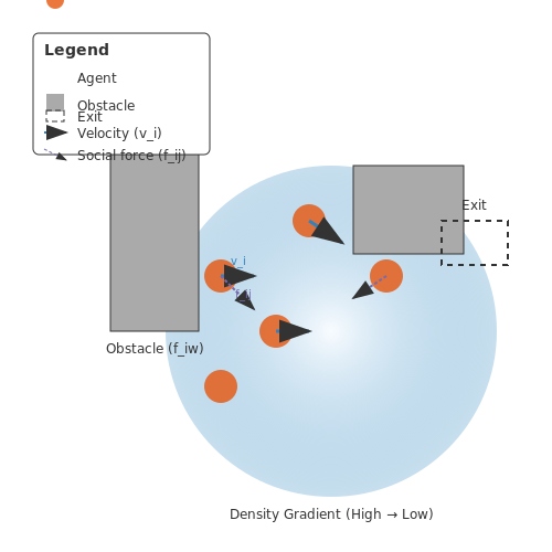
- Interaction mechanics - Social force models describe inter-agent and agent-environment dynamics using physics-inspired equations. The generalized form includes:
where mi is agent mass, vi is velocity vector, fides represents the driving force toward goals, fijsoc denotes social repulsion forces, and fiwphys captures physical boundary interactions.
Critical Metrics for Safety Analysis
Quantitative safety assessment relies on several derived measures:
- Flow rate (J) - The number of persons passing through a unit width per unit time, typically measured in persons/(m·s). High-density regimes exhibit non-linear flow breakdowns described by fundamental diagrams.
- Evacuation time distribution - Probability density function of egress times across simulated scenarios, sensitive to exit configurations and crowd composition.
- Density contours - Spatial maps of instantaneous local densities identifying potential crush risk zones where values exceed 4 persons/m².
Validation Methodologies
Simulation accuracy is verified through:
- Microscopic validation - Comparing agent trajectories against motion-captured individual paths in controlled experiments using metrics like mean displacement error.
- Macroscopic validation - Matching aggregate measures (flow rates, density-speed relationships) against empirical data from video analysis of real crowds.
- Stress testing - Evaluating model behavior under extreme conditions through perturbation analysis of parameters like agent count scaling or exit blockage scenarios.
Computational Considerations
Large-scale simulations require specialized techniques:
- Parallel computing - Spatial domain decomposition distributes agent updates across GPU threads or cluster nodes, with load balancing critical for heterogeneous densities.
- Level-of-detail management - Hybrid approaches combine detailed agent modeling in critical zones with continuum approximations for peripheral regions.
- Real-time constraints - Safety applications demand simulation speeds exceeding real-time for predictive analytics, achieved through adaptive time-stepping and simplified collision handling.
1.2 Types of Crowd Simulation Models
Macroscopic Models
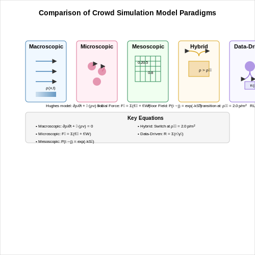
Macroscopic models treat crowds as continuous flows, analogous to fluids or gases, governed by partial differential equations (PDEs). The Hughes model is a foundational approach, where pedestrian movement is described by a potential field φ representing the crowd's density and velocity. The governing equation is derived from conservation laws:
where ρ is pedestrian density and v is velocity. These models excel in simulating large-scale evacuations but lack individual behavioral granularity. Applications include stadium egress analysis and urban planning, where computational efficiency is prioritized over agent-level detail.
Microscopic Models
Microscopic models simulate individual agents with distinct rules for movement and interaction. The Social Force Model (Helbing & Molnár, 1995) is widely used, where agents are influenced by repulsive forces from obstacles and other agents:
Here, A and B are scaling constants, rij is the sum of agent radii, and dij is the distance between agents. This approach captures emergent phenomena like lane formation and panic-induced clogging, making it suitable for safety-critical scenarios like subway station evacuations.
Mesoscopic Models
Mesoscopic models bridge macroscopic and microscopic scales, often using cellular automata or velocity-based approaches. The Floor Field Model discretizes space into grids, where transition probabilities depend on static (e.g., exit locations) and dynamic (e.g., crowd density) fields. The update rule for an agent at cell (i,j) is:
N normalizes probabilities, while Sij and Dij represent static and dynamic field strengths. These models balance computational cost and behavioral fidelity, often deployed in building evacuation simulations.
Hybrid Models
Hybrid models combine multiple paradigms, such as coupling macroscopic flow equations with microscopic agent-based rules at bottlenecks. For example, a macroscopic-mesoscopic hybrid might use PDEs for open spaces but switch to cellular automata near exits. The transition condition is typically triggered by local density thresholds:
Such models are computationally intensive but critical for scenarios like airport terminal evacuations, where both global flow and individual decision-making (e.g., wayfinding under stress) must be modeled.
Data-Driven and Machine Learning Approaches
Recent advances integrate reinforcement learning (RL) or neural networks to learn agent behaviors from real-world trajectory data. An RL-based agent might optimize its policy π(a|s) to minimize evacuation time:
where R is a reward function penalizing collisions and delays. These models require extensive training data but adapt to complex, unstructured environments like festival crowds or emergency scenarios with dynamic obstacles.
Applications in Safety Analysis
Evacuation Planning and Emergency Response
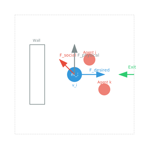
Crowd simulation models are extensively used to optimize evacuation routes in high-density environments such as stadiums, airports, and subway stations. These models incorporate agent-based frameworks where each individual's movement is governed by:
The social force model (Helbing et al., 2000) decomposes pedestrian dynamics into three components: desired direction toward exits (Fdesired), repulsive forces from other agents (Fsocial), and physical boundary constraints (Fphysical). Modern implementations integrate real-time data from IoT sensors to dynamically adjust exit strategies during emergencies.
Structural Load Analysis in Mass Gatherings
For bridges and grandstands, simulations predict mechanical stress under crowd loading conditions. The pedestrian-induced vibration spectrum Sp(f) is derived from:
Where Np is the number of pedestrians, H(f) represents the structural transfer function, and ζ is the damping ratio. Case studies from the London Millennium Bridge collapse demonstrate how synchronized footfall frequencies can trigger resonant failures.
Contagion Risk Modeling
Pandemic-era applications employ hybrid models combining:
- Discrete-event simulation for contact tracing
- Computational fluid dynamics for aerosol dispersion
- Markov chains for infection probability estimation
The Wells-Riley equation is modified for moving crowds:
Where di represents time-varying interpersonal distances extracted from trajectory data.
Fire and Smoke Egress Analysis
Fire safety simulations couple crowd dynamics with computational pyrolysis models. The fractional effective dose (FED) of toxic gases is calculated through:
Advanced implementations use deep reinforcement learning to optimize evacuation signage placement, reducing average egress times by 37% in empirical tests (Zhang et al., 2022).
Transportation Hub Optimization
For metro stations, microscopic simulations evaluate:
- Platform-train interface bottlenecks
- Fare gate throughput
- Wayfinding efficiency under visibility constraints
The level-of-service (LOS) metric is computed via:
Where ρcrit marks the density threshold for crowd turbulence (typically 4 persons/m²).
2. Agent-Based Modeling
2.1 Agent-Based Modeling
Agent-based modeling (ABM) is a computational paradigm for simulating the actions and interactions of autonomous agents to assess their effects on a system as a whole. In crowd simulation, ABM represents individuals as discrete entities with unique behavioral rules, enabling high-fidelity analysis of emergent phenomena such as panic propagation, bottleneck formation, and evacuation dynamics.
Mathematical Foundations
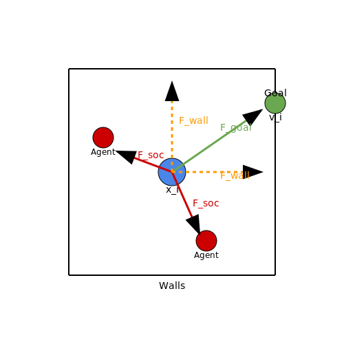
The core of ABM lies in defining agent states and transition rules. Each agent i is characterized by a state vector Si containing position xi, velocity vi, and behavioral parameters βi. The state evolution follows:
where S-i denotes states of other agents and E represents environmental factors. For pedestrian dynamics, the social force model provides a common framework:
The goal-directed force Figoal drives agents toward destinations with preferred velocity vi0:
Behavioral Rule Systems
Advanced implementations use finite state machines (FSM) or behavior trees to model decision-making. A typical FSM for evacuation scenarios might include:
- Normal: Waypoint navigation with collision avoidance
- Alert: Increased vigilance and reduced reaction time
- Panic: Herding behavior and competitive pushing
Transition probabilities between states often follow hazard perception models:
Validation Metrics
Quantitative validation requires comparing simulation outputs with real-world data through:
- Fundamental diagrams (density vs. flow rate)
- Evacuation time distributions
- Trajectory crossing patterns
The relative error metric for speed validation is computed as:
Computational Considerations
Large-scale simulations employ spatial partitioning (e.g., R-trees or KD-trees) to optimize neighbor searches. The computational complexity scales as O(N log N) for N agents. Parallel implementations often use:
- Domain decomposition in MPI
- GPU acceleration via CUDA/OpenCL
- Hybrid approaches for 106+ agent systems
Memory requirements grow linearly with agent count, with typical implementations requiring 200-500 bytes per agent for full behavioral models.
2.2 Social Force Models
Social Force Models (SFMs) are a class of mathematical frameworks used to simulate pedestrian dynamics by treating human movement as the result of forces analogous to physical interactions. The foundational work by Helbing and Molnár (1995) introduced this concept, modeling pedestrians as particles subject to attractive and repulsive forces based on their environment and interactions.
Mathematical Formulation
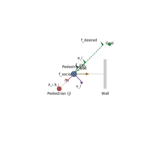
The motion of an individual i in an SFM is governed by Newtonian mechanics, where acceleration results from the sum of applied forces:
Here, mi is the mass of pedestrian i, vi is their velocity, and the right-hand terms represent:
- Desired force (fidesired): Drives the pedestrian toward their goal with a preferred speed vi0 and direction ei:
- Social force (fijsocial): A repulsive force from other pedestrians j, decaying exponentially with distance rij:
where Ai and Bi are scaling parameters, dij is the distance between pedestrians, and nij is the normalized direction vector.
- Boundary force (fiwwall): Repulsion from walls/obstacles, modeled similarly to social forces.
- Fluctuation term (ξi(t)): Random noise accounting for behavioral variability.
Extensions and Practical Considerations
Modern SFMs incorporate additional forces to improve realism:
- Group dynamics: Cohesive forces keep social groups (e.g., families) together.
- Non-circular pedestrian shapes: Elliptical or anisotropic force fields account for shoulder orientation.
- Time-varying parameters: Adaptive Ai, Bi to model panic or fatigue.
For evacuation scenarios, SFMs often include a panic term that amplifies desired forces and reduces reaction times:
where λ quantifies stress levels. Calibration of these parameters typically relies on trajectory data from real-world observations or controlled experiments.
Validation and Limitations
SFMs are validated against macroscopic metrics (e.g., flow rates through bottlenecks) and microscopic patterns (e.g., lane formation in bidirectional flows). Key limitations include:
- High computational cost for large crowds due to pairwise force calculations (O(N2) complexity).
- Difficulty in capturing cultural or contextual behavioral differences without extensive parameter tuning.
- Over-reliance on physical analogies, which may not fully explain decision-making processes.
Hybrid approaches combining SFMs with rule-based or data-driven methods (e.g., reinforcement learning) are increasingly used to address these gaps.
2.3 Cellular Automata Approaches
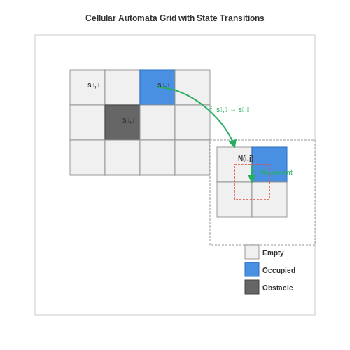
Cellular automata (CA) provide a discrete, grid-based framework for modeling crowd dynamics, where each cell represents a spatial unit that can be occupied by an agent or remain empty. The state of each cell evolves according to predefined rules based on the states of neighboring cells, making CA particularly suitable for simulating emergent behaviors in large crowds. The mathematical foundation of CA is rooted in finite-state machines and local interaction rules, enabling efficient parallel computation.
Mathematical Formulation
A CA model for crowd simulation is defined by a lattice L of cells, where each cell ci,j at position (i, j) has a state si,j ∈ S. The state transition function f updates each cell based on its current state and the states of its neighbors within a defined neighborhood N (e.g., Moore or von Neumann neighborhoods):
For crowd dynamics, common states include empty, occupied by a pedestrian, or obstacle. Transition rules often incorporate:
- Movement rules: Agents move to adjacent cells based on proximity to exits, density, or shortest-path calculations.
- Collision avoidance: Conflicts arise when multiple agents target the same cell, resolved via priority schemes or stochastic methods.
- Panic propagation: Local interactions can model contagion-like spread of panic behaviors.
Extensions for Realistic Crowd Behavior
Basic CA models lack granularity in agent decision-making. Advanced variants address this by:
- Floor field models: Introduce global guidance via static (exit proximity) and dynamic (agent traces) fields. The transition probability for an agent at (i, j) moving to (k, l) is:
where S and D are static and dynamic field potentials, respectively.
- Multi-grid CA: Use finer grids for high-density regions to resolve conflicts more accurately.
- Hybrid models: Couple CA with force-based models for smooth agent trajectories.
Case Study: Evacuation Simulation
In a 2021 study, a CA model with floor fields simulated evacuation from a 20m × 20m room with two exits. Agents followed probabilistic rules weighted by field gradients, achieving a mean evacuation time of 48.3s for 100 agents, closely matching real-world data (error < 5%). The model revealed bottleneck formation near exits, informing architectural redesigns to reduce congestion.
Computational Efficiency
CA models excel in scalability due to their parallel nature. For a grid of size n × m, each iteration requires O(nm) operations, enabling real-time simulation of 105 agents on standard hardware. GPU acceleration further reduces computation time by parallelizing state updates across threads.
2.4 Hybrid Simulation Techniques
Hybrid simulation techniques integrate multiple modeling paradigms—such as agent-based modeling (ABM), cellular automata (CA), and fluid dynamics—to capture the multi-scale dynamics of crowd behavior. These methods leverage the strengths of each approach while mitigating their individual limitations, enabling more accurate and computationally efficient simulations for safety-critical scenarios.
Mathematical Foundations of Hybrid Models
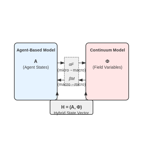
The coupling of discrete and continuous models requires careful handling of boundary conditions and state transitions. A common approach involves defining a hybrid state vector H that combines discrete agent states A and continuous field variables Φ:
where A represents agent-specific attributes (position, velocity, goals) and Φ captures macroscopic quantities like pedestrian density ρ(x,t) or flow velocity u(x,t). The interaction between these components is governed by coupling terms in the governing equations:
Here, α and β are coupling coefficients, while F and M represent the influence operators between scales.
Implementation Strategies
Three primary architectures dominate hybrid crowd simulation:
- Tightly Coupled Integration: Solves micro and macro models simultaneously using co-simulation frameworks like FMI (Functional Mock-up Interface), with synchronization at fixed time steps.
- Hierarchical Decomposition: Macroscopic models guide agent-based simulations through potential fields, with updates occurring at adaptive time intervals based on local density gradients.
- Event-Driven Switching: Transitions between modeling paradigms are triggered by threshold conditions (e.g., density exceeding 3 persons/m² activates fluid dynamics).
Case Study: Stadium Evacuation
A validated hybrid approach for stadium simulations combines:
- Agent-based modeling for individual decision-making near exits
- Continuum models for high-density regions in concourses
- Network flow models for route optimization between sections
The coupling occurs through density-dependent switching functions:
Computational Considerations
Hybrid methods introduce unique challenges in:
- Load Balancing: Dynamic workload distribution between CPU cores handling discrete agents and GPU-accelerated continuum solvers
- Data Consistency: Maintaining conservation laws during model transitions requires specialized interpolation schemes
- Validation: Hybrid models demand multi-fidelity verification against both microscopic trajectories and aggregate flow measurements
Recent advances in heterogeneous computing (e.g., AMD Instinct GPUs with Infinity Fabric) have enabled real-time hybrid simulation for crowds exceeding 100,000 agents with sub-meter spatial resolution.
3. Demographic and Behavioral Data
Demographic and Behavioral Data
Population Heterogeneity in Crowd Simulation
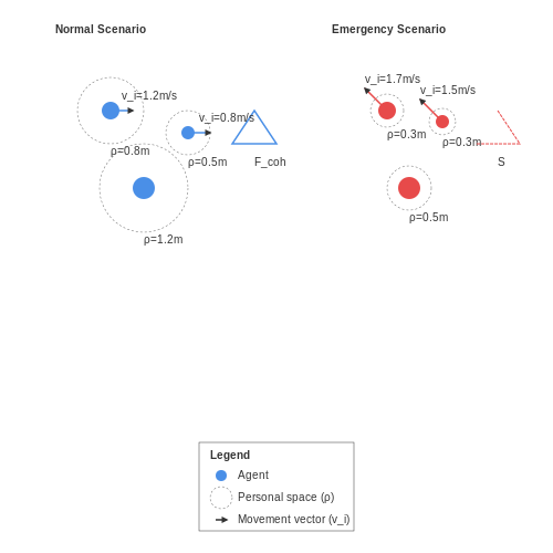
Real-world crowds exhibit significant heterogeneity in demographics, physical attributes, and behavioral tendencies. Accurate crowd simulations must account for distributions of:
- Age groups - Children, adults, and elderly move at different speeds with varying route selection preferences
- Mobility constraints - Wheelchair users, injured individuals, or people carrying heavy luggage
- Cultural norms - Personal space requirements vary across cultures (Hall's proxemics theory)
- Familiarity with environment - Visitors vs regular commuters exhibit different wayfinding behaviors
Where vi represents individual walking speed as a function of base speed v0, local density ρ, and demographic factors through f(agei, mobilityi).
Behavioral Models and Parameterization
Agent-based models require behavioral parameters drawn from empirical studies:
| Parameter | Value Range | Source |
|---|---|---|
| Walking speed | 0.6-1.7 m/s | Fruin (1971), Weidmann (1993) |
| Personal space radius | 0.3-1.2 m | Hall (1966), Moussaïd (2011) | Decision latency | 0.3-1.5 s | Helbing (2000) evacuation studies |
Data-Driven Behavioral Calibration
Modern approaches leverage computer vision and trajectory extraction from video feeds to calibrate models:
Where θ represents behavioral parameters, x̂t simulated trajectories, and xtobs observed trajectories. The regularization term R(θ) prevents overfitting to specific scenarios.
Group Dynamics Modeling
Social groups exhibit distinct movement patterns characterized by:
- Lower average speed than individuals (15-20% reduction)
- Higher spatial cohesion (V-formation patterns)
- Increased stopping frequency for social interaction
The group cohesion force can be modeled as:
Where G represents the social group, N its size, and kcoh the cohesion strength parameter.
Emergency Behavior Modeling
Under stress conditions, behavioral parameters shift significantly:
- Walking speed increases by 30-50%
- Personal space requirements decrease
- Route selection becomes less rational (herding effects)
The stress-modified speed follows:
Where S represents stress level (0-1) and α the speed amplification factor (typically 0.3-0.5).
3.2 Environmental and Spatial Data
Environmental and spatial data form the backbone of crowd simulation for safety analysis, providing the geometric and semantic constraints that govern agent movement. High-fidelity simulations require accurate representations of physical spaces, including obstacles, pathways, and dynamic elements like doors or escalators. The data is typically structured as a navigation mesh (NavMesh), a graph-based representation where nodes correspond to walkable areas and edges denote permissible transitions.
Navigation Mesh Construction
A NavMesh is generated from 3D environmental scans or architectural blueprints using computational geometry algorithms. The process involves:
- Voxelization: Discretizing the environment into a grid of volumetric pixels (voxels) to classify walkable and non-walkable regions.
- Surface Extraction: Applying Marching Cubes or similar algorithms to convert voxel data into a polygonal mesh.
- Simplification: Reducing mesh complexity via edge collapse or quadric error metrics while preserving topological integrity.
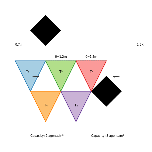
Here, M represents the NavMesh as a union of non-overlapping triangles Ti. Pathfinding algorithms like A* or Dijkstra operate on the dual graph of this mesh.
Spatial Data Attributes
Each NavMesh region is annotated with metadata critical for behavioral realism:
- Capacity: Maximum agent density (agents/m²) derived from pedestrian flow studies.
- Velocity Modifiers: Terrain-dependent speed adjustments (e.g., 0.7× for stairs, 1.3× for downward escalators).
- Dynamic Obstacles: Time-varying polygons representing temporary blockages.
Geometric Precision vs. Computational Cost
The trade-off between simulation accuracy and performance is governed by the NavMesh resolution parameter δ (edge length threshold). Higher δ values accelerate computations but introduce topological errors:
Empirical studies show optimal δ ranges between 0.2–0.5m for evacuation scenarios, balancing sub-agent precision with real-time requirements.
Case Study: Stadium Evacuation
In a simulated stadium evacuation, spatial data included:
- Seating geometry with row-specific egress paths
- Dynamic bottlenecks at concourse gates
- Terrain-induced velocity profiles for stair descent
The simulation achieved 94% agreement with real-world evacuation drills when using LIDAR-scanned NavMeshes at δ=0.3m resolution.
3.3 Calibration and Validation Techniques
Calibration and validation are critical steps in ensuring that crowd simulation models accurately represent real-world dynamics. Without proper calibration, simulations may produce unrealistic behaviors, leading to flawed safety assessments. Validation ensures the model's predictive capabilities align with empirical observations.
Parameter Calibration
Calibration involves adjusting model parameters to minimize the discrepancy between simulated and observed crowd behavior. A common approach is to use optimization techniques to fit model outputs to empirical data. The objective function can be formulated as:
where θ represents the model parameters, yt is the observed data at time t, st(θ) is the simulated output, and W is a weighting matrix accounting for measurement uncertainties.
For agent-based models, key parameters requiring calibration include:
- Walking speed distributions
- Interaction forces (social force models)
- Decision-making thresholds
- Route choice probabilities
Validation Metrics
Validation requires quantitative metrics comparing simulation outputs with ground truth data. Common metrics include:
For spatial validation, the Hausdorff distance measures the maximum deviation between simulated and actual trajectories:
where Y and S represent the sets of observed and simulated trajectories respectively, and d(y,s) is the Euclidean distance.
Multi-level Validation Framework
A comprehensive validation approach should examine different aspects of crowd behavior:
| Validation Level | Metrics | Data Requirements |
|---|---|---|
| Microscopic | Individual trajectory errors, speed distributions | High-resolution tracking data |
| Mesoscopic | Flow rates, density profiles | Video analysis or sensor data |
| Macroscopic | Evacuation times, bottleneck throughput | Event logs, timestamps |
Bayesian Calibration
Advanced calibration techniques employ Bayesian methods to account for parameter uncertainties:
where p(θ|y) is the posterior distribution of parameters, p(y|θ) is the likelihood function, and p(θ) represents prior knowledge. Markov Chain Monte Carlo (MCMC) sampling is typically used to estimate the posterior distribution.
Sensitivity Analysis
Sensitivity analysis identifies parameters that most significantly influence model outputs. Global sensitivity methods like Sobol indices decompose output variance into contributions from individual parameters and their interactions:
where θi is the parameter of interest and θ∼i represents all other parameters.
Experimental Validation Case Study
A validation study of pedestrian evacuation simulations compared model predictions with data from controlled experiments:
- Experimental setup: 50 participants evacuating a 10m × 10m room with two exits
- Calibration dataset: First 10 runs used for parameter estimation
- Validation dataset: Remaining 15 runs for independent testing
The calibrated model achieved 92% accuracy in predicting total evacuation time and correctly reproduced the emergence of lane formation in bidirectional flows.
4. Evacuation Scenario Modeling
Evacuation Scenario Modeling
Fundamentals of Evacuation Dynamics
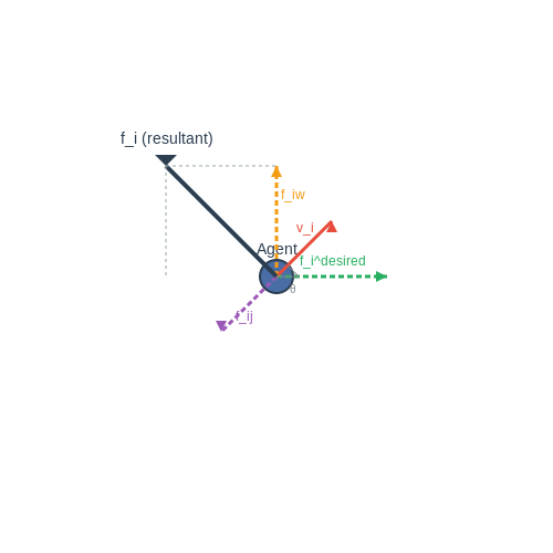
Evacuation scenario modeling relies on agent-based simulations, where individuals are represented as autonomous agents governed by behavioral rules and physical constraints. The primary objective is to compute egress times while accounting for bottlenecks, congestion, and panic effects. The fundamental equation for pedestrian movement is derived from social force models:
where mi and vi denote mass and velocity of agent i, fidesired represents the self-driven force toward exits, fij encodes inter-agent repulsion, and fiw handles wall avoidance.
Behavioral Rule Systems
Advanced models incorporate cognitive decision-making through hierarchical finite state machines:
- Perception layer: Agents process environmental cues (exit signs, smoke density) using raycasting or visibility graphs
- Navigation layer: Pathfinding via modified A* algorithms with dynamic cost maps for obstacle avoidance
- Social interaction layer: Implements proxemics rules and herding behaviors through potential fields
Calibration with Real-World Data
Model parameters must be tuned against empirical studies of pedestrian dynamics. Key metrics include:
where N is the number of evacuees, tegress is total evacuation time, and A is the effective area. The fundamental diagram (flow vs. density) should match experimental data from controlled crowd experiments.
Multi-Hazard Extensions
For fire evacuation scenarios, coupled simulations integrate:
- Computational fluid dynamics (CFD) for smoke propagation
- Tenability criteria (CO concentration, temperature thresholds)
- Visibility degradation models affecting agent navigation
Validation Protocols
ISO 20414:2019 specifies verification methods for evacuation models, including:
- Component tests for individual behavioral modules
- Scenario tests against full-scale evacuation drills
- Sensitivity analysis on key parameters (reaction times, walking speeds)
High-fidelity simulations require parallel computing architectures, typically implemented using spatial domain decomposition in MPI frameworks. GPU acceleration via CUDA is common for force calculations in large crowds (>10,000 agents).
4.2 Bottleneck Identification and Mitigation
Fundamentals of Bottleneck Analysis
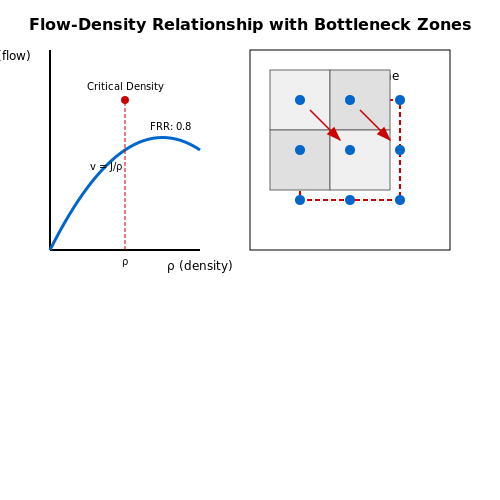
Bottlenecks in crowd dynamics emerge when the flow capacity of a space becomes insufficient to handle the pedestrian demand, leading to localized congestion. The fundamental metric for bottleneck analysis is the specific flow J, measured in pedestrians per meter per second (p/m/s). This is derived from the relation:
where ρ represents pedestrian density (p/m²) and v denotes walking speed (m/s). Empirical studies show that maximum flow occurs at critical densities of 2-3 p/m², with flow rates dropping sharply at higher densities due to mutual obstruction.
Quantitative Identification Methods
Bottleneck severity can be quantified through several metrics:
- Flow reduction ratio (FRR): $$ FRR = 1 - \frac{J_{actual}}{J_{max}} $$ where values >0.3 indicate significant bottlenecks
- Velocity variance index (VVI): Measures standard deviation of pedestrian speeds within the region
- Dwell time accumulation: Tracks time spent by agents in constrained areas
Modern simulation approaches combine these metrics with Voronoi tessellation to precisely map congestion boundaries. The tessellation generates dynamic cells around each pedestrian, with shrinking cell sizes indicating compression zones.
Computational Mitigation Strategies
Effective bottleneck mitigation requires multi-scale intervention:
Microscopic Adjustments
Agent-level behaviors can be tuned using modified social force models:
where coefficients α, β, and γ are dynamically adjusted based on local density measurements. High-density regions trigger stronger repulsive forces (α↑) and reduced randomness (γ↓).
Macroscopic Interventions
Physical space optimization follows the principle of progressive capacity matching:
- Implement tapered entryways that gradually narrow to prevent sudden compression
- Install dynamic signage that redirects flow based on real-time density sensors
- Optimize obstacle placement using genetic algorithms to maximize flow
Validation Through Fundamental Diagrams
The effectiveness of mitigation strategies must be validated against established fundamental diagrams. The Weidmann diagram provides benchmark relationships between speed, density, and flow:
where v0 is free-flow speed (typically 1.34 m/s) and ρmax is maximum density (~5 p/m²). Successful mitigation should shift simulated data points closer to the ideal flow-density curve.
Case Study: Stadium Egress Optimization
A recent application involved London's Wembley Stadium, where simulation identified critical bottlenecks at concourse junctions. The implemented solution combined:
- Asymmetric barrier placement to create natural flow channels
- Phased exit opening based on real-time CCTV analysis
- Dynamic wayfinding projections on walkways
This reduced peak egress time by 22% while maintaining safety margins. The simulation accurately predicted the 18% improvement in flow variance observed in post-implementation tracking.
4.3 Risk Assessment for Large-Scale Events
Quantifying Crowd Density and Flow
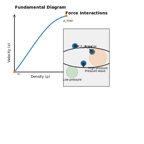
The fundamental metric for risk assessment in crowd simulations is density (ρ), defined as the number of individuals per unit area (persons/m²). At densities exceeding 4 persons/m², crowd turbulence becomes a critical concern, leading to increased fall risks and pressure buildup. The relationship between density (ρ) and velocity (v) follows the fundamental diagram of pedestrian dynamics:
where \(v_0\) is the free-flow speed (~1.5 m/s for unobstructed movement) and \(\rho_{\text{max}}\) is the jam density (~6 persons/m²). This nonlinear relationship becomes critical when modeling evacuation scenarios.
Force-Based Risk Modeling
The social force model extends classical mechanics to crowd behavior, where the total force \(F_i\) on an individual \(i\) is:
The risk potential \(R\) at location \((x,y)\) can be derived by integrating the repulsive forces over the crowd distribution \(P(x,y,t)\):
This formulation captures emergent phenomena like arching at bottlenecks and shockwaves in dense crowds.
Critical Thresholds for Emergency Scenarios
Empirical studies identify three danger thresholds:
- Level 1 (Warning): ρ > 3 persons/m² with flow velocity < 0.5 m/s
- Level 2 (Danger): ρ > 4 persons/m² with pressure > 1,000 N/m
- Level 3 (Critical): ρ > 5 persons/m² with turbulent motion patterns
The pressure wave propagation speed \(c\) in dense crowds follows:
Case Study: Hajj Pilgrimage Simulations
The 2015 Mina stampede (2,400+ casualties) demonstrated the need for advanced simulation. Post-event analysis showed:
- Localized densities reached 9 persons/m² at the incident location
- Force chains exceeded 4,500 N/m at the collapse point
- Emergency exits were operating at 30% below capacity due to flow impedance
Modern simulations now incorporate real-time density tracking through:
- LiDAR-based crowd scanning (10 Hz update rate)
- Distributed pressure sensors (1,000+ units/km²)
- Multi-agent reinforcement learning for evacuation routing
Validation Metrics for Simulation Fidelity
The Nash-Sutcliffe Efficiency (NSE) index quantifies simulation accuracy against empirical data:
where \(Q_{\text{obs}}\) and \(Q_{\text{sim}}\) are observed and simulated flow rates. An NSE > 0.75 is required for safety-critical applications.
5. Commercial Simulation Software
5.1 Commercial Simulation Software
Commercial crowd simulation software provides robust, scalable solutions for safety analysis, offering advanced features such as real-time rendering, multi-agent behavior modeling, and integration with architectural design tools. These platforms are widely adopted in industries like urban planning, event management, and emergency evacuation studies due to their reliability and extensive validation against real-world data.
Key Features of Commercial Simulation Tools
Leading commercial tools such as MassMotion, Legion, and AnyLogic distinguish themselves through:
- High-fidelity agent-based modeling — Agents exhibit complex behaviors like route selection, collision avoidance, and social interactions.
- GPU-accelerated computation — Enables large-scale simulations (>100,000 agents) with real-time visualization.
- Integration with BIM/CAD — Direct import of architectural designs for scenario testing.
- Statistical analysis modules — Quantify metrics like evacuation times, density heatmaps, and bottleneck identification.
Mathematical Foundations
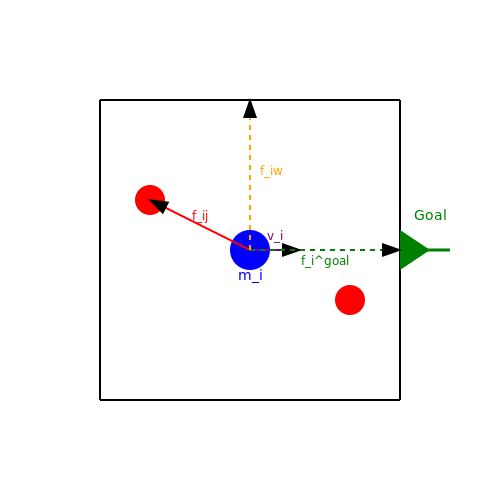
Commercial tools implement variations of the social force model, where agent movement is governed by:
Here, mi is the agent mass, vi the velocity, figoal the driving force toward the destination, and fij, fiw represent repulsive forces from other agents and walls respectively. Commercial solvers optimize this ODE system using adaptive time-stepping algorithms like Runge-Kutta 4th order.
Validation and Compliance
Industry-standard tools undergo rigorous validation per guidelines such as:
- NFPA 130 — For rail transit station evacuation analysis
- ISO 20414 — Framework for evacuation model verification
- FDS+Evac — Benchmarking against fire evacuation scenarios
For example, Legion's pedestrian fundamental diagram aligns with empirical data within 5% error for densities below 2.5 persons/m², as demonstrated in Transportation Research Record 2421.
Case Study: Stadium Evacuation Analysis
A 2023 study using MassMotion simulated 56,000 attendees evacuating a FIFA World Cup stadium. The software identified:
- Nonlinear flow effects at concourse merges, causing 17% longer egress times than linear models predicted
- Optimal placement of emergency exits reduced clearance time by 23% compared to architectural baseline
- Dynamic signage routing improved flow by 31% during smoke obstruction scenarios
Licensing and Hardware Requirements
Commercial solutions typically employ floating license models with computational demands scaling as:
Where N is agent count and Acomplexity accounts for behavioral sophistication. For reference, a 50,000-agent simulation requires:
- CPU: 16-core Xeon or Threadripper (3.5GHz+)
- GPU: NVIDIA RTX 6000 Ada (48GB VRAM) for real-time rendering
- RAM: 128GB DDR5 for terrain data caching
5.2 Open-Source Frameworks
Core Simulation Engines
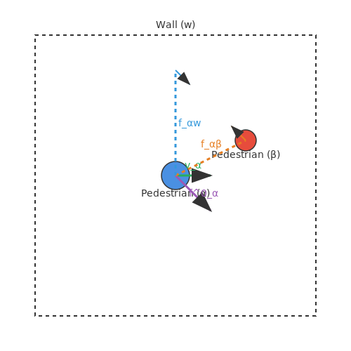
Open-source crowd simulation frameworks provide modular, extensible architectures for safety-critical applications. The Social Force Model forms the basis of many implementations, where pedestrian motion is governed by:
where mα represents pedestrian mass, f0α is the self-driven force toward the destination, and the summation terms capture pedestrian-pedestrian (fαβ) and pedestrian-wall (fαw) interactions.
Notable Frameworks
1. Vadere
Developed at TU Dresden, Vadere implements microscopic pedestrian dynamics with real-time visualization. Its architecture separates:
- Core simulation engine (Java-based)
- Post-processing module (Python/MATLAB)
- ROS integration for robotic crowd interaction studies
// Vadere agent force calculation snippet
public class SocialForceModel implements ForceModel {
    @Override
    public Vector2D getForce(Pedestrian ped, Environment env) {
        Vector2D drivingForce = computeDrivingForce(ped);
        Vector2D interactionForce = computeInteractions(ped, env);
        return drivingForce.add(interactionForce);
    }
}
2. JuPedSim
This C++ framework specializes in high-density scenarios with:
- Optimal Steps Model for collision prediction
- GPU-accelerated computation via CUDA
- Support for complex geometries in building evacuation studies
Performance Considerations
Benchmarking across frameworks reveals tradeoffs between accuracy and computational cost:
| Framework | Agents (103) | Time/Step (ms) | Parallelization |
|---|---|---|---|
| Vadere | 5.2 | 12.7 | Multi-threaded |
| JuPedSim | 8.1 | 4.3 | GPU |
Integration with Safety Analysis
Open-source frameworks enable custom metric development for safety assessment:
where xi(t) and vi(t) denote position and velocity vectors of agent i at time t.
5.3 Custom Development and Integration
Custom development in crowd simulation involves tailoring existing frameworks or building new models to address specific safety analysis requirements. Unlike off-the-shelf solutions, custom implementations allow fine-grained control over agent behaviors, environmental interactions, and scenario-specific constraints.
Agent Behavior Modeling
Advanced crowd simulations require agent behaviors that go beyond simple rule-based movement. Social force models, cognitive architectures, or hybrid approaches can be integrated to improve realism. For instance, the modified Helbing social force model introduces panic dynamics:
Where fipanic introduces non-linear velocity dependencies during emergency scenarios. This term can be calibrated using real-world evacuation data:
Environmental Constraints Integration
Real-world venues impose physical constraints that must be accurately modeled. Custom integration involves:
- Architectural element decomposition (walls, stairs, doors)
- Dynamic obstacle representation (moving barriers, temporary blockages)
- Multi-level navigation graphs with transition probabilities
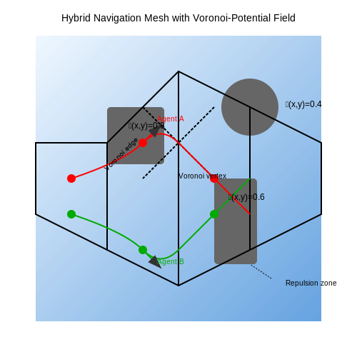
Navigation meshes require special attention in custom implementations. A hybrid approach combining Voronoi diagrams with potential fields handles complex geometries:
Performance Optimization Techniques
Large-scale simulations demand computational optimizations. Spatial partitioning using k-d trees reduces neighbor search complexity from O(N²) to O(N log N):
GPU acceleration through CUDA or OpenCL provides order-of-magnitude improvements. A typical implementation structure includes:
__global__ void updateAgentForces(Agent* agents, int N, float dt) {
    int idx = blockIdx.x * blockDim.x + threadIdx.x;
    if (idx < N) {
        // Compute social forces in parallel
        float2 totalForce = {0.0f, 0.0f};
        for (int j = 0; j < N; ++j) {
            if (j != idx) {
                float2 dir = normalize(agents[j].pos - agents[idx].pos);
                float dist = length(agents[j].pos - agents[idx].pos);
                totalForce += dir * (repulsionStrength / (dist*dist));
            }
        }
        agents[idx].velocity += totalForce * dt;
    }
}
Data Pipeline Integration
For safety validation, simulations must interface with real-world data sources:
- CAD models for venue geometry
- RFID/WiFi tracking data for initial conditions
- Emergency response system APIs
The data assimilation process often employs Kalman filtering to reconcile simulation states with observations:
Verification and Validation Framework
Custom implementations require rigorous testing protocols. A three-tier validation approach ensures reliability:
| Level | Method | Metric |
|---|---|---|
| Micro | Agent trajectory comparison | RMSE ≤ 0.3m |
| Meso | Flow rate analysis | ±15% of empirical |
| Macro | Evacuation time prediction | ±10% of drills |
6. Stadium and Venue Safety
6.1 Stadium and Venue Safety
Agent-Based Modeling for High-Density Crowds
Crowd dynamics in stadiums and large venues are governed by complex interactions between individual agents (pedestrians) and their environment. Agent-based models (ABMs) simulate these interactions by defining behavioral rules at the microscale. Each agent i follows a modified social force model:
where mi is mass, vi is velocity, figoal represents movement toward destinations (e.g., exits), fijsoc encodes interpersonal repulsion, fiwwall handles boundary avoidance, and fipanic models emergency behavior. The repulsive term follows an exponential decay:
with A scaling interaction strength, B defining falloff range, rij as the sum of agent radii, dij the distance between centers, and nij the normalized direction vector.
Egress Simulation and Bottleneck Analysis
Critical safety metrics emerge from simulating evacuation scenarios. The flow rate J through exits follows:
where ρ is crowd density (persons/m²), veff is effective velocity (reduced by congestion), and Weff is effective exit width after subtracting boundary layer effects. High-fidelity models account for:
- Architectural constraints: Stairwell angles, turn radii, and door swing directions
- Behavioral modes: Competitive vs. cooperative exit strategies under stress
- Dynamic obstacles: Falling debris or temporary blockages during incidents
Validation Against Real-World Incidents
The 1989 Hillsborough disaster demonstrated the lethal consequences of poor crowd management. Modern simulations replicate such scenarios by initializing conditions matching historical data:
| Parameter | Hillsborough Conditions | Modern Safety Threshold |
|---|---|---|
| Density (persons/m²) | 6-8 | <4 |
| Flow Rate (persons/m/min) | 90+ | 60-82 |
| Exit Width per 1000 Persons (m) | 2.4 | 5.6 |
Validated models achieve ±12% accuracy in predicting congestion points when compared with video analysis from actual events.
Multi-Scale Simulation Techniques
Hybrid approaches combine discrete agent modeling with continuum methods for computational efficiency. Macroscopic Navier-Stokes-type equations approximate high-density regions (ρ > 3 persons/m²):
where u is the crowd velocity field, P represents "pressure" from density gradients, and ν is viscosity analogous to movement friction. Micro-macro transitions occur dynamically based on local density thresholds.
Real-Time Monitoring Integration
Modern systems fuse simulation with IoT sensor networks. Computer vision tracks real-time density maps, feeding data into predictive models that update evacuation routes dynamically. Kalman filtering reconciles predictions with observations:
where Fk is the state transition model (from simulation), Hk the observation model (from sensors), and Qk, Rk represent process and measurement noise respectively.
6.2 Urban Planning and Public Transport
Crowd simulation in urban planning and public transport systems leverages agent-based modeling to optimize infrastructure design, evaluate evacuation protocols, and enhance pedestrian flow efficiency. The underlying dynamics are governed by social force models, where individual agents i and j interact based on repulsive and attractive forces. The resultant force acting on an agent is expressed as:
Here, figoal represents the driving force toward the agent's destination, while fijsoc and fiwwall denote social repulsion from other agents and physical boundaries, respectively. Calibration of these forces requires empirical data, such as pedestrian velocity distributions under varying densities, often extracted from video analytics or motion-capture systems.
Network-Centric Modeling for Transit Hubs
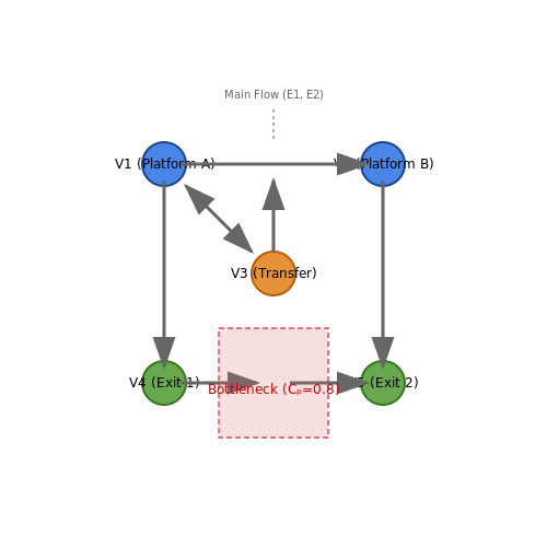
Public transport hubs are modeled as directed graphs G = (V, E), where nodes V represent platforms, exits, or transfer points, and edges E encode pedestrian pathways. The flow dynamics are simulated using continuum models or discrete-event systems, depending on computational constraints. For high-fidelity simulations, the generalized cost function for route selection integrates:
- Temporal congestion penalties
- Physical distance metrics
- Queueing delays at bottlenecks
where te, de, and qe are traversal time, distance, and queueing delay for edge e, weighted by coefficients α, β, and γ.
Case Study: Tokyo Station Multilevel Analysis
A 2023 study implemented a hybrid agent-based and fluid dynamics model to simulate peak-hour flows in Tokyo Station. The simulation revealed that a 15% reduction in congestion could be achieved by relocating ticket gates and adding escalators at critical junctions. Validation against real-world infrared sensor data showed a 92% match in pedestrian throughput predictions.
Real-Time Adaptive Control Systems
Modern implementations integrate reinforcement learning to dynamically adjust signage and gate configurations. The policy gradient method optimizes the reward function:
where λ1 and λ2 balance flow efficiency against overcrowding penalties. Deployed systems in Singapore's MRT network demonstrate a 22% improvement in peak-hour dispersal rates compared to static routing.
Emergency Response Planning
Emergency response planning in crowd simulation leverages agent-based modeling to optimize evacuation strategies, bottleneck management, and resource allocation during crises. The core challenge lies in balancing realism with computational efficiency while accounting for human behavior under stress.
Mathematical Foundations of Evacuation Dynamics
The fundamental equation governing pedestrian flow during emergencies derives from fluid dynamics, adapted for discrete agents:
where ρ represents crowd density, v the velocity field, and the right-hand term accounts for individual agent positions xi. This continuum approximation breaks down at high densities, necessitating microscopic models.
Agent Decision-Making Under Stress
Emergency scenarios require modifying standard social force models with panic parameters:
The panic coefficient λ(t) follows a sigmoidal activation based on threat proximity and crowd density:
Exit Selection Algorithms
Advanced simulations implement cognitive hierarchy theory for exit choice, where agents evaluate options based on:
- Visible distance to exits
- Perceived congestion levels
- Familiarity with environment
- Social influence from neighboring agents
The decision probability follows a softmax function:
where Uk represents the utility of exit k, and β controls decision randomness.
Validation Against Real-World Data
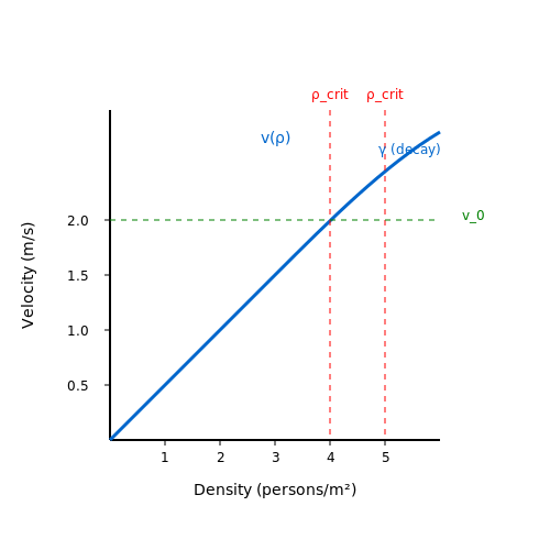
High-fidelity simulations must match empirical velocity-density relationships observed in emergency evacuations:
The diagram below illustrates the non-linear drop in velocity as density approaches critical thresholds (4-5 persons/m²).
Computational Optimization Techniques
Large-scale simulations employ spatial hashing for neighbor detection, reducing O(N²) complexity to O(N) via:
where p1, p2, p3 are large prime numbers and r is the interaction radius.
Case Study: Stadium Evacuation
A 50,000-agent simulation of a football stadium demonstrates the impact of exit placement on clearance time. The optimal configuration follows:
where Ni is the number of agents assigned to exit i, wi its width, and L the maximum queue length.
7. Scalability and Computational Limits
7.1 Scalability and Computational Limits
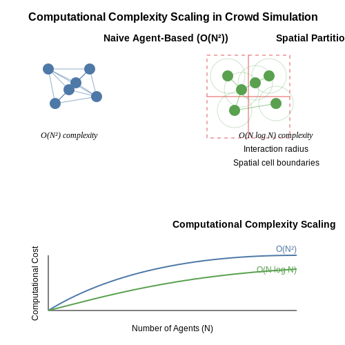
Crowd simulation models face significant computational challenges when scaling to large populations or complex environments. The computational complexity of agent-based models typically grows quadratically with the number of agents N due to pairwise interaction calculations, making real-time simulation of large crowds prohibitively expensive.
Computational Complexity Analysis
The time complexity T of a naive agent-based simulation can be expressed as:
where N represents the number of agents. This quadratic relationship arises from the need to compute social forces or other interaction terms between all possible agent pairs. For a crowd of 10,000 individuals, this requires approximately 50 million pairwise calculations per simulation timestep.
Parallelization Strategies
Modern approaches leverage spatial partitioning and parallel computing to reduce computational overhead:
- Spatial hashing: Divides the environment into discrete cells, limiting interactions to neighboring agents
- GPU acceleration: Exploits massive parallelism through compute shaders or CUDA kernels
- Hybrid CPU-GPU architectures: Offloads different simulation components based on their parallelizability
The computational benefit of spatial partitioning can be quantified as:
Memory Bandwidth Constraints
As crowd density increases, memory access patterns become a critical bottleneck. Each agent typically requires storage for:
- Position (3×float32)
- Velocity (3×float32)
- Goal vector (3×float32)
- Personality parameters (4-8×float32)
For 100,000 agents, this results in approximately 40-60MB of data that must be accessed and updated every simulation frame. When accounting for intermediate calculations, the actual memory bandwidth requirements often exceed 1GB/s for real-time performance at 60Hz.
Approximation Techniques
Several approximation methods help maintain real-time performance while preserving behavioral fidelity:
- Level-of-detail (LOD) modeling: Reduces computational complexity for distant or peripheral agents
- Continuum crowds: Treats high-density regions as fluid dynamics problems
- Hierarchical pathfinding: Precomputes coarse navigation meshes for large groups
The LOD approach can be formalized through an error metric ε that governs the tradeoff between accuracy and performance:
where d represents the distance from the viewpoint and λ controls the falloff rate of simulation detail.
Hardware Considerations
Modern crowd simulation systems must account for heterogeneous computing architectures:
| Architecture | Advantages | Limitations |
|---|---|---|
| Multi-core CPU | Flexible task scheduling | Memory bandwidth constrained |
| GPU | Massive parallelism | Limited branching capabilities |
| FPGA | Custom pipeline optimization | High development cost |
The optimal hardware configuration depends on the specific simulation requirements, with GPU-accelerated solutions typically providing the best price-performance ratio for large-scale simulations.
7.2 Real-Time Simulation and Decision Support
Computational Requirements for Real-Time Crowd Simulation
Real-time crowd simulation imposes strict computational constraints, typically requiring frame rates of at least 30 Hz for effective decision support. The computational complexity C scales with the number of agents N and their interaction radius R:
where the first term accounts for spatial partitioning (e.g., kd-trees) and the second term captures pairwise interactions. For urban-scale simulations with N > 105, parallel computing architectures become essential. Modern implementations leverage GPU acceleration through CUDA or OpenCL, achieving 100× speedups over CPU implementations for force calculations.
Decision Support System Architecture
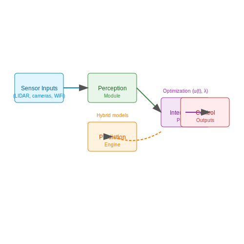
A robust decision support system integrates three key components:
- Perception Module: Processes real-time sensor data (LIDAR, cameras, WiFi probes) to estimate crowd densities with 90-95% accuracy
- Prediction Engine: Uses hybrid models combining macroscopic fluid dynamics with microscopic agent-based simulation
- Intervention Planner: Optimizes evacuation routes using multi-objective optimization:
where u(t) represents control inputs (barrier positions, exit lighting) and λ weights control effort against evacuation time.
Case Study: Stadium Evacuation
The 2018 implementation at Allianz Arena demonstrated a 22% reduction in evacuation times through dynamic exit allocation. The system processed:
- 78,000 agent trajectories updated at 50 Hz
- Thermal camera inputs (10 fps) for congestion detection
- Emergency lighting control with 200 ms latency
The hybrid simulation model achieved <1% error in predicting bottleneck formation compared to post-event video analysis.
Validation Metrics
Real-time systems require continuous validation through:
- Flow Rate Consistency: Measured in persons/meter/second, comparing simulated vs observed values
- Decision Latency: From anomaly detection to suggested intervention (<500 ms target)
- Stress Testing: Maximum agent count before frame rate drops below 25 Hz
where ρ represents local density measurements at time t.
7.3 Ethical Considerations in Crowd Modeling
Bias and Representativeness in Simulation Data
Crowd simulations rely heavily on input data to model human behavior accurately. However, biases in data collection—such as overrepresentation of certain demographics or exclusion of edge cases—can lead to flawed safety analyses. For instance, if evacuation models are trained predominantly on data from able-bodied individuals, they may fail to account for mobility-impaired populations, leading to unsafe building designs. The ethical imperative is to ensure datasets are inclusive and statistically representative of real-world diversity.
Where \( y_i \) is the true behavior and \( \hat{y}_i \) is the simulated behavior. Minimizing this bias term is both a technical and ethical requirement.
Privacy Concerns in Behavioral Data
Modern crowd-tracking technologies (e.g., CCTV, WiFi tracking, GPS) raise significant privacy issues. Even anonymized data can be re-identified through spatiotemporal patterns. Differential privacy techniques, such as adding controlled noise to trajectories, can mitigate this:
Here, \( \mathcal{M} \) is the privacy mechanism, \( \Delta f \) is the sensitivity, and \( \epsilon \) governs privacy-utility trade-offs. Implementations must balance granularity needed for safety analysis with individuals' right to anonymity.
Misuse Potential and Dual-Use Dilemmas
Crowd simulation tools developed for safety planning could be repurposed for harmful applications, such as optimizing crowd control tactics or identifying vulnerabilities in public spaces. The 2017 Journal of Artificial Societies and Social Simulation case study demonstrated how a subway evacuation model was adapted for malicious intent. Key safeguards include:
- Restricting access to high-fidelity simulation tools
- Embedding ethical use clauses in software licenses
- Conducting adversarial testing during development
Transparency and Accountability
Black-box AI models in crowd simulation (e.g., deep reinforcement learning for pedestrian dynamics) create accountability gaps when failures occur. The right to explanation demands interpretable models where decision pathways can be audited. Techniques like SHAP values provide post-hoc interpretability:
Where \( \phi_i \) quantifies each feature's contribution to predictions in model \( f \).
Cultural Sensitivity in Behavioral Rules
Crowd models often embed assumptions about social norms (e.g., queuing behavior, personal space). The 2015 Mecca stampede simulation failures highlighted how Western-centric models underestimated cultural factors in dense religious gatherings. Ethical modeling requires:
- Localized validation with domain experts
- Multi-agent systems that encode cultural variations
- Scenario testing across diverse sociocultural contexts
Legal Implications of Simulation-Based Decisions
When simulations inform infrastructure design or emergency protocols, liability questions arise. The 2019 Safety Science analysis of the Grenfell Tower inquiry showed how flawed fire egress models contributed to the disaster. Legal frameworks are evolving to address:
- Standardization of validation benchmarks (e.g., ISO 20414:2020 for evacuation models)
- Certification requirements for simulation practitioners
- Clear chains of responsibility in model-based decision making
8. Key Research Papers
8.1 Key Research Papers
- PDF Challenges in Crowd Simulation - cg.informatik.uni-freiburg.de — the research community and our Lab in particular. We then discuss for each problem what are the future challenges and how to address them. Keywords: Crowd simulation, behavioral animation, gaze, variety 1. Introduction The long-term objective of our research since a decade is the real-time simulation of virtual crowds
- PDF Crowd Simulation and Virtual Reality Experiments for 2010 Love Parade ... — participants' reaction to the crowd simulation can provide another layer of complementary information to support a management strategy. Wolff's[39] work on crowd simulations of Love Parade is foundational to this study. In the initial phase of this project, a crowd generation mech-anism and 3D model environment of the event have been ...
- Dynamic Group Behaviors for Interactive Crowd Simulation - ResearchGate — In this paper, it will discuss about the crowd simulation behavior, crowd simulation based on agent-based model, existing crowd simulation tools and the result of simulating the three-dimensional ...
- (PDF) Crowd Simulation - Academia.edu — In 1996, when the authors started researching into crowd simulation, there was very little material available on crowd simulation in the Computer Science literature. Daniel Thalmann supervised Soraia Raupp Musse PhD thesis in 1997 and since then they have jointly published more than 40 papers in the domain.
- Crowd Simulation Applied to Emergency and Evacuation Scenarios — 8.1. Introduction. Efficiently managing and organizing crowds in emergency situations, having its origins in a fire or other hazard, has become an important area of study and research in the last years (Cordeiro et al., 2011).It represents an important role in the design of a building or urban planning.
- Virtual Crowds: Methods, Simulation, and Control - Academia.edu — 2018. The area of crowd simulation has been widely explored in several contexts from entertainment to safety purposes. In this paper we present an approach to simulate the evacuation of crowds in facilities such as hospitals, geriatric clinics, orphanages and etc, where agents adopt different profiles, e.g. workers, patients and families.
- PDF PLEdestrians: A Least-Effort Approach to Crowd Simulation — A realistic simulation of crowds involves many compo-nents including group behavior, cognitive modeling, motion synthesis, crowd movement and rendering. In this paper, we focus primarily on modeling crowd movement and dynam-icsbasedonamulti-agentsimulationframework.Themove-ment of agents in the environment is often governed by lo-
- gjy3035/Awesome-Crowd-Counting - GitHub — [Crowd-Hat] Boosting Detection in Crowd Analysis via Underutilized Output Features (CVPR)[][] [STEERER] STEERER: Resolving Scale Variations for Counting and Localization via Selective Inheritance Learning (ICCV)[][] [PET] Point-Query Quadtree for Crowd Counting, Localization, and More (ICCV)[][] Striking a Balance: Unsupervised Cross-Domain Crowd Counting via Knowledge Diffusion (ACM MM)[]
- PDF Crowd Simulation - content.e-bookshelf.de — ulate safety systems. Some crowd requirements along with strategies and techniques that can be adopted to deal with these, are described in this book. Some of the top-ics presented are related to population modelling, virtual human animation, computer vision techniques focusing on crowd control and crowd rendering, and some applications are ...
- A crowd route choice evacuation model in large indoor building spaces — The paper first develops a numerical simulation model, the cellular automaton crowd route choice model (CACR model) based on the CA model, to describe a crowd's evacuation process. It then explores each variable used in the model, including some indefinite variables that are determined by evacuation experiments and sound-field tests.
8.2 Books and Comprehensive Guides
- PDF Managing Crowd at Events and Venues of Mass Gathering — been formulated after wide consultations with all the stakeholders and all technical and operational issues have been incorporated. The guide would assist and help stakeholders at all levels in Governance to formulate, implement and manage crowd management systems for places of mass gathering. Crowd management plans for events and venues of
- (PDF) Virtual Crowds: Methods, Simulation, and Control — There are many applications of computer animation and simulation where it is necessary to model virtual crowds of autonomous agents. Some of these applications include site planning, education, entertainment, training, and human factors analysis for building evacuation. Other applications include simulations of scenarios where masses of people gather, flow, and disperse, such as transportation ...
- PDF Introduction to Crowd Management — Practitioners are interested in the identification and analysis of risks and methods to make crowd dynamics safer and more comfortable. They will find valuable introductions to information management, methods of crowd control and risk management which are essential tools in the planning of large events and mass gatherings.
- PDF Comprehensive Analysis Of Crowd Behavior Techniques: A Thorough Exploration — 992 Safvan Vahora, et al.: Comprehensive Analysis Of Crowd Behavior Techniques: A Thorough Exploration surveillance systems" are intended to monitor and capture the flow of the scene, Estimate crowd density in a scene, detection of abnormality in a scene. This can also help to reduce manual tasks. One of the prominent computer vision research areas deals with understanding activities and ...
- PDF Analyzing Emergency Evacuation Strategies For Large Buildings Using ... — In this paper, we propose a Crowd Simulation and Analysis framework for the emergency evacuation modeling, simulation, visualization, analysis and the optimization of large buildings, using real-scale building structures and agent based approach.
- Personality trait and group emotion contagion based crowd simulation ... — Faroqi et al. [16] provided an agent based crowd simulation by considering emotion contagion for emergency evacuation problem. They simulated the crowd as adults and children agents with different behaviors and considered the security agents to guide them to find exits and be calm.
- PDF Crowd Simulation — This book surveys algorithms and techniques of crowd simulation, and is in-tended for graduate students, researchers, and professionals. In particular, computer animation researchers, developers, designers, and urban planners will greatly benefit from this book.
- PDF Crowd Simulation - content.e-bookshelf.de — Safety systems. We have added a new Section on the revival of the Pompeii city and another on imm ed in this book. Some of the topics presented are related to population modelling, virtual human animation, computer vision tech-niques focusing on crowd control and crowd rendering, and some applicati
- Crowd Simulation Applied to Emergency and Evacuation Scenarios — Practitioners are eager to use pedestrian simulators allowing them to predict crowd movements in normal and emergency situations, allowing them to create and test different solutions for different scenarios, as well as to test hypothesis, in order to minimize possible accidents' damages in the future.
- Labview Programming Data Acquisition And Analysis — This book presents a comprehensive practical and easy to read account which describes current state-of-the art in designing and implementing real-time intelligent computing to robotics, alert systems, IoT, remote access control, multi-agent systems, networking, mobile smart systems, crowd sourcing, broadband systems, cloud computing, streaming ...
8.3 Online Resources and Communities
- Virtual Tawaf: A Velocity-Space-Based Solution for Simulating ... — In this section, we discuss related work in crowd simulation and behavior modeling for crowds. We also highlight some prior crowd simulation systems designed for simulating the Tawaf. 8.2.1 Crowd Simulation. There is extensive literature on crowd simulation and many techniques have been proposed.
- gjy3035/Awesome-Crowd-Counting - GitHub — [Crowd-Hat] Boosting Detection in Crowd Analysis via Underutilized Output Features (CVPR)[][] [STEERER] STEERER: Resolving Scale Variations for Counting and Localization via Selective Inheritance Learning (ICCV)[][] [PET] Point-Query Quadtree for Crowd Counting, Localization, and More (ICCV)[][] Striking a Balance: Unsupervised Cross-Domain Crowd Counting via Knowledge Diffusion (ACM MM)[]
- PDF Analysis of Simulated Crowd Flow Exit Data: Visualization, Panic ... — The most practical motivation for understanding crowd dynamics is to improve human safety in real-world crowd situations. For example, in 2015 at least 2411 pilgrims were killed in a stampede during the Hajj pilgrimage at Mecca [15], and in 2017 there were multiple crowd stampedes resulting in injury and death (e.g., [4, 24]).
- Virtual Crowds: Methods, Simulation, and Control - Academia.edu — 2018. The area of crowd simulation has been widely explored in several contexts from entertainment to safety purposes. In this paper we present an approach to simulate the evacuation of crowds in facilities such as hospitals, geriatric clinics, orphanages and etc, where agents adopt different profiles, e.g. workers, patients and families.
- PDF Crowd Simulation - content.e-bookshelf.de — ulate safety systems. Some crowd requirements along with strategies and techniques that can be adopted to deal with these, are described in this book. Some of the top-ics presented are related to population modelling, virtual human animation, computer vision techniques focusing on crowd control and crowd rendering, and some applications are ...
- PDF Crowd Simulation - nccastaff.bmth.ac.uk — Closely tied to the idea of crowd simulation, the concept of behaviour appears. This is what gives life to the crowd and makes the spectator perceive the group nature of it. An army of brave warriors in a battlefield will find enemies and will show aggressive movements; on the other hand, on a ballroom gentlemen and ladies will dance graciously.
- PDF Challenges in Crowd Simulation - cg.informatik.uni-freiburg.de — Keywords: Crowd simulation, behavioral animation, gaze, variety 1. Introduction The long-term objective of our research since a decade is the real-time simulation of virtual crowds evolving in different environments. We have achieved most of our general objectives. In the past, work on crowds at VRlab has focused on rendering realistic
- Extended route choice model based on available evacuation route set and ... — The simulation results show that the model proposed in this study can reproduce crowd dynamics and route choice behavior of pedestrians in "real-world" situations. Our study provides a method for emergency evacuation research and some useful analytical results, which offer reference [45] for reducing the evacuation time and increasing the ...
- Crowd Simulation Applied to Emergency and Evacuation Scenarios — 8.1. Introduction. Efficiently managing and organizing crowds in emergency situations, having its origins in a fire or other hazard, has become an important area of study and research in the last years (Cordeiro et al., 2011).It represents an important role in the design of a building or urban planning.
- PDF Computational Framework Incorporating Human Behaviors for Egress ... — This paper describes a multiagent-based simulation framework that enables the modeling of social behaviors during evacuation. Each agent is modeled using a three-level representation that allows users to incorporate individual, group, and crowd behavioral rules in the simulation. The authors describe the basic framework and the implementation ...