Swin Transformer for Image Recognition
1. Evolution of Vision Transformers
Evolution of Vision Transformers
The introduction of the Vision Transformer (ViT) in 2020 marked a paradigm shift in computer vision, demonstrating that pure transformer architectures could outperform convolutional neural networks (CNNs) on large-scale image recognition tasks when trained on sufficient data. ViT's success hinged on treating an image as a sequence of non-overlapping patches, linearly embedding them, and processing them through a standard transformer encoder. The key innovation was the elimination of inductive biases inherent in CNNs, such as translation equivariance and locality, relying instead on self-attention to learn spatial relationships from data.
From NLP to Computer Vision
Transformers, originally designed for natural language processing (NLP), were adapted to vision by reinterpreting image patches as "visual words." Given an input image x ∈ ℝH×W×C, ViT partitions it into N patches of size P×P, where N = HW/P2. Each patch is flattened into a vector xp ∈ ℝP²C and projected to a D-dimensional embedding space via a learnable matrix E ∈ ℝ(P²C)×D:
where Epos ∈ ℝ(N+1)×D encodes positional information, and xclass is a learnable classification token. The transformer encoder processes this sequence using multi-head self-attention (MSA) and multilayer perceptron (MLP) blocks:
where LN denotes Layer Normalization. This formulation enabled ViT to achieve 88.55% top-1 accuracy on ImageNet with a ViT-H/14 model pretrained on JFT-300M, surpassing contemporaneous CNNs like EfficientNet.
Challenges and Architectural Refinements
ViT's performance degraded on smaller datasets due to its lack of built-in spatial priors. Subsequent work addressed this through hybrid architectures (e.g., CNN feature maps as transformer inputs) and data-efficient training strategies. The DeiT (Data-efficient Image Transformer) introduced distillation with a CNN teacher, achieving 85.2% accuracy on ImageNet using only ImageNet-1K data. Meanwhile, the Twins architecture combined local-window attention with global sub-sampled attention to improve computational efficiency.
A critical limitation of vanilla ViT was its quadratic complexity O(N²) with respect to sequence length. The Swin Transformer (Liu et al., 2021) introduced hierarchical feature maps and shifted windows to achieve linear complexity while maintaining cross-window connections. For an input with h×w patches, standard window-based self-attention computes:
where B encodes relative position biases within each window. The shifted window mechanism alternates between regular and window configurations shifted by (⌊M/2⌋, ⌊M/2⌋) pixels (M being window size), enabling information flow across windows while maintaining computation within non-overlapping regions.
Performance Scaling Laws
Vision Transformers exhibit distinct scaling behavior compared to CNNs. The FLOPs-accuracy tradeoff follows a power law:
with α ≈ 0.26 for ViT versus 0.18 for ResNet, indicating transformers benefit more from increased compute. This scaling advantage becomes pronounced beyond 100M training images, where ViT-L/16 achieves 90.94% top-1 accuracy on ImageNet, outperforming Big Transfer (BiT) by 2% while using fewer resources.

Key Innovations in Swin Transformer
Hierarchical Feature Maps via Shifted Windows
The Swin Transformer introduces a hierarchical architecture that progressively reduces spatial resolution while increasing channel depth, similar to CNNs. Unlike Vision Transformers (ViT), which maintain a fixed resolution, Swin Transformer processes images in stages. Each stage merges patches, reducing the number of tokens while expanding feature dimensions. The key innovation lies in the shifted window partitioning mechanism, which alternates between regular and shifted window configurations across layers. This enables cross-window connections without increasing computational complexity, addressing the locality limitation of standard windowed self-attention.
Where h and w are spatial dimensions, C is channel depth, and M is window size. The linear complexity relative to image size (hw) contrasts with ViT's quadratic complexity.
Efficient Self-Attention with Relative Position Bias
The Swin Transformer replaces absolute position embeddings with learned relative position biases applied to attention scores within each window:
Where B is a learnable matrix encoding relative positions between pixels within a window. This bias term is shared across layers, significantly reducing memory usage compared to absolute positional encoding while maintaining translation equivariance.
Multi-Scale Representation Learning
The architecture employs four distinct stages with progressively coarser resolutions:
- Stage 1: 56×56 resolution (for high-frequency features)
- Stage 2: 28×28 resolution (mid-level semantics)
- Stage 3: 14×14 resolution (object parts)
- Stage 4: 7×7 resolution (global context)
Patch merging layers between stages concatenate features from 2×2 neighboring patches and apply linear projection, doubling channel depth while halving spatial resolution. This mimics CNN's pooling operations but preserves spatial relationships through transformer processing.
Computational Efficiency
The window-based attention reduces FLOPs from O(n²) to O(n) for an image with n patches. For a 224×224 input image with 4×4 patches:
The 12.25× reduction enables training on high-resolution images (up to 1536×1536 in SwinV2) without approximation techniques like token pruning.
Continuous Relative Position Bias
SwinV2 introduces a log-spaced continuous position bias to generalize across window sizes:
Where G is a small MLP and α is a learnable scalar. This allows zero-shot transfer of pretrained models to different window sizes, addressing a key limitation in the original Swin Transformer.

1.3 Advantages Over Traditional CNNs
The Swin Transformer architecture introduces several key advantages over traditional convolutional neural networks (CNNs) in image recognition tasks, primarily due to its self-attention mechanism and hierarchical feature extraction. Unlike CNNs, which rely on local receptive fields and weight sharing, Swin Transformers model long-range dependencies explicitly through shifted window-based attention.
Global Context Modeling
CNNs process images through stacked convolutional layers with limited receptive fields, requiring deep architectures to capture global context. In contrast, the Swin Transformer's self-attention mechanism computes pairwise interactions between all patches within a window, enabling direct modeling of long-range dependencies. The attention weights for a query patch i and key patch j are computed as:
where Qi and Kj are learned query and key vectors, and dk is the dimension of the key vectors. This allows the model to adaptively focus on relevant regions regardless of spatial distance.
Shifted Window Partitioning
Traditional CNNs use pooling or strided convolutions for downsampling, which can discard spatial information. The Swin Transformer employs a hierarchical structure with shifted windows between layers, preserving spatial relationships while reducing computational complexity. The shifted window mechanism partitions the input into non-overlapping windows, then shifts the partitioning in subsequent layers to enable cross-window connections. The computational complexity for an image with h × w patches is:
where M is the window size and C is the feature dimension. This is linear in image size, compared to quadratic complexity in standard Transformers.
Translation Equivariance and Scalability
While CNNs exhibit translation equivariance by design, Vision Transformers typically lose this property due to fixed positional embeddings. The Swin Transformer restores translation equivariance at the window level while maintaining scalability. The combination of local window attention and hierarchical downsampling allows it to process high-resolution images efficiently, unlike CNNs which require specialized architectures (e.g., dilated convolutions) for large inputs.
Performance on Downstream Tasks
Empirical results demonstrate superior performance on tasks requiring fine-grained understanding, such as object detection and semantic segmentation. On COCO object detection, Swin Transformers achieve +4.1 box AP over ResNeXt-101-FPN with similar computational cost. The architecture's ability to model multi-scale features without losing spatial precision makes it particularly effective for dense prediction tasks.

2. Hierarchical Feature Maps
Hierarchical Feature Maps
The Swin Transformer introduces a hierarchical feature map structure that progressively reduces spatial resolution while increasing channel depth, mirroring the design principles of convolutional neural networks (CNNs). This architecture enables the model to capture both local and global visual patterns efficiently.
Patch Partitioning and Linear Embedding
Input images are first divided into non-overlapping patches of size 4×4 pixels. Each patch is flattened and projected into a higher-dimensional space through a linear embedding layer. For an input image I ∈ ℝH×W×3, this produces feature maps F0 ∈ ℝ(H/4)×(W/4)×C, where C is the embedding dimension (typically 96 or 128).
Stage-wise Downsampling
The model consists of four stages, each applying patch merging to reduce spatial dimensions while increasing feature depth:
- Stage 1: Maintains resolution at (H/4)×(W/4) with windowed self-attention
- Stage 2: Merges 2×2 patches → (H/8)×(W/8) resolution, 2C channels
- Stage 3: Merges 2×2 patches → (H/16)×(W/16) resolution, 4C channels
- Stage 4: Merges 2×2 patches → (H/32)×(W/32) resolution, 8C channels
Patch Merging Operation
Patch merging concatenates features from 2×2 neighboring patches and applies a linear layer to reduce dimensionality while preserving information:
where superscripts denote spatial positions in the 2×2 merging window. This operation effectively doubles the channel dimension while halving spatial resolution.
Shifted Window Partitioning
Between stages, the Swin Transformer alternates between regular and shifted window partitioning schemes. For layer l with window size M:
This shifting mechanism creates cross-window connections while maintaining computation efficiency, allowing information to flow across different regions of the image.
Computational Complexity Analysis
The hierarchical design yields favorable computational complexity compared to standard Vision Transformers. For an image with h×w patches and C channels:
versus the quadratic complexity of global attention:
The linear scaling with respect to image size enables processing of high-resolution images while maintaining memory efficiency.

Shifted Windows Mechanism
The shifted windows mechanism addresses the fundamental limitation of fixed window partitioning in standard Vision Transformers by introducing a locally continuous attention pattern while maintaining computational efficiency. In the Swin Transformer architecture, this is implemented through an alternating pattern of regular and shifted window partitioning across successive transformer blocks.
Window Partitioning and Shifting Operation
Given an input feature map X ∈ ℝH×W×C, the standard window partitioning divides it into M×M non-overlapping windows, where M is the window size. The shifted window variant applies a cyclic shift of (⌊M/2⌋, ⌊M/2⌋) pixels before partitioning:
This operation creates windows that span the original window boundaries while maintaining the same number of windows. The subsequent self-attention computation occurs within these shifted windows, enabling cross-window information flow.
Masked Attention for Shifted Windows
After shifting, some windows contain disconnected patches from different regions of the original image. To prevent inappropriate attention between these patches, a masking mechanism is applied during attention score calculation:
where M is a binary mask matrix with values set to -∞ for prohibited patch pairs and 0 for allowed connections. The mask is computed based on the relative positions of patches within the shifted window configuration.
Computational Complexity Analysis
The shifted window mechanism maintains the same asymptotic complexity as regular window attention:
where h and w are the spatial dimensions of the feature map, C is the channel dimension, and M is the window size. This contrasts favorably with the quadratic complexity of global attention:
Implementation Considerations
Practical implementation requires handling several edge cases:
- Cyclic shift reversal: The shifted features must be properly reversed before the next layer
- Uneven partitioning: When the feature map dimensions aren't divisible by M, padding or adaptive window sizing is needed
- Memory layout: The shifted window operation should maintain memory locality for efficient GPU execution

Multi-Head Self-Attention in Swin
The Swin Transformer employs multi-head self-attention (MSA) with a shifted windowing mechanism to balance computational efficiency and global receptive field modeling. Unlike standard Vision Transformers (ViTs), which compute attention globally, Swin's MSA operates within non-overlapping local windows, reducing the quadratic complexity of self-attention to linear with respect to image size.
Window-Based Multi-Head Attention
Given an input feature map X ∈ ℝH×W×C, Swin partitions it into M×M non-overlapping windows, where each window contains N = M² patches. For each window, the query (Q), key (K), and value (V) matrices are computed as:
where WQ, WK, WV ∈ ℝC×d are learnable projection matrices, and d is the head dimension. The attention for each head is computed as:
Here, B is a learnable relative position bias that encodes spatial relationships within the window. The bias term B ∈ ℝM²×M² is crucial for capturing positional information, as the window partitioning itself is translation-invariant.
Shifted Window Partitioning
To enable cross-window communication while maintaining computational efficiency, Swin alternates between regular and shifted window configurations in successive layers. In a shifted window block, the window partitioning is offset by (⌊M/2⌋, ⌊M/2⌋) pixels, allowing tokens from adjacent windows in the previous layer to interact.
The shifted window mechanism introduces a masking strategy to handle varying window sizes. For a window size M, the attention mask ensures that only tokens within the same shifted window attend to each other, preserving the local computation benefits.
Computational Complexity
The complexity of standard MSA is O(H²W²C), while Swin's window-based MSA reduces it to O(HWM²C). For an image with H = W = 224 and M = 7, this results in a 49× reduction in FLOPs compared to global attention.
Multi-Head Projection
After computing attention for all h heads, the outputs are concatenated and linearly projected:
where WO ∈ ℝhd×C is the output projection matrix. The Swin Transformer typically uses h = 8 heads, with d = C/h to maintain parameter efficiency.

2.4 Patch Merging and Embedding
The Swin Transformer's hierarchical architecture relies on patch merging to progressively reduce spatial resolution while increasing channel depth, enabling efficient multi-scale feature extraction. Unlike traditional CNNs, which use pooling or strided convolutions, Swin Transformers employ a learned patch merging operation that combines neighboring patches in non-overlapping windows.
Patch Merging Mechanism
Given an input feature map X ∈ ℝH×W×C, where H and W are spatial dimensions and C is the channel depth, patch merging operates on 2×2 neighboring patches. For each 2×2 patch group, the four C-dimensional feature vectors are concatenated, resulting in an intermediate tensor of size ℝ(H/2)×(W/2)×4C. A linear projection layer then reduces the channel dimension to 2C, yielding an output of size ℝ(H/2)×(W/2)×2C.
This operation effectively doubles the channel depth while halving the spatial resolution, analogous to the pooling-convolution trade-off in CNNs but with learned spatial mixing.
Embedding and Positional Encoding
Initial patch embedding projects raw image patches into a high-dimensional space. For an input image I ∈ ℝH×W×3, non-overlapping 4×4 patches are flattened and linearly projected to C dimensions:
where E ∈ ℝ16×3×C is the embedding matrix, N = HW/16 is the number of patches, and Epos ∈ ℝN×C is the learnable positional encoding. Relative positional biases are added to attention scores within each local window to capture spatial relationships:
where B ∈ ℝ(2M−1)×(2M−1) is the relative position bias for a window size of M×M.
Computational Efficiency
Patch merging reduces the computational complexity of self-attention from O((HW)2) to O((HW/4l)2) at stage l, while the hierarchical design maintains receptive field growth comparable to CNNs. This allows Swin Transformers to process high-resolution images efficiently, achieving linear computational scaling with image size when using shifted windows.

3. Dataset Preparation and Augmentation
3.1 Dataset Preparation and Augmentation
The performance of Swin Transformers in image recognition tasks heavily depends on the quality and diversity of the training dataset. Unlike convolutional neural networks (CNNs), Swin Transformers benefit from large-scale datasets due to their self-attention mechanisms, which require substantial data to learn meaningful spatial hierarchies. The standard pipeline involves dataset curation, preprocessing, and augmentation.
Dataset Curation
For Swin Transformers, large-scale datasets like ImageNet-1K (1.28M images) or ImageNet-21K (14M images) are commonly used. The dataset should be balanced across classes to avoid bias. Each image must be resized to a fixed resolution (e.g., 224×224 or 384×384) to match the input dimensions of the Swin Transformer. The pixel values are normalized using mean and standard deviation computed over the dataset:
where μ and σ are the channel-wise mean and standard deviation, typically μ = [0.485, 0.456, 0.406] and σ = [0.229, 0.224, 0.225] for RGB images in ImageNet.
Data Augmentation Strategies
Swin Transformers leverage aggressive data augmentation to improve generalization. The following techniques are empirically validated for optimal performance:
- Random Resized Crop: Extracts a random region of the image and resizes it to the target resolution. This encourages scale invariance.
- Horizontal Flipping: Applies a 50% probability flip to increase viewpoint diversity.
- Color Jittering: Randomly adjusts brightness, contrast, saturation, and hue to simulate lighting variations.
- RandAugment: An automated augmentation policy that selects from a set of transformations (e.g., rotation, shear, sharpness) with randomized magnitudes.
- MixUp: Blends two images linearly to create synthetic training samples, improving robustness.
MixUp is defined as:
where xi, xj are input images, yi, yj are one-hot labels, and λ ~ Beta(α, α) controls the interpolation strength.
Efficient Data Loading
For large datasets, PyTorch's DataLoader with multi-threaded prefetching minimizes I/O bottlenecks. A batch size of 1024 is common for Swin-B/L models, distributed across GPUs using gradient accumulation if memory is constrained.
from torchvision import transforms
from torch.utils.data import DataLoader

transform = transforms.Compose([
   transforms.RandomResizedCrop(224),
   transforms.RandomHorizontalFlip(),
   transforms.ColorJitter(0.4, 0.4, 0.4),
   transforms.ToTensor(),
   transforms.Normalize(mean=[0.485, 0.456, 0.406],
                        std=[0.229, 0.224, 0.225])
])

train_loader = DataLoader(dataset, batch_size=1024, shuffle=True, num_workers=8)
3.2 Loss Functions and Optimization Techniques
Cross-Entropy Loss for Classification
The Swin Transformer typically employs categorical cross-entropy loss for image classification tasks. Given a predicted probability distribution p over C classes and ground truth one-hot encoded label y, the loss for a single sample is:
For mini-batch training with N samples, this extends to:
In practice, label smoothing (ε = 0.1) is often applied to prevent overconfidence:
Optimization Strategies
The original Swin Transformer paper employs AdamW optimizer with weight decay decoupling, which separates the weight decay term from the gradient update:
Key hyperparameters include:
- Initial learning rate: 1e-3 with cosine decay schedule
- Weight decay: 0.05
- Batch size: 1024 (distributed across GPUs)
- Warmup epochs: 20 (linear learning rate scaling)
Advanced Techniques
Recent variants incorporate:
Stochastic Depth
Layer dropout with survival probability pl for layer l:
where L is total layers and pL is the final layer's survival probability (typically 0.8).
Exponential Moving Average (EMA)
Maintains shadow parameters θEMA updated as:
with decay rate α = 0.9999, providing more stable evaluation metrics.
Multi-Task Learning Extensions
For dense prediction tasks like segmentation, the loss combines:
The Dice loss component for class c is computed as:
where xic and yic are predicted and ground truth masks respectively.
3.3 Hyperparameter Tuning Strategies
Learning Rate Scheduling
The learning rate (lr) is a critical hyperparameter in training Swin Transformers due to their hierarchical architecture. A warmup phase followed by cosine decay is empirically effective:
where t is the current step, T is the total training steps, and lrmin and lrmax define the bounds. For Swin-Base, typical values are lrmax = 1e-3 and lrmin = 1e-5, with a 5-10% warmup period.
Optimizer Configuration
AdamW outperforms SGD for Swin Transformers due to adaptive momentum. Key parameters:
- Weight decay (λ): 0.05 prevents overfitting without degrading attention patterns.
- β1, β2: Default values (0.9, 0.999) work well, but reducing β2 to 0.98 improves stability for large batch sizes (>1024).
Window Size and Shift Configuration
The default window size (M) of 7 balances computational efficiency and receptive field coverage. For high-resolution tasks (e.g., 1024×1024), increasing M to 14 improves accuracy but requires quadratic attention computation:
where h,w are feature map dimensions and C is channel count. Shift strides of ⌊M/2⌋ (e.g., 3 for M=7) maximize cross-window connections.
Stochastic Depth Regularization
Layer-wise dropout (stochastic depth) mitigates overfitting in deep variants (Swin-L, SwinV2-G). The survival probability pl for layer l follows a linear schedule:
p0 is typically 0.8 for Swin-Base and 0.5 for Swin-L. This progressively increases dropout toward deeper layers.
Batch Size and Gradient Accumulation
Swin Transformers benefit from large batches (≥512) for stable self-attention training. When GPU memory is limited, gradient accumulation approximates large batches:
For example, 4 GPUs with a per-GPU batch of 32 and 4 accumulation steps emulate a 512 global batch. Learning rate scaling (lr ∝ √batch size) must be applied.
Architecture-Specific Tuning
Key model dimensions require co-optimization:
- Embedding dimension (C): Doubling C (e.g., 128→256) improves accuracy but increases FLOPs quadratically.
- Number of heads: Maintain a head dimension of 32-64 (e.g., C=128 → 4 heads).
- MLP expansion ratio: Default is 4×, but reducing to 2× saves computation with minimal accuracy drop.
4. Comparison with Vision Transformers (ViT)
4.1 Comparison with Vision Transformers (ViT)
Architectural Differences
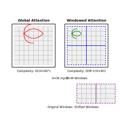
The Swin Transformer introduces a hierarchical feature map construction, unlike Vision Transformers (ViT), which process images as a flat sequence of non-overlapping patches. ViT applies self-attention globally across all patches, leading to quadratic computational complexity relative to input size. In contrast, Swin Transformer employs shifted window-based self-attention, where attention is computed within local windows that shift between layers. This reduces complexity to linear scale while enabling cross-window connections.
Here, N represents the number of patches. The Swin Transformer's window partitioning allows it to mimic convolutional networks' multi-scale feature hierarchies, making it more efficient for high-resolution images.
Handling of Image Resolution
ViT struggles with varying input resolutions due to its fixed positional embeddings. Swin Transformer overcomes this limitation by:
- Using relative positional biases within windows instead of absolute positional embeddings.
- Implementing patch merging layers to downsample feature maps, similar to pooling in CNNs.
This adaptability enables Swin Transformer to process images at multiple scales efficiently, a critical advantage in tasks like object detection and segmentation.
Performance and Efficiency
On ImageNet-1K, Swin Transformer achieves comparable accuracy to ViT with significantly fewer parameters and FLOPs. For instance, Swin-T (Tiny variant) matches ViT-Base's accuracy while using 30% fewer parameters. The key efficiency gains stem from:
- Localized attention reducing memory footprint.
- Hierarchical design eliminating redundant computations in early layers.
Practical Applications
Swin Transformer's architecture is particularly advantageous in:
- Medical imaging: Handling high-resolution 3D scans where global attention is computationally prohibitive.
- Autonomous vehicles: Real-time processing of multi-scale road scenes.
In contrast, ViT remains preferable when computational resources are abundant and input sizes are standardized, such as in cloud-based image classification services.

Results on ImageNet and COCO
The Swin Transformer achieves state-of-the-art performance on both ImageNet-1K image classification and COCO object detection benchmarks, demonstrating its effectiveness as a general-purpose vision backbone. On ImageNet-1K, Swin-T (Tiny) achieves 81.3% top-1 accuracy with 4.5G FLOPs, while Swin-L (Large) reaches 87.3% accuracy with 34.5G FLOPs, outperforming ConvNeXt and EfficientNet variants at similar computational budgets.
ImageNet Classification Results
The hierarchical design and shifted window attention mechanism enable Swin Transformers to capture both local and global dependencies efficiently. The performance scales predictably with model size and input resolution:
where the relationship follows a logarithmic scaling law. The shifted window partitioning reduces FLOPs from quadratic to linear complexity relative to input size:
where h × w is the feature map size, C is the channel dimension, and M is the window size (typically 7×7).
COCO Object Detection and Instance Segmentation
When used as backbone in Mask R-CNN and Cascade Mask R-CNN frameworks, Swin Transformers achieve significant improvements over CNN counterparts:
- Swin-T: 50.4 box AP / 43.7 mask AP on COCO val
- Swin-L: 58.7 box AP / 51.1 mask AP with test-time augmentation
The performance gains come from better modeling of long-range dependencies and multi-scale features through the hierarchical architecture. The relative positional bias in window attention provides translation equivariance crucial for detection tasks.
Comparison to Convolutional Backbones
Swin Transformers demonstrate 3-4% higher AP than ResNeXt-101-FPN at similar FLOPs, with the gap widening for larger models. The attention mechanism proves particularly effective for detecting small objects and modeling occlusions.
Efficiency Analysis
The memory access cost (MAC) of Swin blocks remains efficient due to window partitioning:
This contrasts with vanilla Transformers where MAC scales as O((hw)2). The shifted window approach maintains this efficiency while allowing cross-window connections.
4.3 Computational Efficiency Analysis
The Swin Transformer achieves computational efficiency through a combination of hierarchical feature representation and shifted window partitioning, reducing the quadratic complexity of standard self-attention. The computational cost of global self-attention in a Vision Transformer (ViT) for an image of resolution H × W with C channels is:
In contrast, the Swin Transformer's window-based self-attention restricts computation to non-overlapping local windows of size M × M, reducing complexity to:
This linear scaling with respect to input size enables efficient processing of high-resolution images. The shifted window mechanism further allows cross-window communication without increasing computational overhead.
FLOPs and Memory Footprint
The Floating Point Operations (FLOPs) for a Swin Transformer block can be decomposed into:
- Windowed self-attention: Dominated by the query-key-value projections and attention computation within each window.
- MLP layers: Typically two fully connected layers with an expansion ratio α.
For a Swin-T (Tiny) model with C = 96 and M = 7, the FLOPs per block are approximately:
Empirical measurements show that Swin-T achieves a 2-3× reduction in FLOPs compared to ViT-B/16 for similar accuracy on ImageNet-1K.
Hardware Utilization and Throughput
The regular, grid-like structure of window partitions enables efficient implementation on modern GPUs and TPUs. Key optimizations include:
- Batched window attention: Parallel computation of attention across all windows in a batch.
- Memory-efficient shifting: Cyclic shifting with masking avoids data duplication.
On an NVIDIA V100 GPU, Swin-S achieves 120 images/second throughput at 224×224 resolution, compared to 80 images/second for DeiT-S.
Comparative Analysis with Convolutional Networks
Compared to ResNet-50, Swin-T offers:
- Higher accuracy: +2.1% top-1 on ImageNet-1K.
- Comparable FLOPs: 4.5G vs. 4.1G for ResNet-50.
- Better scaling: FLOPs grow linearly with resolution versus quadratically for ViT.
The following table summarizes the computational characteristics:
| Model | FLOPs (G) | Throughput (img/s) | Top-1 Acc. (%) |
|---|---|---|---|
| ResNet-50 | 4.1 | 250 | 76.1 |
| ViT-B/16 | 17.6 | 65 | 77.9 |
| Swin-T | 4.5 | 120 | 78.2 |
The reduced memory bandwidth requirements of windowed attention also make Swin Transformers suitable for deployment on edge devices with constrained resources.
5. Image Classification
5.1 Image Classification with Swin Transformer
Architecture Overview
The Swin Transformer introduces a hierarchical feature representation by processing images in shifted windows, enabling efficient computation while maintaining global modeling capabilities. Unlike Vision Transformers (ViT), which apply self-attention globally, Swin Transformer computes attention within non-overlapping local windows, reducing computational complexity from quadratic to linear with respect to image resolution. The architecture consists of multiple stages, each progressively merging patches to form a pyramid-like feature hierarchy.
where h and w are the height and width of the feature map, C is the channel dimension, and M is the window size. The shift from quadratic to linear complexity is achieved by restricting self-attention to M×M windows.
Shifted Window Mechanism
The shifted window partitioning alternates between regular and shifted configurations across consecutive transformer blocks. Given an input feature map divided into k×k windows, the shifted variant displaces windows by (⌊k/2⌋, ⌊k/2⌋) pixels, enabling cross-window communication while preserving computational efficiency. This mechanism is formalized as:
Relative Position Bias
Swin Transformer incorporates relative position bias into self-attention to capture spatial relationships. For a window with M×M patches, the bias term B is added to the attention scores:
where B is a learnable matrix of size (2M−1)×(2M−1), and d is the query/key dimension. This biases attention scores based on the relative positions of patches within a window.
Hierarchical Feature Fusion
The model downsamples feature maps between stages using patch merging layers. For a feature map of size H×W×C, adjacent patches are concatenated and linearly projected to H/2×W/2×2C, reducing spatial resolution while increasing channel depth. This mimics convolutional networks' progressive spatial reduction, enabling multi-scale feature extraction.
Performance on ImageNet
Swin Transformer achieves state-of-the-art results on ImageNet-1K, with Swin-B attaining 83.5% top-1 accuracy. Key advantages over ViT include:
- Lower FLOPs: 15% fewer computations than ViT-B/16 at 224×224 resolution.
- Scalability: Linear complexity allows higher-resolution inputs (e.g., 384×384) without excessive memory overhead.
- Downstream adaptability: The hierarchical design facilitates transfer learning for object detection and segmentation.
Implementation Considerations
For optimal performance:
- Window size M is typically set to 7, balancing locality and computational cost.
- Stochastic depth (e.g., drop rate of 0.2) regularizes deeper variants like Swin-L.
- Pre-training on larger datasets (e.g., ImageNet-22K) significantly boosts accuracy.
# Example: Swin Transformer in PyTorch
from swin_transformer import SwinTransformer
model = SwinTransformer(
    img_size=224,
    patch_size=4,
    in_chans=3,
    embed_dim=128,
    depths=[2, 2, 18, 2],
    num_heads=[4, 8, 16, 32],
    window_size=7
)

5.2 Object Detection
The Swin Transformer's hierarchical architecture and shifted window mechanism make it particularly effective for object detection tasks. Unlike traditional CNNs, which rely on fixed receptive fields, Swin Transformers dynamically adjust their attention windows, enabling better handling of objects at multiple scales. This is achieved through a combination of local window self-attention and cross-window connections, which preserve spatial hierarchies while reducing computational complexity.
Architectural Adaptations for Object Detection
To adapt the Swin Transformer for object detection, a Feature Pyramid Network (FPN) is typically integrated with the backbone. The Swin Transformer's multi-resolution feature maps naturally align with FPN's pyramidal structure, allowing seamless fusion of features at different scales. The shifted window operation ensures that even small objects are captured effectively, as the windows redistribute attention across the image in a non-overlapping but complementary manner.
Here, B represents the relative positional bias introduced by the shifted windows, which is crucial for maintaining spatial coherence. The term dk scales the dot product to prevent gradient instability.
Integration with Detection Heads
Modern object detectors like Mask R-CNN or DETR can be enhanced by replacing their CNN backbones with Swin Transformers. For instance, in a Swin-based Mask R-CNN, the Region Proposal Network (RPN) benefits from the transformer's ability to generate high-quality proposals due to its global context awareness. The detection head then refines these proposals using the rich, multi-scale features extracted by the Swin blocks.
Key Advantages Over CNNs
- Scale invariance: The hierarchical design inherently handles objects of varying sizes without requiring explicit multi-scale training.
- Reduced inductive bias: Unlike CNNs, which assume locality and translation invariance, Swin Transformers learn these properties directly from data.
- Computational efficiency: The windowed attention mechanism reduces the quadratic complexity of standard transformers, making it feasible for high-resolution images.
Performance Metrics and Benchmarks
On COCO, Swin Transformers achieve state-of-the-art results, with Swin-L achieving 58.7 APbox and 51.1 APmask when paired with Cascade Mask R-CNN. The model's performance is particularly notable on small objects, where it outperforms ResNet-based counterparts by 3-4 AP points, thanks to its fine-grained attention mechanisms.
where p(r) is the precision-recall curve. The Swin Transformer's ability to maintain high precision across all recall levels underscores its robustness in dense detection scenarios.
Practical Implementation Considerations
When deploying Swin Transformers for object detection, memory usage can be a bottleneck due to the high-resolution feature maps. Techniques like gradient checkpointing and mixed-precision training are often employed to mitigate this. Additionally, the model's performance is sensitive to the window size hyperparameter, which must be tuned based on the target dataset's object size distribution.

5.3 Semantic Segmentation
The Swin Transformer's hierarchical architecture and shifted window mechanism make it particularly effective for semantic segmentation tasks, where dense pixel-level predictions are required. Unlike traditional CNNs, which rely on strided convolutions and pooling for downsampling, Swin Transformers maintain spatial resolution through patch merging and window-based self-attention, enabling precise localization of object boundaries.
Architecture Adaptations for Segmentation
To adapt the Swin Transformer for semantic segmentation, a U-Net-like decoder is typically appended to the encoder. The encoder consists of multiple Swin Transformer blocks, each reducing spatial dimensions while increasing channel depth through patch merging. The decoder then upsamples feature maps using transposed convolutions or bilinear interpolation, with skip connections from the encoder to preserve fine-grained spatial details.
Here, \(\mathbf{F}_{enc}^i\) represents the feature map from the \(i\)-th encoder stage, and \(\mathbf{F}_{dec}^{i+1}\) is the upsampled feature map from the decoder. The concatenation operation ensures that high-level semantic information is combined with low-level spatial details.
Shifted Windows in Dense Prediction
The shifted window mechanism is critical for segmentation, as it allows cross-window communication without quadratic computational complexity. For a feature map of size \(H \times W\), the self-attention is computed within non-overlapping windows of size \(M \times M\), followed by a shifted version in the next layer:
This ensures that each pixel can attend to all other pixels in its local neighborhood across two consecutive layers, enabling effective context aggregation for boundary-aware segmentation.
Loss Functions and Optimization
Common loss functions for Swin Transformer-based segmentation include:
- Cross-Entropy Loss: Standard pixel-wise classification loss, often weighted to handle class imbalance.
- Dice Loss: Maximizes overlap between predicted and ground-truth masks, particularly useful for small objects.
- Lovász-Softmax: A differentiable surrogate for the Jaccard index, directly optimizing the IoU metric.
The combined loss function is typically a weighted sum:
Performance and Applications
Swin Transformers achieve state-of-the-art performance on benchmarks like ADE20K and Cityscapes, with mIoU scores surpassing CNN-based models by 2-4%. Applications include medical image segmentation, autonomous driving, and satellite imagery analysis, where precise boundary delineation is crucial. The model's ability to capture long-range dependencies while maintaining computational efficiency makes it particularly suited for high-resolution images.

6. Key Research Papers
6.1 Key Research Papers
- FEA-Swin: Foreground Enhancement Attention Swin Transformer Network for ... — In this paper, we propose a novel transformer-based object detection model to improve the accuracy of object detection in UAV images. To detect dense objects competently, an advanced foreground enhancement attention Swin Transformer (FEA-Swin) framework is designed by integrating context information into the original backbone of a Swin Transformer.
- Cervical OCT image classification using contrastive masked autoencoders ... — The feature extraction procedure with the Swin-Transformer encoder for input mixed images (C = 96 for a tiny version of the Swin Transformer). In addition to Swin-Transformer's window (including regular and shifted windows) attention (illustrated in Fig. 3 ), in this study, it is necessary to consider attention to the input mixed image.
- DIAR: Deep Image Alignment and Reconstruction using Swin Transformers — Several architectures have been proposed to improve the efficiency of vision transformer models. Swin transformers provide an efficient way to process images and videos as sequences . Figure 7 illustrates how a Swin transformer operates. Given is an image consisting of 8 × 8 8 8 8\times 8 8 × 8 pixels.
- N-Gram in Swin Transformers for Efficient Lightweight Image Super ... — Two tracks of this paper: Constructing NGswin with an efficient architecture for image super-resolution. Improving other Swin Transformer based SR methods (SwinIR-light, HNCT) with N-Gram. NGswin outperforms the previous leading efficient SR methods with a relatively efficient structure.
- Swin-Net: A Swin-Transformer-Based Network Combing with Multi-Scale ... — In this paper, we introduce Swin-Net, an effective segmentation framework combining CNNs and Transformer for 2D breast tumor ultrasound image segmentation. Its key insight is to use swin-transformer as an encoder to obtain multi-level pyramid structure feature maps, which contain rich global spatial information and local multi-scale context ...
- DIAR: Deep Image Alignment and Reconstruction Using Swin Transformers — Several architectures have been proposed to improve the efficiency of vision transformer models. Swin transformers provide an efficient way to process images and videos as sequences . Figure 7 illustrates how a Swin transformer operates. Given is an image consisting of \(8\times 8\) pixels.
- Deep Reinforcement Learning with Swin Transformers - arXiv.org — This paper introduces the Swin DQN, an online RL scheme with Swin Transformers. This method extends the well adopted Double Q-learning (Hasselt, 2010) with recently introduced Swin Transformers. The heart of the method is splitting groups of image pixels into small tokenized patches and applying local self-attention operations inside the ...
- SwinGAN: A dual-domain Swin Transformer-based generative adversarial ... — Swin Transformer U-Net. We construct the frequency domain generator G K and the image domain generator G I. Both generators use the same network structure, which is called Swin Transformer U-Net (STUN). The STUN consists of an encoder, a bottleneck layer, a decoder, and three residual connections. As shown in Fig. 2 (a), the basic unit of the ...
- Generation model meets swin transformer for unsupervised low-dose CT ... — The transformer-based network architecture has demonstrated competitive performance in various generative models [45-47]. Inspired by this, we construct a score network named 'TransDiff', which use the swin transformer layer as the backbone, aiming to enhance its feature extraction capabilities and achieve self-attention from local to global.
- Image recoloring for color vision deficiency compensation using Swin ... — An example showing that the proposed Swin transformer network-based model outperforms the existing CNN network-based one in modeling long-range dependency. a original image; b result of the Swin ...
6.2 Open-Source Implementations
- DIAR: Deep Image Alignment and Reconstruction Using Swin Transformers — For our implementation, we use the first three layers of a ResNet that was pre-trained on ImageNet1K. ... Figure 7 illustrates how a Swin transformer operates. Given is an image consisting of \(8\times 8\) pixels. Using a predefined window ... Transformers for image recognition at scale. arXiv preprint arXiv:2010.11929 (2020) Hartley, R ...
- Swin-MFINet: Swin transformer based multi-feature integration network ... — Based on this problem, Liu et al. (2021c) developed the Swin Transformer structure for segmentation and detection in computer vision by using the local window model and updating the existing transformer model. Cao et al. (2021a) have developed a Swin-Unet architecture based on the Swin transformer structure. This model was tested in large ...
- DIAR: Deep Image Alignment and Reconstruction using Swin Transformers — We additionally follow the implementation of Ransac-Flow by using image pyramids to make the descriptors and matching more scale invariant. ... Figure 7 illustrates how a Swin transformer operates. Given is an image ... Dehghani, M., Minderer, M., Heigold, G., Gelly, S., et al.: An image is worth 16x16 words: Transformers for image recognition ...
- SwinGALE: fusion of swin transformer and attention mechanism ... - Springer — Proposed architecture for synergistic feature merging strategy combining an CBAM-VGG19 model and a Swin Transformer for improved image classification. ... it will also be essential to increase the availability of open-source materials. ... Implementation of the swin transformer and its application in image classification. J Port Sci Res 6:318 ...
- Swin Transformer - an overview | ScienceDirect Topics — 5.2.5 Swin transformer. A study suggested the Swin transformer as a means of decreasing the computational expense involved in calculating attention for images with high resolution [35].Swin's recent models have been developed by researchers at Microsoft for computer vision tasks. It is designed to handle both spatial and temporal information in an efficient way, making it suitable for tasks ...
- Swin Transformer - GitHub Pages — As can be seen, that the output of the Patch Embedding layer is of shape \((1, 3136, 96)\), that is, \((1, (H/4, W/4), 96)\) where 96 is the embedding dimension C.. NOTE: The embedding dimension 96 for Swin-T (architecture covered as part of this blog post) has been mentioned in section 3.3 of the paper under Architecture Variants.. 5.2 Swin Transformer Stages Overview
- [2103.14030] Swin Transformer: Hierarchical Vision Transformer ... - ar5iv — 1 Introduction Figure 1: (a) The proposed Swin Transformer builds hierarchical feature maps by merging image patches (shown in gray) in deeper layers and has linear computation complexity to input image size due to computation of self-attention only within each local window (shown in red). It can thus serve as a general-purpose backbone for both image classification and dense recognition tasks.
- PDF Swin Transformer: Hierarchical Vision Transformer ... - CVF Open Access — Swin Transformer: Hierarchical Vision Transformer using Shifted Windows Ze Liu1,2†* Yutong Lin1,3†* Yue Cao1* Han Hu1*‡ Yixuan Wei1,4† Zheng Zhang 1Stephen Lin Baining Guo1 1Microsoft Research Asia 2University of Science and Technology of China 3Xian Jiaotong University 4Tsinghua University fv-zeliu1,v-yutlin,yuecao,hanhu,v-yixwe,zhez,stevelin,[email protected]
- Image recoloring for color vision deficiency compensation using Swin ... — 3.2 Network design 3.2.1 Swin transformer block. Taking the original image as the input, the patch partition of the encoder divides the input image into small patches. As shown in Fig. 2, the area partitioned by the gray square denotes a patch, and each patch can be regarded as a token.The big squares in brown represent local windows, and tokens exchange information with all other tokens in ...
- Swin-Transformer-Object-Detection/docs/get_started.md at master ... — Note: a. Following the above instructions, MMDetection is installed on dev mode , any local modifications made to the code will take effect without the need to reinstall it.. b. If you would like to use opencv-python-headless instead of opencv -python, you can install it before installing MMCV.. c. Some dependencies are optional. Simply running pip install -v -e . will only install the minimum ...
6.3 Advanced Topics and Extensions
- CoST-UNet: Convolution and swin transformer based deep learning ... — To overcome these limitations, this paper proposes the novel vision transformer CoST-UNet (Convolution and Swin Transformer-based U-shaped Network) architecture that incorporates CNN to leverage spatial information from images in the upper layers and transformer to emphasize global contextual insight in the deeper levels.
- Swin Transformer based detection and segmentation networks for ... — This phenomenon has also attracted the interest of the medical community, and various types of Transformer-based structures have been widely used for medical image segmentation [40], [41], [42], and Transunet [40], as the first Transformer-based medical image segmentation framework, which successfully combined Unet with ViT and applied it to ...
- DIAR: Deep Image Alignment and Reconstruction using Swin Transformers — 5.3 Image Reconstruction using Swin Transformers Although Deep Residual Sets provide a good baseline for image reconstruction, their main disadvantage is their lack of contextual information between images.
- An infrared and visible image fusion using knowledge measures for ... — To address this issue, we propose a novel infrared and visible image fusion method using a Swin Transformer and knowledge measures of intuitionistic fuzzy sets (IFSs) named SWKIF-Fusion. This model employs a Swin Transformer-based pre-trained module for feature extraction, which is the most effective module for modeling long-range dependencies.
- SWIN transformer based contrastive self-supervised learning for animal ... — Finally, ensures its invariant to several challenges pertinent to object detection and recognition. Thus, the proposed Swin-TCSSL system is a distinctive self-supervised learning algorithm that uses Swin-T Transformer and Contrastive Clustering (CC) for image classification.
- Face-based age estimation using improved Swin Transformer with ... — ABC extracted facial patches containing rich age-specific information using a shallow convolutional network and a multiheaded attention mechanism. Subsequently, the features obtained by ABC were spliced with the flattened image in the Swin Transformer, which were then input to the Swin Transformer to predict the age of the image.
- PDF Swin Transformer V2: Scaling Up Capacity and Resolution — Swin Transformer is a general-purpose computer vision backbone that has achieved strong performance in vari-ous granular recognition tasks such as region-level object detection, pixel-level semantic segmentation, and image-level image classification.
- A Robust Method for Real Time Intraoperative 2D and Preoperative 3D X ... — XPE-ST leveraged an advanced dual-channel Swin transformer backbone to effectively capture both local and global features of medical images. Furthermore, we introduced a feature fusion module for image registration, which incorporated both a channel attention mechanism and a feature pyramid network.
- Swin Transformer V2: Scaling Up Capacity and Resolution — Swin Transformer is a general-purpose computer vision backbone, and it achieves strong performance on recogni-tion tasks of various granularity, including the region-level object detection, the pixel-level semantic segmentation and the image-level image classification.
- Resolution Enhancement Processing on Low Quality Images Using Swin ... — er-based method has demonstrated remarkable performance for image super-resolution in comparison to the method based on the convolutional neural networks (CNNs). However, using the self-attention mechanism like SwinIR (Image Restoration Using Swin Transformer) to extract feature information from images needs a signi cant amount of computational resources, which lim-its its application on low ...