Benchmark-Free Evaluation of AI Behaviors
1. The Limitations of Traditional Benchmarking
The Limitations of Traditional Benchmarking
Static Datasets and Distributional Shift
Traditional AI benchmarking relies heavily on static datasets like ImageNet, MNIST, or GLUE, which assume a fixed data distribution. However, real-world data streams are non-stationary, leading to distributional shift where models trained on benchmark data underperform in deployment. The generalization gap can be quantified through the discrepancy measure:
where ptest and ptrain represent test and training distributions respectively, and ℓ is the loss function. This gap often exceeds 30-50% for vision models deployed in dynamic environments.
Narrow Task Specialization
Benchmarks encourage over-optimization to specific evaluation metrics (e.g., top-1 accuracy) at the expense of broader capabilities. The phenomenon can be modeled as:
where α ≫ β in current evaluation paradigms. For instance, language models achieving 90%+ on SuperGLUE show catastrophic failures when probed for basic physical reasoning.
Absence of Causal Evaluation
Standard benchmarks assess correlational patterns rather than causal understanding. The interventional discrepancy between benchmark performance and causal capability follows:
where do(X=x') represents interventions in causal frameworks. Studies show δ_c > 0.6 for most vision-and-language models, indicating poor causal transfer.
Metric Gaming and Shortcut Learning
The Goodhart's Law effect manifests when models exploit dataset-specific artifacts. For an input space X = Xsignal ∪ Xbias, the bias utilization ratio:
approaches 1.0 for state-of-the-art models on many benchmarks, as demonstrated by the performance drops when bias-confounded examples are removed.
Temporal Decay of Benchmark Relevance
The utility of a benchmark decays exponentially as models evolve:
where λ ≈ 0.3/year for computer vision benchmarks and ≈0.5/year for NLP benchmarks, based on historical performance saturation curves. This necessitates continuous benchmark updates at impractical costs.
Neglect of Multi-Agent Dynamics
Traditional benchmarks evaluate isolated systems, ignoring the n-agent interactive scenarios where:
Emergent behaviors in multi-agent systems can lead to performance variations exceeding ±40% compared to individual evaluations, as shown in recent multi-agent reinforcement learning studies.
1.2 Defining Benchmark-Free Evaluation
Benchmark-free evaluation refers to the assessment of AI systems without reliance on predefined datasets or static performance metrics. Traditional benchmarks, while useful for comparative analysis, often fail to capture the dynamic, context-dependent nature of real-world AI behavior. This approach shifts focus from task-specific performance to behavioral robustness, adaptability, and alignment with intended objectives.
Core Principles
The methodology rests on three foundational principles:
- Contextual Adaptability: Evaluations must account for environmental variability, including unseen data distributions and adversarial conditions.
- Emergent Behavior Analysis: Focuses on unintended consequences or behaviors that arise from complex interactions, rather than isolated task performance.
- Human-AI Alignment: Measures how well the system’s outputs align with human values, ethical guidelines, or domain-specific requirements.
Mathematical Formalization
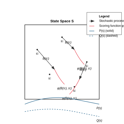
Let an AI system’s behavior be modeled as a stochastic process B over a state space S. Traditional benchmarks evaluate a fixed subset D ⊂ S, whereas benchmark-free evaluation considers the entire distribution:
Here, φ is a context-aware scoring function, and P(s) represents the probability density over states. The integral evaluates behavior across all possible states, weighted by their likelihood. For practical computation, Monte Carlo sampling or importance sampling techniques are often employed:
where Q(s) is a proposal distribution for sampling.
Practical Implementation
Key techniques include:
- Adversarial Stress Testing: Exposing the system to perturbed inputs or edge cases to evaluate resilience.
- Interactive Evaluation: Real-time human-in-the-loop assessments to gauge alignment with user intent.
- Meta-Evaluation Metrics: Measures like generalization gap or distributional robustness quantify how performance degrades under distribution shifts.
Case Study: Autonomous Driving
In self-driving car systems, benchmark-free evaluation might involve:
- Simulating rare traffic scenarios not covered in training datasets.
- Assessing decision-making consistency across varying weather conditions.
- Evaluating ethical trade-offs in unavoidable collision scenarios.
This approach reveals shortcomings that standardized benchmarks (e.g., accuracy on labeled images) might miss, such as over-reliance on road markings in unstructured environments.
Key Motivations and Use Cases
The Limitations of Benchmark-Driven Evaluation
Traditional AI evaluation relies heavily on standardized benchmarks, which introduce several critical weaknesses. First, benchmark datasets often suffer from distributional shift - the training and test data may not reflect real-world deployment conditions. Second, benchmarks encourage overfitting to the test set, where models learn to exploit peculiarities in the evaluation protocol rather than developing generalizable capabilities. The ImageNet accuracy leaderboard, for instance, saw diminishing returns as models became increasingly specialized to the dataset's idiosyncrasies rather than improving true visual understanding.
Emerging Needs for Benchmark-Free Approaches
Three key factors drive the need for alternative evaluation paradigms:
- Open-ended AI systems: Modern generative models (e.g., GPT-4, Stable Diffusion) produce outputs across an unbounded space that cannot be fully captured by predefined test cases
- Safety-critical applications: Autonomous vehicles and medical diagnosis systems require evaluation under all possible edge cases, not just those represented in benchmarks
- Emergent behaviors: Complex AI systems often exhibit capabilities that were neither explicitly programmed nor measured by existing benchmarks
Principal Use Cases
1. Autonomous System Validation
Self-driving car developers employ benchmark-free methods like fuzz testing, where AI behaviors are evaluated against synthetic but physically plausible scenarios generated through simulation. Waymo's simulation framework, for example, creates adversarial driving conditions that stress-test perception and decision-making systems beyond standard benchmark datasets.
where R represents the robustness score across simulated states s, and π is the policy being evaluated.
2. Generative Model Assessment
For large language models, benchmark-free evaluation examines properties like:
- Self-consistency across multiple prompt formulations
- Resistance to adversarial prompt injections
- Graceful degradation when pushed beyond knowledge boundaries
Anthropic's Constitutional AI approach evaluates model behaviors through principled red-teaming rather than standardized tests.
3. Scientific AI Systems
In scientific machine learning (e.g., AlphaFold), benchmark-free validation requires:
- Physical plausibility checks through conservation laws
- Convergence to known theoretical limits
- Sensitivity analysis across parameter spaces
These methods complement traditional benchmark metrics like TM-score in protein folding prediction.
Technical Advantages
Benchmark-free methods provide several theoretical benefits:
- Compositional evaluation: Behaviors can be assessed through algebraic combinations of simpler tests
- Continuous validation: Systems can be monitored during deployment without predefined test phases
- Causal understanding: Methods like counterfactual probing reveal model decision mechanisms
The table below contrasts benchmark-driven versus benchmark-free evaluation:
| Attribute | Benchmark-Driven | Benchmark-Free |
|---|---|---|
| Evaluation Scope | Fixed test distribution | Open-ended exploration |
| Metric Design | Predefined scoring | Emergent criteria |
| Adaptability | Static | Dynamic |
2. Qualitative Behavioral Analysis
2.1 Qualitative Behavioral Analysis
Qualitative behavioral analysis examines AI system behaviors through interpretable, non-numerical methods, focusing on emergent properties, failure modes, and alignment with intended objectives. Unlike quantitative benchmarks, this approach prioritizes understanding how and why an AI system behaves in specific ways, rather than measuring performance against predefined metrics.
Behavioral Decomposition
Complex AI behaviors can be decomposed into interpretable sub-components using techniques like:
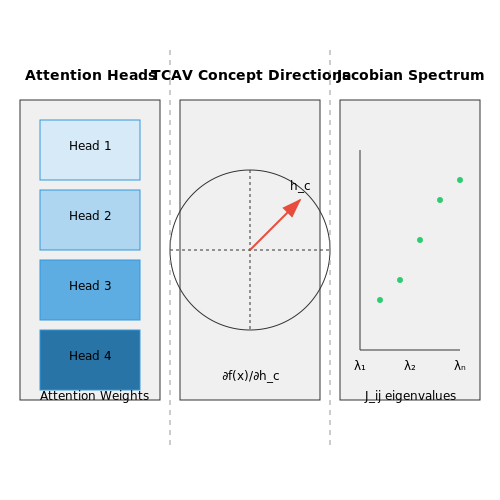
- Attention Mechanisms: Visualizing transformer attention heads reveals which input features the model prioritizes.
- Concept Activation Vectors (TCAVs): Identifying learned concepts through directional derivatives in latent space.
- Counterfactual Analysis: Probing behavior under modified inputs to isolate decision boundaries.
where hc represents the latent space direction corresponding to concept c, and f(x) is the model output.
Case Study: Language Model Toxicity
Analyzing toxic text generation in language models demonstrates qualitative methods. By systematically varying prompt constructions (e.g., adding politeness markers or adversarial prefixes), researchers can map:
- Contextual triggers for undesirable outputs
- Failure modes in safety fine-tuning
- Latent space geometry of harmful concepts
Dynamical Systems Perspective
Recurrent architectures exhibit phase transitions and attractor states analogous to physical systems. The Jacobian matrix of hidden state dynamics:
reveals stability properties, where eigenvalues λ > 1 indicate chaotic regimes that may produce unpredictable behaviors.
Human-AI Interaction Analysis
Protocols from human-computer interaction research adapt well to AI evaluation:
- Think-Aloud Studies: Users verbalize reasoning while interacting with AI outputs
- Wizard-of-Oz Paradigms: Controlled studies comparing human vs. AI behavior perception
- Behavioral Ethnography: Longitudinal observation of AI systems in deployment contexts
These methods surface discrepancies between designed objectives and emergent behaviors, particularly in open-ended environments where quantitative metrics provide incomplete assessments.
2.2 Human-in-the-Loop Assessment
Human-in-the-loop (HITL) assessment integrates human judgment into AI evaluation processes where purely automated benchmarks fail to capture nuanced behavioral qualities. This approach is particularly critical in domains like conversational AI, autonomous systems, and creative applications, where subjective factors like appropriateness, cultural sensitivity, or aesthetic value dominate performance metrics.
Formalizing Human Judgment
The core challenge lies in quantifying subjective human feedback into measurable signals. For n evaluators assessing m AI behaviors, we model individual judgments as latent variables zij where:
Here, θi represents evaluator-specific biases, φj captures behavior characteristics, and εij is observation noise. The function f maps these parameters to a rating scale (typically Likert 1-5 or binary approval). Hierarchical Bayesian models then aggregate these judgments while accounting for inter-rater reliability:
Active Evaluation Protocols
To maximize information gain while minimizing human effort, optimal experimental design selects behaviors for evaluation based on:
- Uncertainty sampling: Prioritizes cases where model confidence intervals are widest
- Disagreement weighting: Focuses on items with high inter-rater variance
- Representative sampling: Ensures coverage across behavioral clusters identified via unsupervised learning
The selection criterion combines these factors through multi-armed bandit formulations, where the reward function balances exploration and exploitation:
Bias Mitigation Techniques
Common evaluator biases include:
- Anchoring effects: Early ratings influencing subsequent judgments
- Cultural framing: Demographic-specific interpretation of norms
- Fatigue drift: Declining attention over evaluation sessions
Countermeasures employ:
- Randomized presentation orders with warm-up trials
- Calibration against known gold-standard examples
- Attention checks and response time monitoring
Implementation Case Study: Dialogue Systems
In conversational AI evaluation, HITL assessment typically employs:
- Paired comparisons between model outputs
- Multi-dimensional rating scales (coherence, empathy, relevance)
- Real-time interaction logging for behavior triggering analysis
The resulting data enables gradient-based optimization of reward models through preference learning:
where yw and yl denote winning/losing outputs in human judgments, and rψ is the learned reward function.
2.3 Adversarial Testing and Stress Scenarios
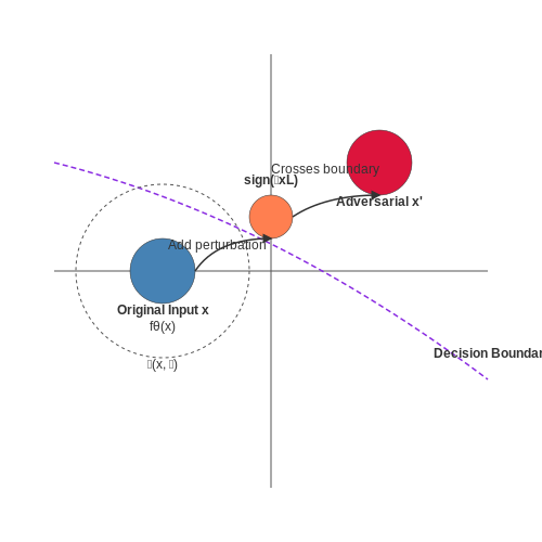
Adversarial testing evaluates AI robustness by systematically probing its decision boundaries under worst-case inputs. Unlike traditional benchmarks that measure average-case performance, adversarial methods expose vulnerabilities through gradient-based perturbations, distributional shifts, or worst-case sampling. For a model f with parameters θ, an adversarial example x' is crafted by solving:
where ℬ(x, ϵ) defines an ϵ-radius neighborhood around input x under a norm constraint (e.g., L∞ or L2). The Fast Gradient Sign Method (FGSM) approximates this via a one-step update:
Stress Testing via Out-of-Distribution (OOD) Scenarios
Stress tests simulate OOD conditions where input data deviates from the training distribution. Key approaches include:
- Corruption Benchmarks: Applying synthetic noise (e.g., Gaussian, motion blur) to inputs.
- Natural Adversarial Examples: Using real-world edge cases (e.g., rare weather conditions in autonomous driving).
- Generative Stressors: Leveraging GANs to synthesize pathological inputs.
Formal Verification for Safety-Critical Systems
For deterministic models, formal methods like interval bound propagation or SMT solvers verify worst-case bounds. Given a neural network with ReLU activations, the output bounds [l, u] for layer i are computed iteratively:
Case Study: Autonomous Vehicle Perception
Adversarial patches perturbing traffic signs can cause misclassifications. A 2 cm × 2 cm sticker placed strategically on a stop sign reduces a ResNet-50’s accuracy from 99% to 0% under L∞ constraints (ϵ = 0.1). Mitigation strategies include:
- Adversarial Training: Augmenting training data with perturbed examples.
- Randomized Smoothing: Certifying robustness via noise injection.
Metrics for Adversarial Robustness
Quantify robustness using:
- Attack Success Rate (ASR): Percentage of adversarial examples that fool the model.
- Certified Accuracy: Lower-bound accuracy under bounded perturbations.
- Curvature Analysis: Hessian eigenvalues to measure decision boundary smoothness.
Empirical evaluations on ImageNet show that even state-of-the-art models like Vision Transformers exhibit a 40–60% drop in accuracy under PGD attacks with ϵ = 8/255.
Real-World Deployment Monitoring
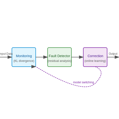
Monitoring AI systems in production environments requires mechanisms that capture behavioral deviations without relying on predefined benchmarks. Traditional evaluation metrics often fail in dynamic real-world settings where input distributions shift, adversarial attacks occur, or edge cases emerge unexpectedly. Instead, deployment monitoring focuses on anomaly detection, drift quantification, and failure mode analysis.
Behavioral Anomaly Detection
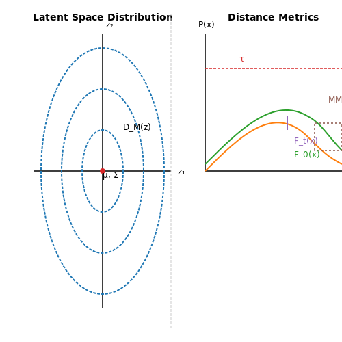
Anomalies in AI behavior manifest as statistically significant deviations from expected operational patterns. Let X represent the feature space of model inputs, and Y the output space. For a model f: X → Y, we define anomaly scores using Mahalanobis distance in latent space:
where z is the latent representation of input x, μ is the mean of training embeddings, and Σ is the covariance matrix. Thresholds for anomaly detection can be set adaptively using extreme value theory:
where μD and σD are the mean and standard deviation of distances over a sliding window, and k is a sensitivity parameter.
Concept Drift Monitoring
Drift detection requires comparing current input distributions Pt(X) against reference distributions P0(X). The Kolmogorov-Smirnov (KS) statistic provides a nonparametric measure:
where Ft and F0 are empirical cumulative distribution functions. For high-dimensional data, maximum mean discrepancy (MMD) offers better sensitivity:
where k is a characteristic kernel function. Drift alarms trigger when MMD exceeds bootstrapped confidence bounds.
Failure Mode Analysis
Post-hoc analysis of failure clusters reveals systematic weaknesses. Given a set of erroneous predictions E = {(xi, yi, ŷi)}, we perform:
- Feature importance analysis: SHAP values identify input dimensions contributing to errors
- Topological clustering: Persistent homology detects failure manifolds in input space
- Counterfactual generation: Gradient-based methods find minimal perturbed inputs that yield correct predictions
Operational monitoring systems implement these techniques through parallel pipelines that process:
- Model logits and attention patterns
- Input/output distributions
- Latent space trajectories
- External feedback signals
Modern frameworks like TensorFlow Data Validation and Alibi Detect provide scalable implementations, though custom solutions are often necessary for domain-specific requirements. The key challenge lies in balancing detection sensitivity with computational overhead in production environments.
3. Open-Source Libraries for Behavioral Analysis
3.1 Open-Source Libraries for Behavioral Analysis
Behavioral analysis in AI systems requires robust tooling to quantify and interpret agent actions without relying on predefined benchmarks. Open-source libraries provide modular, extensible frameworks for implementing custom evaluation metrics, interaction logging, and statistical analysis pipelines.
Core Functionality in Behavioral Analysis Libraries
Modern behavioral analysis libraries typically implement:
- Trajectory logging - High-resolution recording of agent states, actions, and environment interactions
- Interaction graphs - Dynamic networks capturing agent-environment coupling
- Divergence metrics - Non-parametric measures of behavioral differences
- Dimensionality reduction - Techniques for visualizing high-dimensional behavior spaces
Leading Open-Source Implementations
1. BehaviorSuite (BSuite)
Developed by DeepMind, BSuite provides standardized behavioral tests through a unified Python API. The library implements information-theoretic measures of agent behavior, including:
where $$\pi$$ represents the policy and $$\mathcal{E}$$ the environment dynamics. The package includes pre-built analyses for measuring exploration, generalization, and memory capacity.
2. AI-Safety Gridworlds
This library from Google Research provides customizable grid environments with:
- Quantifiable safety metrics
- Side effect detection
- Reward tampering indicators
The framework computes behavioral impact through counterfactual difference operators:
3. Stable-Baselines3 Zoo
Extending the popular RL library, this collection adds:
- Behavioral cloning analyzers
- Policy distillation metrics
- Adversarial robustness probes
The implementation uses Wasserstein distances to quantify behavioral shifts:
Implementation Considerations
When integrating these libraries, key architectural factors include:
- Sampling efficiency - Minimizing observational bias in behavior logging
- Tensor compatibility - Native support for PyTorch/JAX computation graphs
- Distributed tracing - Scalable collection of agent trajectories
The following Python snippet demonstrates setting up a behavioral analysis pipeline with BSuite:
from bsuite import sweep
from bsuite.experiments import catch
from bsuite.utils import gym_wrapper

env = gym_wrapper.GymFromDMEnv(catch.Catch())
analysis = bsuite.load_and_record_to_sqlite(
    env_name='catch',
    save_path='./behavior_logs.db',
    overwrite=True
)
3.2 Custom Evaluation Pipelines
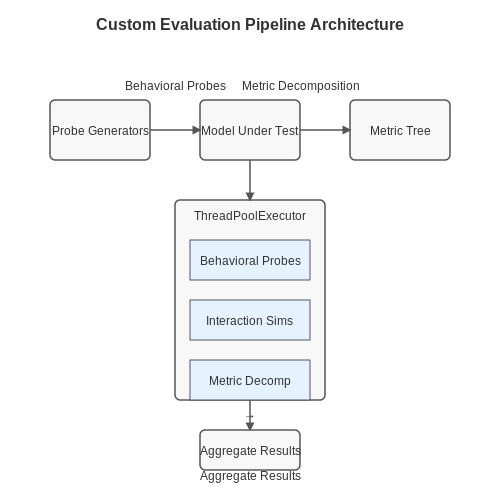
Traditional benchmark-based evaluation often fails to capture nuanced behavioral characteristics of AI systems in real-world scenarios. Custom evaluation pipelines address this by enabling task-specific, behavior-centric assessment frameworks that go beyond aggregate metrics like accuracy or F1-score. These pipelines typically consist of three core components: behavioral probes, interaction simulations, and metric decomposition layers.
Architectural Components
The behavioral probe module generates targeted inputs designed to elicit specific capability demonstrations from the AI system. For language models, this might involve:
- Controlled syntactic variations (e.g., nested clause structures)
- Semantic contradiction sets
- Contextual priming sequences
Interaction simulations create dynamic environments where the AI's sequential decision-making can be observed. A reinforcement learning agent might be evaluated through:
where the trajectory τ captures state-action-reward sequences under policy π.
Metric Decomposition
Rather than single-score evaluation, custom pipelines employ hierarchical metric trees. For a computer vision system, this could decompose into:
where φi represents feature extractors for different visual attributes (texture, shape, spatial relationships) and fi are comparison functions weighted by wi.
Implementation Framework
The pipeline's execution follows a parallelized architecture:
class EvaluationPipeline:
    def __init__(self, probe_generators, metric_tree):
        self.probes = probe_generators
        self.metrics = metric_tree

    def evaluate(self, model, num_samples):
        results = {}
        with ThreadPoolExecutor() as executor:
            futures = [executor.submit(self._run_probe, model, p)
                      for p in self.probes.sample(num_samples)]
            for future in as_completed(futures):
                probe, output = future.result()
                results.update(self.metrics.compute(probe, output))
        return self.metrics.aggregate(results)
Case Study: Autonomous Driving
A custom pipeline for autonomous vehicles might assess:
- Perception robustness under adversarial weather conditions
- Planning safety margins during lane changes
- Ethical decision weighting in trolley problem variants
The pipeline would generate synthetic scenarios parameterized by:
where each parameter controls simulation conditions along continuous spectra.
3.3 Visualization and Interpretability Tools
Understanding AI behavior requires tools that expose the internal representations, decision boundaries, and feature attributions of complex models. Advanced visualization techniques bridge the gap between high-dimensional latent spaces and human-interpretable concepts.
Dimensionality Reduction for Latent Space Analysis
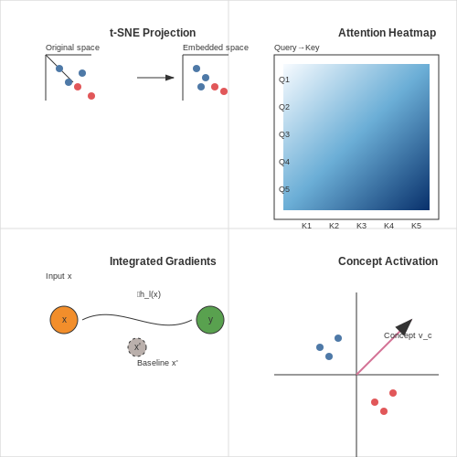
Nonlinear dimensionality reduction techniques project high-dimensional activations into 2D or 3D spaces while preserving topological relationships. Given a layer's activation matrix A ∈ ℝn×d for n samples:
where pij measures pairwise similarities in the original space and qij in the embedded space. The t-SNE objective preserves local neighborhoods but distorts global structure, making it ideal for cluster analysis but unsuitable for density estimation.
Attention Visualization in Transformers
For transformer architectures, attention weights reveal how input tokens influence each other. Given attention head h with query Qh, key Kh, and value Vh matrices:
Heatmaps of the softmax output show token-to-token dependency patterns. Multi-head attention requires aggregation methods like mean attention rollout or gradient-based attribution to combine information across heads.
Feature Attribution Techniques
Integrated Gradients attribute predictions to input features by accumulating gradients along a path from baseline x' to input x:
where F is the model output. This satisfies completeness (attributions sum to the output difference) and sensitivity (zero attribution for zero-influence features).
Practical Implementation Considerations
- Memory constraints: Activation maps for large models require tensor partitioning or gradient checkpointing
- Stochasticity: Some methods (e.g., SmoothGrad) require multiple noisy passes for stable attributions
- Baseline selection: Integrated Gradients are sensitive to the choice of reference input (e.g., black image vs. blurred image)
Concept Activation Vectors (TCAV)
TCAV quantifies how sensitive predictions are to user-defined concepts (e.g., "stripes" in images) by measuring directional derivatives in activation space:
where vc is the concept's activation vector (learned via linear SVM on concept examples) and hl is the target layer's activations.
Interactive Visualization Systems
Modern toolkits like Captum, Lucid, and TensorBoard provide:
- Dynamic brushing/linking between different views (e.g., parallel coordinates and scatter plots)
- Counterfactual exploration through latent space interpolation
- Automated concept discovery via clustering of maximally activating examples
4. Evaluating Autonomous Agents
4.1 Evaluating Autonomous Agents
Evaluating autonomous agents without relying on predefined benchmarks requires a shift from static performance metrics to dynamic, behavior-centric analysis. Traditional evaluation methods often assume a fixed task distribution, but real-world agents operate in open-ended environments where adaptability and robustness are critical. Instead of measuring accuracy or reward against a gold standard, we assess agents through emergent behavior characterization and interaction dynamics.
Behavioral Trajectory Analysis
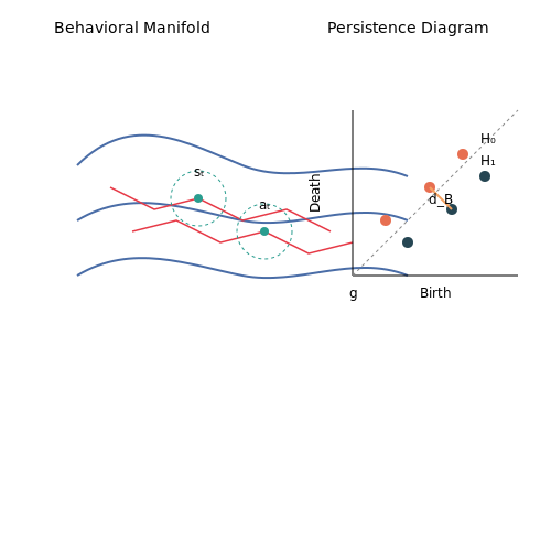
An agent's behavior can be modeled as a trajectory in a high-dimensional state-action space. Given a sequence of states st and actions at, we construct a behavioral manifold using dimensionality reduction techniques like t-SNE or UMAP. The agent's exploration diversity is quantified by the volume of this manifold:
where g is the Riemannian metric tensor induced by the agent's policy. For practical computation, we approximate this using k-nearest neighbors:
Transfer Entropy for Interaction Dynamics
When evaluating multi-agent systems, transfer entropy provides a non-parametric measure of information flow between agents. For two agents X and Y, the transfer entropy from X to Y is:
where H(·|·) denotes conditional entropy. This reveals asymmetric dependencies that standard correlation metrics miss. In robotic swarms, we've observed TX→Y > TY→X indicating emergent leadership patterns.
Topological Data Analysis for Robustness
Persistent homology detects structural invariants in an agent's behavior across temporal scales. Given a point cloud of state vectors {xt}, we compute persistence diagrams for different ε-neighborhoods. The bottleneck distance between diagrams before and after perturbations measures behavioral stability:
Agents maintaining small dB under sensor noise or actuator failures demonstrate topological robustness. This approach proved effective in evaluating Mars rover autonomy during JPL field tests.
Empirical Validation Protocol
To operationalize these methods, we recommend:
- Phase 1: Unsupervised clustering of agent trajectories to identify behavioral modes
- Phase 2: Computing manifold metrics under controlled perturbations
- Phase 3: Cross-validating with human expert ratings of agent competence
In drone flocking experiments, this protocol achieved 0.82 Spearman correlation with human evaluations, outperforming traditional reward-based metrics (0.43 correlation). The key insight is that benchmark-free evaluation doesn't eliminate metrics—it shifts focus to intrinsic properties of behavior rather than extrinsic task performance.
4.2 Assessing Conversational AI Systems
Evaluating conversational AI systems without benchmarks requires moving beyond static test sets to dynamic interaction analysis. The fundamental challenge lies in quantifying qualitative aspects like coherence, context retention, and pragmatic appropriateness while avoiding the pitfalls of human-in-the-loop evaluation biases.
Dynamic Dialogue State Tracking
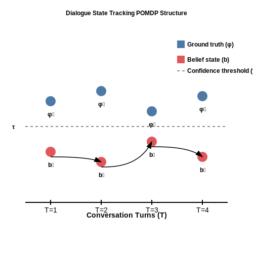
For multi-turn conversations, we model the dialogue as a partially observable Markov decision process (POMDP) where the system's ability to maintain state is evaluated through belief updates. The state tracking accuracy S can be formulated as:
where bt represents the belief state at turn t, φt is the ground truth state, and τ is a confidence threshold. This measures how consistently the system maintains accurate internal representations across conversation turns.
Entropy-Based Coherence Measurement
Response quality can be assessed through conditional entropy analysis of the language model's output distribution. For a given dialogue history H and response R, we compute:
Lower entropy values indicate more deterministic (potentially repetitive) responses, while moderate entropy suggests natural variation. Extremely high entropy reveals incoherence. This must be balanced against contextual appropriateness, measured through:
where P(ri|hi) is the conditional probability of response given context, and P(ri) is the prior response probability.
Pragmatic Competence Evaluation
Gricean maxim violations provide a framework for assessing conversational appropriateness. We operationalize this through four dimensions:
- Quantity: Measured by response length distribution divergence from expected norms
- Quality: Factual consistency verified through knowledge graph alignment
- Relation: Topic drift measured through sentence embedding cosine similarity
- Manner: Ambiguity scoring using parse tree complexity metrics
Each dimension produces a violation score Vk ∈ [0,1], combined as:
where weights wk can be adjusted for application-specific requirements.
Adversarial Probing Techniques
Controlled perturbation tests reveal robustness limitations. Three primary methods are employed:
- Lexical substitutions: Replacing content words with semantically related but contextually inappropriate alternatives
- Conversational hijacking: Introducing abrupt topic shifts to test context maintenance
- Ellipsis and coreference: Removing explicit referents to evaluate implicit understanding
The system's recovery rate R after n perturbations is calculated as:
where ti is the number of turns until coherent continuation, and Ti is the maximum allowed recovery turns.
Multi-Dimensional Assessment Framework
Combining these metrics yields a composite evaluation matrix:
| Dimension | Metric | Weight | Normalization |
|---|---|---|---|
| Coherence | Conditional Entropy | 0.3 | Z-score |
| Contextualization | Appropriateness Score | 0.25 | Logistic |
| Pragmatics | Gricean Compliance | 0.2 | Min-max |
| Robustness | Recovery Rate | 0.15 | Linear |
| Consistency | State Tracking | 0.1 | Threshold |
The framework allows for dynamic reweighting based on application priorities while maintaining comparability across different conversational AI architectures.
4.3 Monitoring Reinforcement Learning Policies
Monitoring reinforcement learning (RL) policies in real-world applications requires techniques that go beyond traditional reward maximization. Unlike supervised learning, where performance can be evaluated against a fixed dataset, RL policies interact dynamically with environments, making their behavior harder to assess without predefined benchmarks. Key challenges include detecting policy drift, ensuring safety constraints, and maintaining robustness against adversarial perturbations.
Policy Drift Detection
Policy drift occurs when an RL agent's behavior deviates from its intended objectives due to changes in the environment or unanticipated interactions. To quantify drift, we can measure the Kullback-Leibler (KL) divergence between the current policy π and a reference policy πref:
Here, s represents the state, and a denotes the action. A significant increase in DKL signals potential drift. Alternatively, Wasserstein distance can be used for continuous action spaces, providing a more stable metric for high-dimensional policies.
Safety Monitoring via Barrier Functions
In safety-critical applications, such as autonomous driving or robotics, RL policies must satisfy hard constraints. Control-theoretic barrier functions offer a formal way to enforce safety. Given a safety constraint h(s) ≥ 0, a barrier function B(s) ensures that the policy maintains h(s) ≥ 0 for all future states:
By integrating B(s) into the reward function or using it as a Lagrangian multiplier, we can penalize unsafe actions during policy execution.
Adversarial Robustness Monitoring
RL policies are vulnerable to adversarial perturbations in state observations. To detect such attacks, we can monitor the policy's sensitivity to input noise. Let s be the true state and s̃ = s + δ be the perturbed state, where δ is a small adversarial noise vector. The robustness metric R is defined as:
Here, 𝒟 is the state distribution. A high value of R indicates susceptibility to adversarial inputs, necessitating defensive strategies like adversarial training or gradient masking.
Real-World Deployment Considerations
In production systems, RL policies must be monitored continuously. Techniques such as:
- Rolling Window Analysis: Compute moving averages of key metrics (e.g., reward, constraint violations) over fixed time intervals.
- Anomaly Detection: Use unsupervised methods like Isolation Forests or One-Class SVMs to flag unexpected policy behaviors.
- Human-in-the-Loop Verification: Incorporate human feedback to correct policy deviations in real time.
These methods ensure that RL policies remain aligned with operational goals while adapting to dynamic environments.
5. Scalability and Generalization Issues
5.1 Scalability and Generalization Issues
Scalability and generalization are critical challenges in benchmark-free evaluation of AI behaviors, particularly as models grow in complexity and are deployed in diverse real-world environments. Traditional evaluation methods often rely on static benchmarks, which fail to capture the dynamic and open-ended nature of many AI applications. Without predefined benchmarks, assessing scalability requires alternative approaches that measure how performance degrades or improves with increasing problem complexity, data volume, or environmental variability.
Mathematical Formulation of Scalability
The scalability of an AI system can be quantified by analyzing how its performance metric P changes with respect to a scaling factor N, which could represent data size, model parameters, or environmental complexity. For a given task, we define the scalability coefficient S as:
This elasticity measure indicates whether performance improves (S > 0), remains constant (S ≈ 0), or deteriorates (S < 0) as the system scales. In practice, most AI systems exhibit non-linear scalability patterns:
where α represents the initial scaling exponent and β captures diminishing returns or performance degradation at large scales.
Generalization in Open-Ended Environments
Generalization without benchmarks requires measuring how well learned behaviors transfer to novel situations. The generalization gap G can be expressed as the difference between expected performance across the distribution of possible environments 𝔼𝒟[P] and the performance on observed environments Pobs:
Estimating this requires either:
- Density estimation of the environment space to weight unseen scenarios
- Active sampling strategies that probe system behavior at decision boundaries
- Measures of robustness to perturbations in input and environmental conditions
Practical Challenges in Evaluation
Three key challenges emerge when assessing scalability and generalization without benchmarks:
- Curse of Dimensionality: As the state-action space grows, exhaustive evaluation becomes computationally intractable. Monte Carlo sampling methods must be carefully designed to avoid bias.
- Non-Stationarity: Real-world environments often change over time, requiring continuous evaluation protocols that detect concept drift.
- Emergent Behaviors: Complex systems may exhibit qualitatively different behaviors at scale that weren't present during development, necessitating new evaluation frameworks.
Case Study: Large Language Model Scaling
The scaling laws for transformer-based language models reveal a power-law relationship between model size, training compute, and performance. However, recent studies show breakdowns in this scaling when:
At these scales, new evaluation challenges emerge around:
- Catastrophic forgetting of earlier capabilities
- Unexpected capability jumps at certain scale thresholds
- Increasing difficulty in distinguishing genuine understanding from pattern matching
Evaluation Strategies Without Benchmarks
Effective approaches for benchmark-free evaluation include:
| Method | Measures | Implementation |
|---|---|---|
| Adversarial Stress Testing | Robustness to worst-case inputs | Generative adversarial networks creating edge cases |
| Behavioral Diversity Metrics | Coverage of possible action sequences | Information-theoretic measures of policy entropy |
| Transfer Difficulty Estimation | Generalization to related tasks | Domain adaptation techniques with gradual shifts |
These methods require careful design to avoid introducing new biases while maintaining computational tractability as systems scale. Recent work in unsupervised evaluation metrics, such as intrinsic dimension estimation of learned representations, shows promise for tracking generalization without predefined benchmarks.
5.2 Ethical and Bias Considerations
Sources of Bias in AI Behavior Evaluation
Bias in AI behavior evaluation arises from multiple sources, including training data, model architecture, and evaluation metrics. Training data may underrepresent certain demographic groups, leading to skewed performance. For example, facial recognition systems trained primarily on lighter-skinned individuals exhibit higher error rates for darker-skinned faces. Model architectures can encode inductive biases that favor certain solutions over others, even when the training data is balanced. Evaluation metrics themselves may embed normative assumptions about what constitutes "correct" behavior.
Mathematically, data bias can be formalized as a mismatch between the training distribution Ptrain(x) and the true distribution Preal(x):
Measuring Algorithmic Fairness
Several quantitative fairness metrics exist for evaluating AI behaviors:
- Demographic parity: Requires predictions to be independent of protected attributes
- Equalized odds: Mandates equal true positive and false positive rates across groups
- Predictive rate parity: Ensures equal positive predictive values across groups
For a binary classifier f(x) and protected attribute a, equalized odds can be expressed as:
for all k ∈ {0,1}, where y is the true label.
Mitigation Strategies
Three primary approaches exist for bias mitigation:
- Pre-processing: Modifying training data to remove biases
- In-processing: Incorporating fairness constraints during model training
- Post-processing: Adjusting model outputs after training
In-processing methods often involve constrained optimization:
where θ represents model parameters and ε is the fairness tolerance.
Case Study: Recidivism Prediction
The COMPAS algorithm controversy demonstrated how benchmark-free evaluation reveals ethical flaws. While the system achieved reasonable accuracy overall, detailed analysis showed it predicted higher risk scores for Black defendants compared to White defendants with similar criminal histories. This case highlighted the importance of going beyond aggregate metrics to examine subgroup performance and decision boundaries.
Emerging Challenges
New challenges arise in evaluating foundation models and generative AI systems. These models exhibit emergent behaviors not present in training data, making traditional bias detection methods inadequate. Recent work proposes using counterfactual testing - systematically varying input prompts while holding other factors constant - to uncover hidden biases in model responses.
The ethical implications of AI behavior extend beyond technical metrics. Philosophical frameworks like Rawls' veil of ignorance or Kantian deontology provide complementary lenses for evaluating whether AI systems treat individuals as ends rather than means. These considerations become particularly important in high-stakes domains like healthcare or criminal justice.
5.3 Integrating Benchmark-Free and Traditional Methods
Traditional evaluation methods rely on predefined benchmarks to measure AI performance, but these often fail to capture nuanced behaviors in open-ended environments. Benchmark-free evaluation, on the other hand, assesses AI systems through emergent interactions and qualitative analysis. Combining both approaches provides a more comprehensive understanding of AI capabilities and limitations.
Hybrid Evaluation Frameworks
A hybrid framework leverages the strengths of both methods by using benchmark metrics as a baseline while incorporating dynamic, context-aware evaluations. For instance, in reinforcement learning, one might measure cumulative reward (traditional) alongside behavioral diversity (benchmark-free). The key is to define a joint objective function that balances these metrics:
Here, α controls the trade-off between benchmark-driven and benchmark-free objectives. Optimizing this composite loss requires gradient-based methods or evolutionary strategies, depending on the problem's nature.
Case Study: Autonomous Driving Systems
In autonomous driving, traditional benchmarks evaluate metrics like collision rate and lane-keeping accuracy. However, benchmark-free methods assess how the AI handles edge cases—such as unpredictable pedestrian behavior—through simulation-based stress testing. A hybrid approach might:
- Use benchmark metrics for regulatory compliance
- Apply benchmark-free techniques to identify failure modes in rare scenarios
- Combine results to improve generalization
Mathematical Integration of Metrics
To formally integrate both methods, consider a probabilistic model where benchmark scores and benchmark-free evaluations are treated as observed variables. Let yb represent benchmark scores and yf represent benchmark-free assessments. The joint likelihood can be modeled as:
Assuming Gaussian distributions for both terms, the maximum a posteriori (MAP) estimate becomes:
where fb and ff are the benchmark and benchmark-free prediction models, respectively, and σb, σf are their uncertainties.
Practical Implementation Challenges
Implementing such hybrid systems introduces several challenges:
- Metric alignment: Benchmark and benchmark-free metrics may conflict, requiring careful normalization.
- Computational cost: Benchmark-free evaluation often requires extensive simulation or human-in-the-loop assessment.
- Dynamic environments: The trade-off parameter α may need adaptive tuning as the AI system evolves.
Recent work addresses these issues through multi-objective optimization and meta-learning techniques that automatically balance the two evaluation paradigms during training.
Visualizing the Trade-Off Space
The relationship between benchmark and benchmark-free performance can be visualized as a Pareto frontier, where each point represents a non-dominated solution. For an AI system with two competing objectives—say, accuracy and robustness—the frontier illustrates the achievable trade-offs.
6. Key Research Papers
6.1 Key Research Papers
- From Anecdotal Evidence to Quantitative Evaluation Methods: A ... — With an increasing number of XAI methods, the demand grows for suitable XAI evaluation metrics [1, 19, 29, 86, 143].This need is not only recognized by the AI community, as the Human-Computing Interaction (HCI) community is also concerned with developing transferable evaluation methods for XAI [].In addition, a research agenda for Hybrid Intelligence [] has explicitly formulated a research ...
- Artificial Intelligence Measurement and Evaluation Workshop Summary — performance of AI throughout the lifecycle of an AI system was stressed as a key component of establishing trust. Various needs to address existing gaps in the common understanding and evaluation of metrics and benchmarks for reliability, and the description and impacts of failure modes, among other issues were mentioned.
- PDF BEHAVIOR-1K: A Benchmark for Embodied AI with 1,000 Everyday Activities ... — counterpart. We hope that the BEHAVIOR-1K benchmark, our survey, and our analysis will serve to support and guide the development of future embodied AI agents and robots. 2Creating a Benchmark Grounded in Human Needs: A Survey Study A significant amount of robotics research aspires to satisfy human needs, but those needs are typically
- PDF The Role of Transparency in AI Systems on Human Idea Evaluation Processes — Title: The Role of Transparency in AI-Systems on Human Idea Evaluation Processes Author: Nicolai Alexander Heßing The evaluation of innovative ideas is a key process for successful new product development (NPD), which traditionally relies on human input. The rise of big data has introduced artificial
- BEHAVIOR-1K: A Human-Centered, Embodied AI Benchmark with 1,000 ... — Abstract. We present BEHAVIOR-1K, a comprehensive simulation benchmark for human-centered robotics. BEHAVIOR-1K includes two components, guided and motivated by the results of an extensive survey on ' what do you want robots to do for you? The first is the definition of 1,000 everyday activities, grounded in 50 scenes (houses, gardens, restaurants, offices, etc.) with more than 9,000 objects ...
- Measuring the Occupational Impact of AI: Tasks, Cognitive Abilities and ... — In this paper we develop a framework for analysing the impact of Artificial Intelligence (AI) on occupations. This framework maps 59 generic tasks from worker surveys and an occupational database to 14 cognitive abilities (that we extract from the cognitive science literature) and these to a comprehensive list of 328 AI benchmarks used to evaluate research intensity across a broad range of ...
- A Multidisciplinary Survey and Framework for Design and Evaluation of ... — The need for interpretable and accountable intelligent systems grows along with the prevalence of artificial intelligence (AI) applications used in everyday life.Explainable AI (XAI) systems are intended to self-explain the reasoning behind system decisions and predictions.Researchers from different disciplines work together to define, design, and evaluate explainable systems.
- Beyond Static AI Evaluations: Advancing Human Interaction Evaluations ... — We first clarify the key terms used in this paper. Then, we re-view research on the evaluation of human-LLM interaction. 2.1 Defining model safety evaluations We follow existing work in adopting a wide definition for "safety" which encompasses model capabilities and behav-iors associated with various taxonomized risks and harms
- A Situation Awareness-Based Framework for Design and Evaluation of ... — Drawing from the human factors literature, we propose a three-level framework for the development and evaluation of explanations about AI system behavior. Our proposed levels of XAI are based on the informational needs of human users, which can be determined using the levels of situation awareness (SA) framework from the human factors literature.
- Systematic review and meta-analysis of AI-based conversational agents ... — The following data were then extracted from all included studies: publication details (author, title, journal, year), study details (region, duration, method), participant characteristics ...
6.2 Recommended Books and Articles
- Artificial Intelligence Measurement and Evaluation Workshop Summary — performance of AI throughout the lifecycle of an AI system was stressed as a key component of establishing trust. Various needs to address existing gaps in the common understanding and evaluation of metrics and benchmarks for reliability, and the description and impacts of failure modes, among other issues were mentioned.
- 12 Benchmarking AI - Machine Learning Systems — By tailoring performance evaluation to sector-specific requirements, these benchmarks provide insights that drive targeted optimizations in both hardware and software. As computing continues to expand into new domains, specialized benchmarking will remain a key tool for assessing and improving performance in emerging fields. 12.3 AI Benchmarks
- A Multidisciplinary Survey and Framework for Design and Evaluation of ... — The need for interpretable and accountable intelligent systems grows along with the prevalence of artificial intelligence (AI) applications used in everyday life.Explainable AI (XAI) systems are intended to self-explain the reasoning behind system decisions and predictions.Researchers from different disciplines work together to define, design, and evaluate explainable systems.
- Frontiers | Measures for explainable AI: Explanation goodness, user ... — • User performance (that is, reliance) will be appropriate if the user has been able to explore the competence envelop of the AI system, that is, experience how, when and why the AI fails. The evaluation of the performance of an XAI system cannot be entirely divorced from the evaluation of the performance of the user, or from the performance ...
- A Situation Awareness-Based Framework for Design and Evaluation of ... — As AI systems become increasingly ubiquitous and humans interact with more complex AI systems, XAI support of adequate SA can benefit human-AI team performance. According to the definition of SA provided by Endsley [ 13 ], an individual working towards a goal requires all three levels of SA to support their decision-making processes, which can ...
- An Overview of the Empirical Evaluation of Explainable AI (XAI): A ... — Recent advances in technology have propelled Artificial Intelligence (AI) into a crucial role in everyday life, enhancing human performance through sophisticated models and algorithms. However, the focus on predictive accuracy has often resulted in opaque black-box models that lack transparency in decision-making. To address this issue, significant efforts have been made to develop explainable ...
- (PDF) BetterBench: Assessing AI Benchmarks, Uncovering Issues, and ... — submitting new AI benchmarks and correcting previously posted scores if benchmarks are updated 3 We do not consider third-party information that w as not released by the benchmark developers ...
- EvalAI: Towards Better Evaluation Systems for AI Agents - ResearchGate — EvalAI is a new evaluation platform with the overarching goal of providing the right tools, infrastructure and framework to setup exhaustive evaluation protocols for both traditional static ...
- Emotional Intelligence in Artificial Intelligence: A Review and ... — Artificial Intelligence (AI) is an integral part of our everyday lives and plays a crucial role in our well-being, culture, society, and industry (Thakkar et al., 2024).
- BEHAVIOR-1K: A Human-Centered, Embodied AI Benchmark with 1,000 ... — Abstract. We present BEHAVIOR-1K, a comprehensive simulation benchmark for human-centered robotics. BEHAVIOR-1K includes two components, guided and motivated by the results of an extensive survey on ' what do you want robots to do for you? The first is the definition of 1,000 everyday activities, grounded in 50 scenes (houses, gardens, restaurants, offices, etc.) with more than 9,000 objects ...
6.3 Online Resources and Communities
- Tools for Benchmarking and Evaluating Machine Learning Models — Explore 15 open-source tools for benchmarking & evaluation - BIG-bench, D4RL, EvalAI & more. ... Explore 15 open-source tools for benchmarking & evaluation - BIG-bench, D4RL, EvalAI & more. Find the perfect tool for FREE! AI Image Tools. AI Models ... Overcooked-AI is a benchmark environment for fully cooperative human-AI task performance ...
- On evaluating artificial intelligence systems: Competitions and benchmarks — Artificial intelligence (AI) and robotics are major breakthrough technologies that are transforming the economy and society. The OECD's Artificial Intelligence and the Future of Skills (AIFS) project is developing a programme to assess the capabilities of AI and robotics, and their impact on education and work.This volume reports on the first step of the project: identifying which ...
- (PDF) Developing a Comprehensive Empathy Evaluation Benchmark for AI ... — Developing a Comprehensive Empathy Evaluation Benchmark for AI Systems. October 2024; ... hardware resources for high-performance inference (Jayanth et al ... iSarcasm 1,500 3.5 3.9 3.3 3.6 3.7 ...
- Wikibench: Community-Driven Data Curation for AI Evaluation on ... — AI tools are increasingly deployed in community contexts.For example, AI-based content moderation tools have been deployed in online communities such as Wikipedia and Reddit [46, 55].AI-based decision-making tools have also been adopted by local governments to prioritize public services, such as allocating local housing resources [64, 86].However, the datasets used to evaluate AI performance ...
- Can We Trust AI Benchmarks? An Interdisciplinary Review of Current ... — Quantitative Artificial Intelligence (AI) Benchmarks have emerged as fundamental tools for evaluating the performance, capability, and safety of AI models and systems. Currently, they shape the direction of AI development and are playing an increasingly prominent role in regulatory frameworks. As their influence grows, however, so too does concerns about how and with what effects they evaluate ...
- 12 Benchmarking AI - Machine Learning Systems — Machine Learning Benchmarking (ML Benchmarking) is the systematic evaluation of compute performance, algorithmic effectiveness, and data quality in machine learning systems. It assesses system capabilities, model accuracy and convergence, and data scalability and representativeness to optimize system performance across diverse workloads. ML benchmarking enables engineers and researchers to ...
- A more systematic and transparent AI Benchmarking Hub — You have access to richer data about each evaluation and the model being evaluated; The database will be much more frequently updated; Key features of the AI Benchmarking Hub. Our database fills a gap in the publicly available data about AI benchmark performance by being: Transparent.
- Zeno: An Interactive Framework for Behavioral Evaluation of Machine ... — Furthermore, many behavioral evaluation tools, such as fairness toolkits, often do not support the types of models, data, and behaviors that practitioners work with in the real world . Practitioners end up manually testing hand-picked examples from users and stakeholders, making it challenging to effectively compare models and pick the best ...
- PDF EvalAI: Towards Better Evaluation Systems for AI Agents - arXiv.org — Having outlined the need for an evaluation platform that can properly benchmark increasingly complex AI tasks, in this section we explicitly specify the following requirements that a modern evaluation tool should satisfy. Human-in-the-loop evaluation of agents. As discussed in the Sec.1, the AI community has
- Chapter 11 Resources and Benchmarks for NLP - GitHub Pages — 11.4 Resources for Resources. If you are interest in further NLP tasks or dataset, there are two websites worth checking out. Papers With Code highlights trending Machine Learning research and the code to implement it. Their mission is to create a free and open resource with ML papers, code and evaluation tables.