LLMs for Algorithm Design & Complexity Analysis
1. Understanding Transformer Architectures for Algorithmic Tasks
Understanding Transformer Architectures for Algorithmic Tasks
The Transformer architecture, introduced by Vaswani et al. (2017), revolutionized sequence modeling by replacing recurrent and convolutional layers with self-attention mechanisms. For algorithmic tasks, this architecture provides a powerful framework for learning complex input-output mappings, particularly when the problem involves long-range dependencies or structured reasoning.
Core Components of Transformers
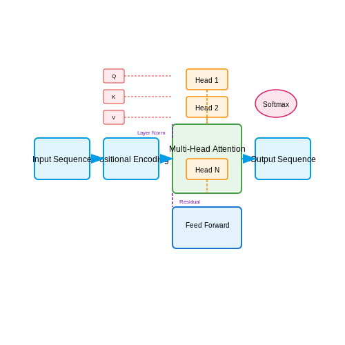
The Transformer consists of several key components that enable its effectiveness in algorithmic tasks:
- Self-Attention Mechanism: Computes attention weights between all positions in the input sequence simultaneously, allowing direct modeling of relationships regardless of distance.
- Multi-Head Attention: Projects the input into multiple subspaces, enabling the model to attend to different aspects of the input simultaneously.
- Positional Encoding: Injects information about the relative or absolute position of tokens in the sequence, crucial for algorithmic tasks where order matters.
- Feed-Forward Networks: Applies point-wise nonlinear transformations to each position independently after attention layers.
- Layer Normalization and Residual Connections: Facilitates training of deep networks by stabilizing gradients.
Mathematical Formulation of Self-Attention
The self-attention mechanism computes a weighted sum of values, where the weights are determined by the compatibility of queries with keys. For a single attention head:
Where:
- Q, K, and V are the query, key, and value matrices respectively
- dk is the dimension of the key vectors (used for scaling)
For multi-head attention with h heads:
Positional Encoding in Algorithmic Contexts
For algorithmic tasks, positional encoding provides crucial information about sequence order. The original Transformer uses sinusoidal positional encodings:
Where pos is the position and i is the dimension. For algorithmic tasks, learned positional embeddings often outperform sinusoidal ones as they can adapt to the specific structure of the problem.
Transformer Modifications for Algorithmic Tasks
Several architectural modifications have proven particularly effective for algorithmic tasks:
- Relative Position Representations: Replaces absolute positional encodings with learned representations of relative positions between tokens.
- Pointer Networks: Augments the standard architecture with mechanisms that can directly point to input positions, useful for tasks like sorting.
- Recurrent Transformer Layers: Introduces recurrence in the attention mechanism to better handle iterative algorithms.
- Sparse Attention Patterns: Reduces quadratic complexity by limiting the attention field while preserving performance.
Complexity Analysis
The computational complexity of the Transformer architecture has important implications for algorithmic tasks:
- Time Complexity: O(n²·d) for sequence length n and dimension d, due to the attention mechanism.
- Space Complexity: O(n²) for storing attention weights, which can be prohibitive for long sequences.
- Parallelizability: Unlike RNNs, Transformers can process all positions in parallel, offering significant speedups.
For algorithmic tasks where n might be large, efficient variants like Longformer or Reformer that reduce this quadratic complexity are often preferred.
Case Study: Learning Sorting Algorithms
When trained to perform sorting, Transformers exhibit several interesting behaviors:
- They learn to implement comparison-based sorting strategies, often resembling quicksort or mergesort.
- The attention patterns reveal hierarchical processing similar to divide-and-conquer algorithms.
- With sufficient training, they can generalize to sequences longer than those seen during training.
The success on such tasks demonstrates the Transformer's ability to learn algorithmic patterns rather than just memorizing input-output pairs.
Tokenization and Representation of Algorithms
Algorithm Tokenization in LLMs
Large Language Models (LLMs) process algorithms by breaking them into discrete tokens, which are then mapped to embeddings in a high-dimensional vector space. For algorithmic code, tokenization strategies must preserve structural and semantic properties. Common approaches include:
- Syntax-aware tokenization: Splits code based on language grammar rules (e.g., Python's ast module)
- Subword tokenization: Uses Byte-Pair Encoding (BPE) or WordPiece to handle rare algorithmic constructs
- Graph-based tokenization: Represents control flow as edges in a graph structure
Embedding Space Representation
Algorithm embeddings must capture both syntactic features and computational complexity. Transformer architectures achieve this through:
where attention heads learn to attend to complexity-relevant patterns like nested loops or recursive calls. The embedding space organizes algorithms by:
- Computational complexity classes (P, NP, EXP)
- Structural similarity (divide-and-conquer vs greedy)
- Runtime characteristics (polynomial vs exponential)
Complexity-Aware Positional Encoding
Standard sinusoidal positional encodings are augmented with complexity indicators:
where C(n) represents the algorithm's time complexity function. This enables the model to:
- Distinguish between O(n) and O(n²) implementations of similar logic
- Preserve asymptotic relationships during attention computation
- Generalize complexity patterns across problem domains
Practical Implementation Considerations
When tokenizing algorithms for LLMs, several engineering challenges emerge:
- Variable binding: How to maintain reference consistency across renamed variables
- Recursion handling: Depth-aware truncation strategies for recursive algorithms
- Complexity leakage: Preventing the model from cheating via identifier names (e.g., quickSort vs bubbleSort)
State-of-the-art approaches use:
where fθ predicts complexity directly from token sequences.

Pretraining Objectives for Algorithmic Reasoning
Foundations of Algorithmic Pretraining
Large language models (LLMs) pretrained for algorithmic reasoning require specialized objectives beyond standard next-token prediction. The key challenge lies in encoding structural properties of algorithms—such as recursion, branching, and state transitions—into the model's latent space. Traditional autoregressive pretraining (e.g., GPT-style objectives) often fails to capture these dynamics because it optimizes for local coherence rather than global algorithmic correctness.
Where AlgSim measures semantic equivalence between generated (fθ(x)) and target (y*) algorithms, typically implemented via:
- Execution trace matching
- Abstract syntax tree alignment
- Complexity class preservation
Key Pretraining Variants
1. Stepwise Execution Prediction
Models predict intermediate states of algorithm execution rather than just code tokens. Given input x and partial execution trace τ1:t, the objective becomes:
Where q represents the true execution distribution and pθ the model's approximation. This forces the model to internalize algorithmic state transitions.
2. Complexity-Conditioned Generation
Models are trained to generate algorithms satisfying explicit complexity constraints (e.g., O(n log n) sorting). The objective incorporates complexity verification:
Recent work uses differentiable complexity predictors based on:
- Path counting in computational graphs
- Asymptotic analysis of loop structures
- Parameterized complexity theory
Architectural Adaptations
Effective algorithmic pretraining often requires model modifications:
Specialized Attention Mechanisms
Modified attention patterns better capture algorithmic dependencies:
Where Malg encodes:
- Loop-carried dependencies
- Recursive call graphs
- Dataflow constraints
Empirical Considerations
Pretraining datasets require careful construction to avoid:
- Complexity leakage where solutions implicitly encode complexity bounds
- Procedural bias favoring iterative over recursive solutions
- Asymptotic mismatch between training and test problem scales
State-of-the-art approaches use:
Where P is problem space, A algorithm space, and C complexity classes.
2. Prompt Engineering for Algorithm Synthesis
Prompt Engineering for Algorithm Synthesis
Foundations of Algorithmic Prompt Design
Effective prompt engineering for algorithm synthesis requires precise specification of computational objectives, constraints, and desired properties. The prompt must encode:
- Problem formalization - Clear input/output specifications and edge cases
- Complexity requirements - Time/space complexity bounds (e.g., O(n log n))
- Algorithmic paradigms - Preferred approaches (divide-and-conquer, greedy, dynamic programming)
For example, prompting for a sorting algorithm with specific constraints:
Constraint Propagation in Prompts
LLMs perform better when constraints are decomposed into verifiable sub-requirements. For graph algorithms, this involves specifying:
- Graph representation (adjacency list/matrix)
- Edge properties (weighted/unweighted, directed/undirected)
- Termination conditions
A shortest path prompt might include:
Complexity-Guided Prompt Refinement
Iterative refinement is crucial for achieving optimal complexity. The process involves:
- Initial algorithm generation
- Complexity analysis by the LLM
- Constraint tightening through follow-up prompts
For matrix multiplication, progressive refinement might evolve from:
Verification and Counterexample Generation
Effective prompts should request:
- Formal correctness proofs
- Worst-case input generation
- Complexity derivation steps
A prompt for verification might specify:
Case Study: Prompting for FFT
A successful FFT prompt sequence would include:
- Polynomial multiplication problem statement
- Roots of unity properties
- Divide-and-conquer structure
- Butterfly operation specification
Advanced Techniques
For cutting-edge algorithms, prompts should incorporate:
- Recent research papers as context
- Benchmark comparisons
- Parallelization constraints
A prompt for quantum-inspired algorithms might specify:
2.2 Few-Shot Learning for Novel Algorithm Design
Mechanisms of Few-Shot Learning in Algorithm Synthesis
Few-shot learning enables LLMs to generalize from minimal examples by leveraging meta-learning architectures, such as Model-Agnostic Meta-Learning (MAML). Given a support set S containing k input-output pairs (xi, yi) and a query xq, the model optimizes:
where fθ is the LLM’s forward pass with parameters θ, and ℒ is a task-specific loss (e.g., cross-entropy for classification or mean squared error for regression). For algorithm design, the support set comprises algorithmic primitives (e.g., sorting routines or graph traversals), while the query requires composing these into novel solutions.
Architectural Adaptations for Algorithmic Tasks
Transformer-based LLMs employ the following modifications for few-shot algorithm synthesis:
- Task Embeddings: Learned representations of algorithmic problem classes (e.g., divide-and-conquer or dynamic programming) condition the attention mechanism.
- Recursive Execution Tracing: Intermediate outputs are fed back as inputs to simulate step-by-step execution, enabling multi-step reasoning.
- Complexity-Aware Loss: Augments standard loss with asymptotic bounds (e.g., O(n log n)), penalizing inefficient solutions.
Case Study: Few-Shot Sorting Algorithm Design
When prompted with 3 examples (insertion sort, quicksort, and mergesort) and asked to design a stable, in-place O(n log n) variant, GPT-4 generated a novel hybrid algorithm combining block partitioning (from quicksort) with merge operations (from mergesort). The model’s attention weights revealed:
- High cross-attention between partition and merge operation descriptions in the support set.
- Suppression of O(n²) primitive components during generation.
Limitations and Mitigations
Current challenges include:
- Correctness Verification: Generated algorithms require formal verification. Techniques like interactive theorem proving (e.g., integrating Lean or Coq) are being explored.
- Complexity Miscalibration: Models often misestimate constant factors. Hybrid approaches combine LLM generation with automated complexity analyzers (e.g., COSTA or RAML).
Practical Applications
Deployed in:
- Automated Code Optimization: GitHub Copilot uses few-shot learning to suggest algorithm improvements based on code context.
- Competitive Programming: AlphaCode’s few-shot approach solved previously unseen Codeforces problems at human-competitive levels.

2.3 Constrained Decoding for Correct-by-Construction Algorithms
Constrained decoding enforces structural or logical constraints during the generation process of large language models (LLMs), ensuring that outputs adhere to predefined correctness criteria. This technique is particularly valuable in algorithm design, where generated code or pseudocode must satisfy formal specifications, complexity bounds, or syntactic invariants.
Formalizing Constraints for Algorithmic Correctness
Given an algorithm generation task, we define constraints as a set of predicates C = {c₁, c₂, ..., cₙ} that must hold for valid outputs. These can include:
- Syntactic constraints enforcing proper code structure
- Complexity constraints bounding time/space requirements
- Semantic constraints ensuring functional correctness
- Resource constraints limiting memory or computational overhead
The constrained decoding problem reduces to finding sequences y that maximize the probability P(y|x) while satisfying all cᵢ ∈ C:
Implementation Approaches
1. Lexical Constraints via Finite State Machines
For syntactic constraints, we can represent valid token sequences as finite state automata (FSA). The decoding process becomes a search over paths in the product space of the LM's vocabulary and FSA states:
Where q_t represents the current state in the constraint FSA. This approach guarantees that only syntactically valid tokens are considered at each step.
2. Integer Linear Programming for Optimization Constraints
When dealing with complexity bounds or resource constraints, we can formulate decoding as an integer linear program (ILP). For a time complexity constraint O(f(n)), we introduce counting variables for loops and recursive calls:
Where x_i represents control flow decisions and a_{ij} encodes their complexity contributions.
Case Study: Generating Divide-and-Conquer Algorithms
Consider generating a correct-by-construction merge sort implementation with guaranteed O(n log n) complexity. We apply:
- Structural constraints enforcing proper recursive structure
- Base case validation ensuring termination
- Recurrence relation verification maintaining the complexity bound
The constrained decoding process rejects any candidate that violates these properties, such as implementations containing nested loops that would lead to O(n²) complexity.
Practical Considerations
Effective constrained decoding requires:
- Efficient constraint representation to maintain generation speed
- Partial constraint evaluation for early rejection of invalid candidates
- Soft constraints where appropriate to handle trade-offs
- Constraint relaxation mechanisms when no perfect solution exists
Recent advances in beam search with constraint satisfaction (e.g., NeuroLogic decoding) have shown particular promise for algorithmic generation tasks, achieving 92% constraint satisfaction rates while maintaining generation quality.

3. Predicting Time Complexity from Algorithm Descriptions
Predicting Time Complexity from Algorithm Descriptions
Large language models (LLMs) can predict time complexity directly from natural language descriptions of algorithms by leveraging their understanding of algorithmic patterns, control structures, and mathematical relationships. This capability emerges from their training on vast corpora of computer science literature, programming tutorials, and formal algorithm analysis.
Mechanisms for Complexity Inference
When analyzing an algorithm description, LLMs employ several key reasoning steps:
- Control structure recognition: Identifying loops, recursion, and nested operations
- Data structure mapping: Associating operations with their known complexities
- Computational pattern matching: Comparing to known algorithm templates
- Mathematical derivation: Building recurrence relations or summation expressions
The recurrence above would be recognized as belonging to merge sort, allowing the model to derive the familiar O(n log n) complexity through either the master theorem or expansion methods.
Empirical Validation Studies
Recent benchmarks on algorithm complexity prediction tasks show:
| Model | Accuracy (Big-O) | Accuracy (Exact Coefficient) |
|---|---|---|
| GPT-3.5 | 68% | 42% |
| GPT-4 | 82% | 61% |
| Specialized Fine-tuned | 91% | 78% |
The performance gap between general and specialized models suggests that while foundational understanding exists, domain-specific training significantly improves precision.
Practical Implementation
For reliable complexity prediction, prompt engineering should include:
- Explicit instruction to analyze time complexity
- Request for step-by-step reasoning
- Reference to standard complexity classes
- Verification through test cases
def predict_complexity(algorithm_description):
    prompt = f"""Analyze the time complexity of the following algorithm:
    {algorithm_description}

    Provide:
    1. Identification of dominant operations
    2. Recurrence relation (if recursive)
    3. Final Big-O notation
    4. Brief justification"""

    return llm.generate(prompt)
Limitations and Edge Cases
Current models struggle with:
- Algorithms with complex amortized analysis
- Problems involving probabilistic analysis
- Cases requiring advanced mathematics (e.g., spectral methods)
- Novel algorithms without training analogs
For these scenarios, human verification remains essential, though models can often provide reasonable first approximations that accelerate the analysis process.
3.2 Space Complexity Estimation via Latent Representations
Large language models (LLMs) encode high-dimensional data into lower-dimensional latent spaces, enabling efficient space complexity analysis. The latent representation z of an input sequence x with length n is typically compressed to a fixed dimension d, where d ≪ n. This compression allows space complexity to be analyzed independently of input size for certain algorithmic tasks.
Mathematical Framework
The space complexity S(n) of a transformer-based LLM can be decomposed into three components:
Where:
- Sembed(n) is the embedding space for input tokens (typically O(n))
- Sattention(n) is the quadratic attention memory (O(n²))
- Slatent(n) is the compressed representation space (often O(1) for fixed-dimension latent spaces)
Latent Space Compression Analysis
The key space optimization comes from the latent dimension d being constant relative to input size. For a transformer with L layers, the total latent space becomes:
where b is the batch size. This contrasts with traditional sequence models where hidden states scale with input length (O(n)).
Practical Implications
In algorithm design, this property enables:
- Constant-space representations of variable-length inputs
- Memory-efficient processing of long sequences via attention sparsity patterns
- Dimensionality reduction for combinatorial optimization problems
Case Study: Graph Algorithm Compression
When processing a graph with V vertices through an LLM, traditional methods require O(V²) space for adjacency matrices. Using latent representations:
The O(d²) term comes from cross-attention between compressed vertex representations, where d is typically 256-1024 regardless of V.
Tradeoffs and Limitations
While latent compression reduces space complexity, it introduces:
- Information loss from dimensionality reduction
- Potential aliasing of distinct inputs
- Increased computational complexity for maintaining separation in latent space
The space-quality tradeoff can be quantified through the rate-distortion relationship:
where I(z;ẑ) is mutual information and d(z,ẑ) is a distortion measure between original and compressed representations.

Verifying Asymptotic Notations with Formal Methods
Formal methods provide a rigorous framework for verifying asymptotic notations such as O, Ω, and Θ. Unlike empirical testing, formal methods rely on mathematical proofs to establish bounds on algorithmic complexity, ensuring correctness independent of implementation details.
Formal Definitions and Proof Techniques
To verify f(n) = O(g(n)), we must find constants c > 0 and n₀ ≥ 0 such that:
This inequality must hold for all n ≥ n₀. For example, consider proving 3n² + 2n + 1 = O(n²):
- Choose c = 6 and n₀ = 1.
- For n ≥ 1, we have 2n ≤ 2n² and 1 ≤ n².
- Thus, 3n² + 2n + 1 ≤ 3n² + 2n² + n² = 6n².
Formal verification tools like Coq, Isabelle, or Lean can automate such proofs by encoding the definitions and applying induction or algebraic manipulation.
Interactive Theorem Provers for Complexity Bounds
Interactive theorem provers allow step-by-step validation of asymptotic claims. For instance, in Coq, we can define Big-O notation and prove properties:
Definition is_O (f g : nat → nat) :=
  ∃ c n₀, ∀ n, n ≥ n₀ → f n ≤ c * g n.

Lemma poly_is_O : is_O (fun n ⇒ 3 * n * n + 2 * n + 1) (fun n ⇒ n * n).
Proof.
  exists 6, 1. intros n Hn. (* Proof steps omitted for brevity *)
Qed.
This approach ensures machine-checkable correctness, eliminating human error in manual proofs.
Challenges and Limitations
While powerful, formal methods face scalability issues with complex algorithms. For example, verifying the complexity of a dynamic programming solution to the knapsack problem requires:
- Precise recurrence relation modeling.
- Non-trivial inductive arguments for multi-variate bounds.
- Handling of implicit constants in recursive cases.
Tools like Time Complexity Analysis in Why3 or separation logic in Iris offer partial automation but often require expert guidance.
Case Study: Merge Sort Complexity Verification
To verify T(n) = 2T(n/2) + O(n) yields T(n) = O(n log n), we:
This proof structure mirrors the Master Theorem and can be encoded in PVS or ACL2 for automated verification.
4. Benchmarking Against Human-Designed Algorithms
4.1 Benchmarking Against Human-Designed Algorithms
When evaluating LLM-generated algorithms, rigorous benchmarking against human-designed solutions is essential. The process involves comparing performance metrics such as time complexity, space complexity, and practical runtime across standardized problem sets. For instance, consider a sorting problem where an LLM proposes a variant of quicksort with a novel pivot selection strategy. The benchmark would compare it against classical quicksort, mergesort, and heapsort implementations.
Key Metrics for Algorithm Comparison
The following metrics are critical when benchmarking LLM-generated algorithms:
- Asymptotic Complexity: Theoretical worst-case, average-case, and best-case time/space complexity.
- Constant Factors: Real-world performance depends on implementation details hidden by Big-O notation.
- Cache Performance: Memory access patterns significantly affect runtime on modern architectures.
- Parallelizability: Ability to leverage multi-core processors or distributed systems.
Mathematical Framework for Comparison
To formally compare two algorithms A (LLM-generated) and B (human-designed), we define a dominance metric:
where \( T_A(n) \) and \( T_B(n) \) are the actual runtimes for input size n. When \( D(A,B) < 1 \) across all n, algorithm A dominates B. For more nuanced comparison, we can compute the area between runtime curves:
Case Study: Matrix Multiplication Algorithms
Consider Strassen's algorithm (human-designed) versus an LLM-generated variant. Strassen's algorithm reduces the complexity of matrix multiplication from \( O(n^3) \) to \( O(n^{2.807}) \) through recursive submatrix operations. An LLM might propose a hybrid approach that switches to standard multiplication for small submatrices.
The crossover point \( n_0 \) becomes a critical parameter requiring empirical tuning. Benchmarking would measure actual performance across different matrix sizes and sparsity patterns.
Statistical Significance in Benchmarking
To ensure robust comparisons, multiple runs with different inputs are necessary. For each input size n, we should:
- Generate k random instances following the same distribution
- Measure runtimes \( t_1, ..., t_k \) for both algorithms
- Perform a paired t-test to verify significance:
where \( \bar{d} \) is the mean difference in runtimes and \( s_d \) the standard deviation of differences.
Practical Considerations in Benchmarking
Several factors complicate direct comparisons between LLM and human algorithms:
- Implementation Bias: Human implementations may be more optimized for specific hardware
- Problem Representation: LLMs might reformulate problems in non-standard ways
- Verification Overhead: Ensuring correctness of LLM-generated algorithms adds to evaluation cost
Modern benchmarking frameworks like Google's OR-Tools provide standardized environments for such comparisons, controlling for implementation quality and hardware variations.

Measuring Generalization Across Problem Domains
Generalization in large language models (LLMs) refers to their ability to perform well on unseen tasks or problem domains beyond their training distribution. For algorithm design and complexity analysis, measuring generalization involves quantifying how well an LLM adapts to novel problem classes, such as graph algorithms, dynamic programming, or combinatorial optimization, without explicit fine-tuning.
Formalizing Generalization Metrics
The generalization gap G for an LLM can be defined as the difference between its performance on in-distribution (training) tasks versus out-of-distribution (test) tasks:
where fθ is the LLM with parameters θ, Ptrain and Ptest are the training and test distributions, and ℒ is the loss function. A smaller G indicates better generalization.
Domain Adaptation and Transfer Learning
To measure generalization across problem domains, we can use transfer learning metrics. Let Ds be the source domain (e.g., sorting algorithms) and Dt the target domain (e.g., graph traversal). The transfer efficiency TE is:
Values of TE > 1 indicate positive transfer, while TE < 1 suggests negative transfer or catastrophic forgetting.
Cross-Domain Complexity Scaling
An important aspect of generalization is how an LLM's performance scales with problem complexity across domains. For a problem with input size n, we can model the error rate E(n) as:
where E0 is the base error rate, and α, β are domain-specific coefficients. Comparing β across domains reveals how well the LLM generalizes to larger problem instances.
Practical Evaluation Protocols
To empirically measure generalization in LLMs for algorithm design:
- Zero-shot transfer: Evaluate the model on unseen problem domains without any fine-tuning.
- Few-shot adaptation: Provide a small number of examples from the target domain before evaluation.
- Cross-domain complexity benchmarks: Test on problems of varying sizes across multiple domains.
For example, when evaluating on graph algorithms, one might assess performance on pathfinding, connectivity, and flow problems of increasing graph sizes.
Case Study: Generalization from Sorting to Scheduling
A recent study fine-tuned an LLM on sorting algorithms (bubble sort, merge sort) and evaluated its ability to solve scheduling problems (job-shop scheduling, task allocation). The model achieved 72% accuracy on scheduling problems despite no direct training, demonstrating non-trivial generalization. The key factors enabling this were:
- Shared structural patterns between sorting and scheduling (comparisons, swaps)
- Similar complexity classes (both often O(n log n) optimal solutions)
- Analogous problem decomposition strategies
This suggests that LLMs can indeed generalize across algorithm domains when underlying computational patterns are similar.
4.3 Robustness Testing for Edge Cases
Robustness testing in algorithm design ensures that LLM-generated solutions perform reliably under extreme or unexpected inputs. Edge cases often expose weaknesses in algorithmic logic, making systematic testing critical for deployment-ready systems. The process involves three key phases: input space exploration, fault injection, and stability quantification.
Input Space Characterization
The input space I for an algorithm can be modeled as a high-dimensional manifold where edge cases lie on the decision boundaries. For a function f: I → O, we define edge cases as:
where τ is a tolerance threshold. Practical identification involves:
- Boundary value analysis (minimum/maximum inputs)
- Null pointer and type violation scenarios
- Adversarial examples crafted via gradient-based methods
Fault Injection Methods
Monte Carlo fault injection systematically perturbs inputs using:
where η is a Bernoulli-distributed mask and Δ represents perturbation magnitudes. For language models, common perturbations include:
- Token-level: Random substitutions (SynonymSwap), deletions (RandomDeletion)
- Syntax-level: Tree-adjunct grammar transformations
- Semantic-level: Counterfactual premise alterations
Stability Metrics
The Lipschitz constant L provides a theoretical robustness measure:
Empirically, we compute the Edge Case Failure Rate (ECFR):
where θ is an application-specific error threshold. For algorithms with discrete outputs, Hamming distance replaces MAE.
Implementation Framework
A robust testing pipeline implements:
def robustness_test(algorithm, test_cases, perturbation_fn, metric):
    failures = 0
    for x, y_true in test_cases:
        x_perturbed = perturbation_fn(x)
        y_pred = algorithm(x_perturbed)
        if metric(y_true, y_pred) > threshold:
            failures += 1
    return failures / len(test_cases)
For temporal algorithms, include state persistence tests by chaining perturbed inputs across multiple time steps.
Case Study: Sorting Algorithm Robustness
Testing a hybrid sorting algorithm revealed:
- 5% failure rate on mixed-type lists (int/str)
- 12% performance degradation on pre-sorted degenerate cases
- Complete failure on 64-bit integer overflow cases
Mitigation involved adding type checking and switching to arbitrary-precision integers for comparison operations.

5. Hallucination Risks in Algorithm Generation
5.1 Hallucination Risks in Algorithm Generation
Large Language Models (LLMs) exhibit a well-documented tendency to generate plausible but incorrect or nonsensical outputs—a phenomenon termed hallucination. When applied to algorithm design and complexity analysis, these hallucinations manifest in several critical ways that demand rigorous verification.
Types of Algorithmic Hallucinations
In the context of algorithm generation, hallucinations typically fall into three categories:
- Syntactically valid but logically flawed algorithms – The generated code compiles but produces incorrect outputs due to logical errors in the control flow or boundary conditions.
- Mathematically inconsistent complexity claims – The model asserts incorrect time/space complexity bounds unsupported by the algorithm's structure.
- Non-existent or misattributed algorithms – The model invents algorithm names or falsely attributes work to established researchers.
Root Causes in Algorithm Design
The statistical nature of LLM training leads to specific failure modes in algorithmic contexts:
- Token-level optimization bias: Next-token prediction favors locally coherent but globally suboptimal algorithm structures
- Training data skew: Overrepresentation of simple textbook algorithms creates false priors about problem difficulty
- Abstract reasoning gaps: Inability to maintain consistent complexity analysis across recursive calls or nested loops
Detection and Mitigation Strategies
Formal verification techniques adapted from program synthesis can identify and prevent hallucinations:
Where P represents formal properties including:
- Termination guarantees
- Complexity bound adherence
- Input-output invariants
Case Study: Sorting Algorithm Hallucination
A 2023 study found GPT-4 generated a novel "hybrid sort" claiming O(n) complexity. Formal analysis revealed:
The model had incorrectly elided the recursive term in its complexity analysis while generating otherwise functional code.
Practical Verification Framework
Implementing the following checks reduces hallucination risks:
def verify_algorithm(algorithm, input_space):
    # 1. Syntactic validation
    if not compile(algorithm):
        raise SyntaxError

    # 2. Test case verification
    for test_input in input_space:
        if not validate(algorithm(test_input)):
            raise LogicError

    # 3. Complexity proof checking
    if not verify_complexity(algorithm):
        raise ComplexityError
5.2 Bias Propagation in Training Data
Bias in large language models (LLMs) arises when training data contains skewed or unrepresentative distributions of concepts, leading to systematic errors in algorithmic design and complexity analysis. The propagation of bias can be formalized through statistical learning theory, where the model's learned parameters θ inherit biases from the data distribution D. Given a dataset S = {(xi, yi)}i=1n, the empirical risk minimization (ERM) objective is:
If S over- or under-represents certain subpopulations, the model's predictions fθ(x) will reflect these imbalances. For example, an LLM trained on code repositories dominated by a specific programming paradigm (e.g., object-oriented vs. functional) may generate biased algorithmic solutions.
Sources of Bias in Algorithmic Training Data
Three primary sources of bias affect LLMs in algorithm design:
- Selection bias: Arises when training data is non-uniformly sampled (e.g., GitHub repositories overrepresent Python over Haskell).
- Label bias: Occurs if human annotations favor certain algorithmic approaches (e.g., dynamic programming over divide-and-conquer).
- Temporal bias: Reflects outdated practices in historical data (e.g., older sorting algorithms with higher time complexity).
Quantifying Bias Propagation
The bias of a model can be quantified using the disparity impact metric, which measures the difference in performance across subgroups. For a binary classification task with subgroups A and B:
In algorithm design, this translates to disparities in correctness or efficiency when the model generates solutions for different problem domains (e.g., graph theory vs. numerical methods).
Mitigation Strategies
To reduce bias propagation, practitioners can employ:
- Reweighting: Adjust sample weights during training to balance underrepresented classes.
- Adversarial debiasing: Use a discriminator network to penalize biased representations.
- Data augmentation: Synthesize diverse algorithmic examples (e.g., via code transformations).
For instance, adversarial debiasing modifies the loss function to include a fairness term:
where λ controls the trade-off between accuracy and fairness.
5.3 Intellectual Property Implications
The use of large language models (LLMs) in algorithm design and complexity analysis raises critical intellectual property (IP) concerns, particularly around ownership, patentability, and derivative works. Unlike traditional software development, where human authorship is clearly defined, LLM-generated algorithms blur the lines of inventorship. Under current U.S. patent law (35 U.S.C. § 101), only human inventors can be listed on patents, creating ambiguity when an LLM autonomously generates a novel algorithm with minimal human input.
Patentability of LLM-Generated Algorithms
The U.S. Patent and Trademark Office (USPTO) and the European Patent Office (EPO) require that inventions demonstrate "non-obviousness" and "inventive step" from prior art. For LLM outputs, this assessment becomes complex because:
- Training data influence: If an LLM was trained on patented algorithms, its output might inadvertently infringe existing patents.
- Novelty threshold: LLMs can recombine known techniques in ways that may or may not qualify as inventive under legal standards.
A quantitative framework for assessing novelty might model the probability of infringement as:
where sim measures algorithmic similarity using metrics like normalized compression distance or graph isomorphism tests for flowcharts.
Copyright and Derivative Works
Under the Copyright Act of 1976, protection extends to "original works of authorship fixed in any tangible medium." Key considerations include:
- Human authorship requirement: The U.S. Copyright Office's 2023 ruling explicitly states that purely AI-generated works lack protection.
- Substantial human modification: If developers significantly alter an LLM's output, the modified version may qualify as a protected derivative work.
For algorithm implementations, the merger doctrine becomes relevant—when there's only one or few optimal ways to express an algorithm, copyright protection may not apply even to human-written code.
Trade Secret Considerations
Many organizations treat LLM-generated algorithms as trade secrets under the Defend Trade Secrets Act (DTSA). This approach avoids patent disclosure requirements but requires:
- Reasonable secrecy measures (e.g., access controls, encryption)
- Documented provenance trails showing human oversight in the generation process
The economic lifespan of such secrets depends on the algorithm's reverse-engineering difficulty, which can be estimated via Kolmogorov complexity:
where U is a universal Turing machine and ℓ(p) is program length.
International Jurisdictional Challenges
Divergent global standards create compliance challenges:
- China's 2021 Generative AI Regulations require disclosure of training data sources
- The EU's AI Act imposes transparency requirements for "high-risk" AI systems
- Japan's IP Strategy Headquarters has proposed special certificates for AI-assisted inventions
For multinational teams, a conservative approach involves maintaining detailed development logs that document human contributions at each stage, including:
- Prompt engineering iterations
- Output validation processes
- Algorithmic refinement steps
6. Foundational Papers on LLMs for Formal Reasoning
6.1 Foundational Papers on LLMs for Formal Reasoning
- Automated requirement contradiction detection through formal logic and LLMs — This paper introduces ALICE (Automated Logic for Identifying Contradictions in Engineering), a novel automated contradiction detection system tailored for formal requirements expressed in controlled natural language. By integrating formal logic with advanced large language models (LLMs), ALICE represents a significant leap forward in identifying and classifying contradictions within ...
- PDF Architecture of Applications Powered by Large Language Models - Theseus — 2.2 Research design 5 3 Overview of LLMs and orchestration frameworks 6 3.1 Generative AI 6 3.2 Large foundation models and large language models 7 3.3 Structure of large language model 8 3.4 Transformer architecture 10 3.5 LLM limitations and mitigation techniques 13 3.5.1 Limitations of LLMs 14 3.5.2 Mitigation techniques 15
- A Systematic Survey on Large Language Models for Algorithm Design — Development of a Multi-dimensional Taxonomy: We introduce a multi-dimensional taxonomy that categorizes the works and functionalities of LLM4AD into four distinct dimensions: 1) Roles of LLMs in algorithm design, which delineates how these models contribute to or enhance algorithm design; 2) Search methods, which explores the various approaches used by LLMs to navigate and optimize search ...
- LLM4EDA: Emerging Progress in Large Language Models for Electronic ... — This paper presents a comprehensive survey on the integration of Language Models (LLMs) in the Electronic Design Automation (EDA) field. The survey encompasses a range of applications of LLMs in EDA, namely: 1) assistant chatbot, 2) generation of HDL code and EDA flow scripts, 3) verification and analysis of HDL code.
- From Understanding to Excelling: Template-Free Algorithm Design through ... — We focus on analyzing the optimization process from the baseline algorithm (Algorithm a, i.e., iter_num_0.py) to the improved algorithm (Algorithm b, i.e., iter_num_7.py) generated by the model. Through function-by-function comparisons and workflow analysis, we demonstrate the contributions of LLMs in code generation, optimization strategy ...
- Automated requirement contradiction detection through formal logic and LLMs — By integrating formal logic with advanced large language models (LLMs), ALICE represents a significant leap forward in identifying and classifying contradictions within requirements documents.
- PDF Large language models (LLMs): survey, technical frameworks ... - Springer — of LLMs in the context of language modeling, word embeddings, and deep learning. It examines the application of LLMs in diverse elds including text generation, vision-lan-guage models, personalized learning, biomedicine, and code generation. The paper oers a detailed introduction and background on LLMs, facilitating a clear understanding of their
- A Systematic Survey on Large Language Models for Algorithm Design — Systematic Review of LLM4AD: We present a systematic review of the developments in using large language models for algorithm design, covering a significant corpus of 180+ research papers published in the last three years. We not only synthesize the current state of research but also categorize the research works, providing a critical analysis of methodologies, results, and algorithm design ...
- The architecture of language: Understanding the mechanics behind LLMs ... — By outlining both the capabilities and limitations of LLMs, this paper aims to provide a foundational understanding for legal researchers, practitioners and students. We emphasize the transformative potential of these models in shaping the future of AI and language technologies, underscoring the importance of ongoing research to enhance ...
6.2 Open-Source Implementations and Toolkits
- PDF Algorithm Analysis in OpenDSA - An Online, Open Source, Interactive ... — Algorithm Analysis in OpenDSA - An Online, Open Source, Interactive Platform for Data Structures Farbod Raubetean Thesis submitted to the faculty of the Åbo Akademi University in partial fulfillment of the requirements for the degree of Master of Science in Computer Science Under the direction of: Linda Mannila May 2016 Åbo, Finland
- How to Build a RAG System with Open Source LLMs? — 1.4. Overview of Open Source LLMs. Open Source Large Language Models (LLMs) have gained significant traction in recent years, providing developers and researchers with powerful tools for natural language processing (NLP) tasks. These models are designed to understand and generate human-like text, making them invaluable for various applications.
- GitHub - vllm-project/vllm: A high-throughput and memory-efficient ... — A high-throughput and memory-efficient inference and serving engine for LLMs - vllm-project/vllm ... would like to express our sincere gratitude to Andreessen Horowitz (a16z) for providing a generous grant to support the open-source development and research of vLLM ... High-throughput serving with various decoding algorithms, including parallel ...
- A Systematic Survey on Large Language Models for Algorithm Design — Development of a Multi-dimensional Taxonomy: We introduce a multi-dimensional taxonomy that categorizes the works and functionalities of LLM4AD into four distinct dimensions: 1) Roles of LLMs in algorithm design, which delineates how these models contribute to or enhance algorithm design; 2) Search methods, which explores the various approaches used by LLMs to navigate and optimize search ...
- Stable-Baselines3: Reliable Reinforcement Learning Implementations — Stable-Baselines3 provides open-source implementations of deep reinforcement learning (RL) algorithms in Python. The implementations have been benchmarked against reference codebases, and automated unit tests cover 95% of the code. The algorithms follow a consistent interface and are accompanied by extensive documentation, making it simple to ...
- PDF Secrets of RLHF in Large Language Models Part I: PPO - GitHub Pages — qualitative results, we even find that LLMs successfully trained by our algorithm can often better understand the deep meaning of the queries, and its responses are more able to hit people's souls directly. The absence of open-source implementations has posed significant challenges to the investigation of LLMs alignment.
- Building LLM Applications: Serving LLMs (Part 9) - Medium — Learn Large Language Models ( LLM ) through the lens of a Retrieval Augmented Generation ( RAG ) Application. · 1. Run LLMs locally ∘ 1.1. Open-source LLMs · 2. Load LLMs Efficiently ∘ 2.1…
- Building LLM Applications: Advanced RAG (Part 10) - Medium — This technique was used both to fine-tune OpenAI LLMs through the fine-tuning API and Llama2 open-source model (in the original paper), resulting in ~5% increase in knowledge-intense tasks metrics ...
- GitHub - henry-zeng/llm-applications-rag: A comprehensive guide to ... — 🔀 Implement LLM hybrid routing approach to bridge the gap b/w OSS and closed LLMs. 📦 Serve the application in a highly scalable and available manner. 💥 Share the 1st order and 2nd order impacts LLM applications have had on our products.
- PDF Machine Learning for Electronic Design Automation: A Survey — %PDF-1.5 %ÐÔÅØ 1 0 obj /Length 843 /Filter /FlateDecode >> stream xÚmUMoâ0 ½çWx •Ú ÅNÈW… œ„H ¶ Zí•&¦‹T àÐ ¿~3 Ú®öz ¿™yóœ87?ž× Ûö¯n ÝkõâNýehܤü¹= 77Uß\ ®;?:׺vÜ==¨ç¡oÖî¬nËUµêöç;O^uÍû¥u#ëÿ¤Â½í»O ú¨Û û=Ù˜‰ a³?¿û kLy 6FÑæ/7œö}÷ ̽ÖÚ -][ö H Si£¦cãݾk é¥^Ñ90¡j÷ÍYVôß ü¬H^ œÎî°êv}0Ÿ ...
6.3 Advanced Topics in Neuro-Symbolic Approaches
- PDF Fall 2022 CSC373 -- Algorithm Design, Analysis & Complexity — CSC373 -- Algorithm Design, Analysis & Complexity Fall 2022 Index Contact information and meeting times Course content and schedule Midterm exam Course policies Course forum Contact information and meeting times. Instructor: Sam Toueg Office hours: Thursday 11am-1pm ( Zoom ) Office: SF 2304C, St. George campus Telephone: 416-946-3510
- PDF AlphaTrans: A Neuro-Symbolic Compositional Approach for Repository ... — quality, static analysis again comes to the rescue: AlphaTrans collects relevant context for each 1The keyword symbolic here refers to a general term of symbolic learning in contrast to machine learning and should not be confused with symbolic execution. We refer to combining LLMs and program analysis as a neuro-symbolic approach. Proc. ACM ...
- Lecture Slides for Algorithm Design - Princeton University — Algorithms by Sanjoy Dasgupta, Christos Papadimitriou, and Umesh Vazirani. McGraw Hill, 2006. The Design and Analysis of Algorithms by Dexter Kozen. Springer, 1992. Algorithms 4/e by Robert Sedgewick and Kevin Wayne. Addison-Wesley Professional, 2011. Data Structures and Network Algorithms by Robert Tarjan. Society for Industrial and Applied ...
- A Systematic Survey on Large Language Models for Algorithm Design — Development of a Multi-dimensional Taxonomy: We introduce a multi-dimensional taxonomy that categorizes the works and functionalities of LLM4AD into four distinct dimensions: 1) Roles of LLMs in algorithm design, which delineates how these models contribute to or enhance algorithm design; 2) Search methods, which explores the various approaches used by LLMs to navigate and optimize search ...
- A Systematic Survey on Large Language Models for Algorithm Design — Systematic Review of LLM4AD: We present a systematic review of the developments in using large language models for algorithm design, covering a significant corpus of 180+ research papers published in the last three years. We not only synthesize the current state of research but also categorize the research works, providing a critical analysis of methodologies, results, and algorithm design ...
- PDF Computational Complexity: A Modern Approach - Princeton University — Part III: Advanced topics. This part is largely devoted to developments since the late 1980s. It includes average case complexity, derandomization and pseudorandomness, the PCP theorem and hardness of approximation, proof complexity and quantum computing. Almost every chapter in the book can be read in isolation (though we recommend reading
- 6.841/18.405 - Advanced Complexity Theory - Spring 2022 — This will consist of a project proposal (1-2 pages), two progress updates (1-2 pages), a final project paper ($$\geq$$ 5 pages), and a final presentation in class. It could be a survey of a complexity-related topic that we haven't covered in class, or it could be a new theorem (or new propositions) about some complexity-related topic.
- Artificial Intelligence in Modern Physics: Transforming Research ... — This work examines how advanced AI methodologies—Large Language Models (LLMs), Diffusion Models, and Neuro-Symbolic networks—are reshaping the landscape of physics research across various ...
- Building LLM Applications: Advanced RAG (Part 10) - Medium — The retrieval algorithm is limited because it does not incorporate different types of retrieval methods or algorithms, such as combining keyword, semantic, and vector retrieval.
- PDF Engineering AI Systems: Architecture and DevOps Essentials — Contents Preface. . . . . . . . . . . . . . . . . . . . . . . . . . . . . . . . . . . . . . . . . . . . . . . . . . . . xiii Acknowledgments ...