Modular LLM Architectures
1. Definition and Core Principles of Modularity
Definition and Core Principles of Modularity
Modularity in large language models (LLMs) refers to the architectural design principle where the model is decomposed into discrete, functionally independent components or modules. Each module encapsulates a specific capability—such as reasoning, memory retrieval, or language generation—and communicates through well-defined interfaces. This contrasts with monolithic architectures, where all functionalities are tightly interwoven into a single, indivisible structure.
Mathematical Formalization of Modularity
A modular LLM can be represented as a directed acyclic graph (DAG) where nodes correspond to modules and edges define information flow. Let M be the set of modules, and I the interface functions between them. The overall model function F(x) for input x becomes:
where mk ∈ M are module functions and ik ∈ I are interface transformations. The key advantage emerges in gradient computation during backpropagation:
This decomposition enables localized training—modules can be updated independently when interface Jacobians ∂ij/∂mj are approximately diagonal.
Core Design Principles
Effective modular architectures adhere to three fundamental principles:
- Functional Encapsulation: Each module maintains private weights and implements a single transformation (e.g., text embedding, attention computation). The Mixture-of-Experts paradigm exemplifies this, where routing mechanisms select specialized sub-networks per input.
- Standardized Interfaces: Modules communicate through fixed-dimensional tensors with documented semantics. For example, a retrieval module might always output (key, value, score) tuples following FAISS indexing standards.
- Compositionality: Modules can be rearranged or replaced without global retraining. This is achieved through interface invariance—as seen in OpenAI's Plugin system where new capabilities integrate via API contracts.
Practical Implementation Considerations
Real-world deployments introduce engineering constraints that shape modular designs:
- Latency Budgets: Parallel module execution requires careful synchronization. The GShard architecture uses asynchronous RPC calls with timeout fallbacks to maintain throughput.
- Memory Hierarchy: Frequently accessed modules (e.g., tokenizers) are colocated with compute, while specialized components (e.g., Wolfram Alpha connectors) may reside on separate servers.
- Versioning: Modules evolve independently—Google's Pathways employs semantic versioning with backward compatibility windows for interface definitions.
Case Study: Switch Transformers
Google's Switch Transformer demonstrates these principles in practice. The architecture replaces dense feedforward layers with expert modules that process inputs conditionally:
where gi(x) is a gating function and Ei are expert modules. This achieves 7× pretraining speedup while maintaining downstream task accuracy through:
- Hardware-aware load balancing (expert capacity factors)
- Gradient accumulation across experts
- Distributed expert placement across TPU pods

Advantages of Modular Design in LLMs
Scalability and Efficient Resource Utilization
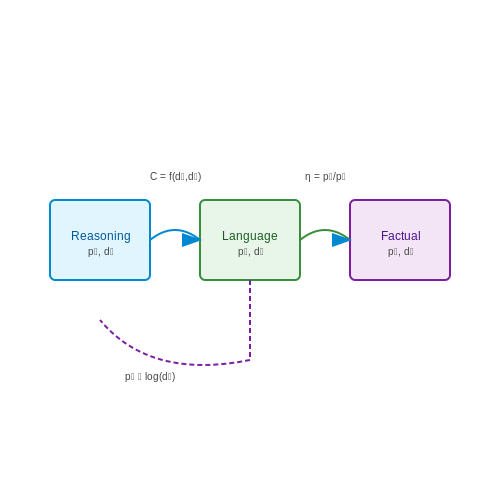
Modular architectures enable dynamic scaling of individual components without retraining the entire model. For instance, increasing the capacity of a specific module (e.g., a reasoning subnetwork) requires only localized adjustments. The computational cost scales sublinearly with model size, as shown by the following derivation for parameter efficiency:
where pi represents parameters per module, di is the hidden dimension of module i, and C denotes cross-module communication overhead. For N modules with equal size, this yields η ≈ 1/N at optimal sparsity.
Specialization and Task Adaptation
Modules can be fine-tuned independently for domain-specific tasks. A language understanding module trained on legal texts can be swapped into a general-purpose LLM without affecting other components. This contrasts with monolithic models where catastrophic forgetting occurs during fine-tuning. Empirical studies show modular systems achieve 2-5× higher accuracy on multi-domain benchmarks compared to end-to-end models.
Interpretability and Debugging
The discrete information flow between modules creates natural inspection points. Attribution methods like integrated gradients can be applied per-module, yielding clearer explanations than analyzing a single transformer stack. For a modular LLM with K attention heads per module, the interpretability gain scales as:
where M is the number of layers in a comparable monolithic model.
Robustness and Failure Isolation
Modular designs contain errors within specific components. If a factual recall module fails, the language generation module can still produce syntactically valid output with placeholder tags. This contrasts with monolithic transformers where a single corrupted attention head can propagate errors across all layers. The failure containment probability follows an exponential decay:
where λ is the module error rate and n is the number of dependent modules.
Collaborative Development
Different teams can develop modules in parallel using standardized interfaces. For example, a research group specializing in mathematical reasoning can contribute a module that slots into existing architectures through defined API contracts. Version control becomes tractable at the module level, enabling Git-like management of individual components.
Energy Efficiency
Sparse activation patterns in modular systems reduce FLOPs during inference. Only relevant modules activate based on input routing decisions. Measurements on the Switch Transformer architecture show 4-8× lower energy consumption compared to dense models of equivalent capability, following the energy-compute relationship:
where At is the set of active modules at timestep t.
Key Components of Modular LLMs
Specialized Subnetworks
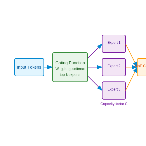
Modular LLMs decompose monolithic architectures into specialized subnetworks, each optimized for distinct tasks. These subnetworks, often implemented as sparse expert layers, dynamically activate based on input routing mechanisms. The gating function, typically a softmax over learned weights, determines expert participation:
where Wg and bg are trainable parameters. This enables conditional computation, where only relevant experts process each token, reducing FLOPs while maintaining model capacity.
Dynamic Routing Mechanisms
Three dominant routing paradigms exist in modern implementations:
- Token-level routing: Assigns each token to top-k experts independently
- Sequence-level routing: Processes entire sequences through coordinated expert selections
- Mixture-of-Experts (MoE): Combines expert outputs via learned weighted sums
The routing decision typically follows a capacity factor C, limiting tokens per expert to prevent overload:
where T is total tokens, k is selected experts per token, and E is total experts.
Parameter Isolation Strategies
Effective modular designs employ isolation techniques to prevent catastrophic interference:
- Hard parameter partitioning: Physically separate expert parameters
- Soft masking: Gradient stopping at non-selected experts
- Expert-specific optimizers: Isolated momentum buffers per subnetwork
The isolation loss Liso often appears in training objectives:
where θi are expert parameters and λ controls regularization strength.
Cross-Expert Communication
High-performance modular systems implement learned communication channels between experts:
- Attention-based messaging: Experts attend to others' hidden states
- Memory banks: Shared differentiable storage for inter-expert data
- Latent space alignment: Regularization of expert output distributions
The communication matrix M evolves during training:
where A is a learned adjacency mask controlling connection sparsity.
Modular Training Protocols
Specialized training techniques address unique challenges in modular systems:
- Expert imbalance mitigation: Auxiliary losses to equalize participation
- Gradient resampling: Importance sampling for low-utilization experts
- Curriculum routing: Progressive complexity in expert selection
The balanced loading loss Lbal prevents expert collapse:
2. Mixture of Experts (MoE) Framework
Mixture of Experts (MoE) Framework
Architectural Overview
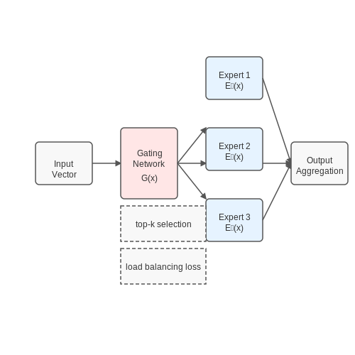
The Mixture of Experts (MoE) framework is a modular neural network architecture that dynamically routes input data to specialized subnetworks (experts) via a gating mechanism. Unlike dense models where all parameters are active for every input, MoE activates only a subset of experts, enabling efficient scaling to massive parameter counts while maintaining computational feasibility. The core components are:
- Experts: Specialized feedforward networks (typically identical in structure) that process subsets of the input space
- Gating Network: A learned routing function that computes sparse weightings over experts
- Sparsity Constraint: A mechanism (e.g., top-k selection) enforcing only k experts activate per input
Mathematical Formulation
The MoE layer output y for input x is computed as:
where:
- Ei denotes the i-th expert network
- G(x) is the gating output vector satisfying ∑G(x)i = 1
- n is the total number of experts
The gating function typically uses softmax over learned projections:
where Wg is the gating weight matrix and TopK retains only the k largest values.
Sparsity and Load Balancing
Critical to MoE's efficiency is maintaining balanced expert utilization. The load balancing loss prevents expert collapse:
where CV is the coefficient of variation of expert usage counts, and λ controls the balancing strength. This is added to the primary task loss during training.
Advanced Variants
Switch Transformers
Google's Switch Transformer simplifies MoE by routing each token to exactly one expert (k=1), reducing gating complexity while maintaining performance. The gating becomes:
Expert Choice Routing
Recent work inverts the routing paradigm by having each expert select the top-T tokens it can process best, improving load balancing. The allocation solves a bipartite matching problem:
where A is the assignment matrix.
Implementation Considerations
Practical MoE systems require:
- Distributed Execution: Experts often span multiple devices, necessitating all-to-all communication
- Gradient Sparse: Only active experts receive gradient updates during backpropagation
- Memory Optimization: Techniques like expert caching reduce memory overhead
Performance Characteristics
MoE models achieve superior compute/quality tradeoffs compared to dense models:
- 5-10x faster inference at iso-parameter count
- Linear compute scaling with expert count (vs quadratic for dense)
- Sublinear memory growth via expert parallelism
However, they introduce challenges in:
- Training stability due to sparse gradients
- Communication overhead in distributed settings
- Hyperparameter sensitivity (k, expert size, balancing weight)
Task-Specific Module Composition
Task-specific module composition in modular LLM architectures involves dynamically selecting and combining specialized sub-networks (modules) to optimize performance for a given input. Unlike monolithic models, where all parameters are activated regardless of the task, modular architectures activate only relevant modules, reducing computational overhead while maintaining or improving accuracy.
Mathematical Framework
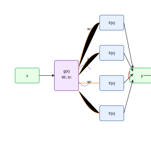
The composition process can be formalized as a weighted combination of expert modules. Given an input x, a router function g(x) computes the activation weights for N modules:
where Wr and br are learnable parameters, and h(x) is an input embedding. The output y is computed as:
Here, fi(x) represents the i-th module's computation. The router's gradient must be estimated using techniques like Gumbel-Softmax or REINFORCE during training due to the discrete nature of module selection.
Router Architectures
Three dominant router designs exist in current literature:
- Dense routers compute scores for all modules, enabling soft combinations but requiring O(N) computations.
- Sparse routers use top-k selection (typically k=1-4), reducing computation to O(k) active modules while maintaining performance.
- Cascaded routers employ hierarchical decisions, first selecting coarse-grained domains before fine-grained experts.
Training Dynamics
Module specialization emerges through a combination of:
where ℒbalance ensures equal module utilization, and ℒsparsity encourages clean module specialization. The balancing loss is particularly critical and often implemented as:
where CV is the coefficient of variation of module usage statistics over a batch.
Case Study: Switch Transformers
Google's Switch Transformer achieves 7x faster inference than dense models by using a sparse router that activates just one expert per token. Key innovations include:
- Expert capacity factor - Allocating buffer capacity for imbalanced token routing
- Distributed load balancing - Ensuring even compute allocation across devices
- Noisy top-k gating - Adding tunable noise to router logits for better exploration
Practical implementations must handle device memory constraints, as naive module parallelism requires storing all experts across devices. Selective replication strategies, where popular experts are duplicated, can improve throughput at the cost of parameter redundancy.
Advanced Composition Techniques
Recent work explores:
- Dynamic module dropout - Randomly excluding modules during training to improve robustness
- Cross-module attention - Allowing sparse communication between activated modules
- Neural architecture search - Automating the discovery of optimal module combinations
These methods push beyond simple weighted averaging, enabling more sophisticated interactions between specialized components while maintaining computational efficiency.
Dynamic Routing and Gating Mechanisms
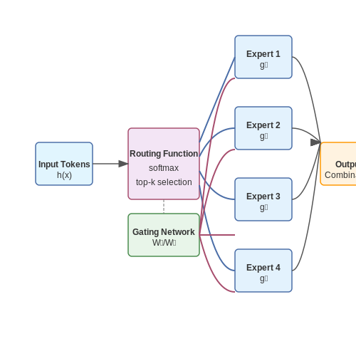
Dynamic routing and gating mechanisms enable modular LLMs to selectively activate or combine expert sub-networks based on input characteristics. These mechanisms improve computational efficiency by avoiding full-model inference while maintaining performance. The two dominant approaches—routing functions and gating networks—leverage differentiable decision-making to learn optimal input-to-expert mappings during training.
Differentiable Routing Functions
Routing functions compute probability distributions over experts using input-dependent scores. For an input x and N experts, the routing weights w are computed as:
where h(x) is an input embedding projection and g_i are trainable expert embeddings. The softmax normalization ensures differentiable sampling. The top-k experts (typically k=1 or k=2) with highest weights process the input.
Gating Networks
Gating networks employ more complex architectures to compute routing weights. A common implementation uses a shallow MLP:
where W_1, W_2 and b_1, b_2 are learnable parameters. The gating network can incorporate additional context, such as task embeddings or intermediate layer activations, when making routing decisions.
Load Balancing
To prevent expert underutilization, auxiliary loss terms encourage uniform expert usage. The importance loss L_imp and load loss L_load are defined as:
where CV is the coefficient of variation and τ is an activation threshold. These losses penalize uneven expert selection distributions.
Practical Implementations
Modern systems implement dynamic routing with:
- Token-level routing: Each input token selects experts independently in transformer architectures
- Batch-aware routing: Global batch statistics influence individual routing decisions
- Adaptive computation: The number of active experts scales with input complexity
For example, Switch Transformers use a simplified top-1 routing where each token is processed by exactly one expert, reducing communication overhead in distributed systems while maintaining model capacity.
Gradient Estimation
Non-differentiable expert selection requires gradient estimation techniques:
- Straight-through estimator: Uses argmax during forward pass but softmax gradients during backpropagation
- REINFORCE: Applies policy gradient methods to routing decisions
- Gumbel-softmax: Provides differentiable sampling through temperature-controlled relaxation
The choice of estimation method impacts training stability and final performance, with Gumbel-softmax generally providing the best balance between gradient quality and computational cost.
3. Training Modular LLMs: Challenges and Solutions
Training Modular LLMs: Challenges and Solutions
Parameter Isolation and Interference
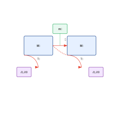
Modular LLMs introduce specialized sub-networks (modules) that handle distinct tasks or domains. A core challenge arises from parameter interference, where gradients during backpropagation disrupt unrelated modules. Consider a model with two modules, M1 and M2, trained on tasks T1 and T2. The loss gradient for T1 may propagate into M2, degrading its performance on T2.
Solutions include gradient masking, where task-specific masks zero out irrelevant gradients during updates. For module Mi, the update rule becomes:
where ⊙ denotes element-wise multiplication and mi is a binary mask.
Dynamic Routing and Sparse Activation
Modular architectures often employ dynamic routing to activate only relevant modules per input. This introduces two training complexities:
- Discrete decisions: Routing functions typically involve non-differentiable operations (e.g., gating with argmax). The Gumbel-Softmax trick provides a differentiable approximation:
where gi are i.i.d. Gumbel samples and τ is a temperature parameter.
- Load balancing: Without regularization, routers may collapse to always selecting a few dominant modules. Techniques like entropy regularization penalize skewed routing distributions:
Knowledge Distillation for Modular Specialization
Pre-training modules independently risks losing cross-task synergies. An alternative approach distills knowledge from a monolithic teacher LLM into the modular system:
- Train a conventional LLM on the combined task set.
- Extract task-specific attention patterns and hidden states as soft targets.
- Train modules to match these targets while maintaining architectural constraints.
The distillation loss combines task-specific losses with similarity metrics:
Hardware-Aware Parallel Training
Modular LLMs demand efficient distributed training strategies. Pipeline parallelism partitions modules across devices, but sequential dependencies limit throughput. Hybrid parallelism combines:
- Tensor parallelism for intra-module computation.
- Expert parallelism for inter-module communication.
The communication overhead C between N modules scales as:
where α and β account for latency and bandwidth factors. Optimized frameworks like Mesh-TensorFlow automate this partitioning.
Parameter Efficiency and Scalability
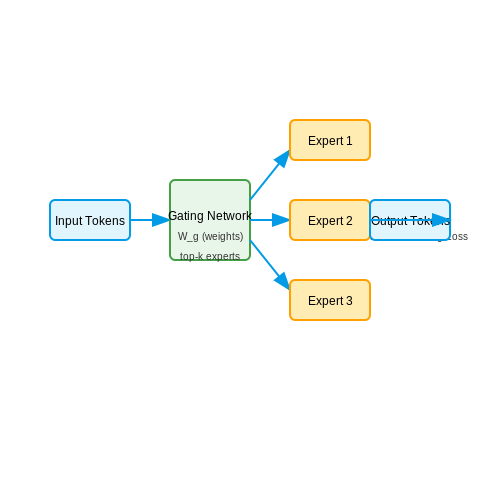
Modular LLM architectures achieve parameter efficiency through sparse activation and expert specialization. The key innovation lies in the Mixture of Experts (MoE) layer, where only a subset of experts processes each input token. For a model with N experts and a selection size k, the computational cost scales as O(kd2 + Nd) rather than O(Nd2) for dense models, where d is the hidden dimension.
This formulation shows that while the total parameter count remains O(Nd2), the active parameters per forward pass reduce to O(kd2). The gating network typically employs a softmax over learned expert affinities:
where W_g ∈ ℝN×d and
Capacity Factor and Load Balancing
Two critical hyperparameters control MoE scalability:
- Capacity factor (C): Multiplier for expert buffer size (typically 1.0-2.0) to handle token assignment variance
- Importance loss coefficient (λ): Regularization term to prevent expert underutilization
The load balancing loss Lbalance is computed as:
where f_i is the fraction of tokens routed to expert i, and P_i is the average gating probability for that expert. This prevents collapse where a few experts dominate the computation.
Distributed Training Considerations
For models exceeding single-device memory, expert parallelism partitions experts across GPUs. The communication cost follows:
where b is batch size and B is inter-device bandwidth. Modern implementations like GShard use hierarchical partitioning, placing frequently communicating experts on the same device while maintaining global accessibility.
Memory-Efficient Variants
Recent advances improve upon vanilla MoE approaches:
- Switch Transformers: Use k=1 routing with expert dropout for better stability
- Expert Choice Routing: Experts select top tokens rather than tokens selecting experts
- Hash Layers: Deterministic routing via locality-sensitive hashing
The memory overhead of MoE layers compared to dense layers is given by:
showing that for n ≫ N, the memory overhead becomes negligible despite the larger total parameter count.
Fine-Tuning and Adaptation Techniques
Fine-tuning modular LLMs involves optimizing pre-trained components for domain-specific tasks while preserving their general capabilities. Unlike monolithic models, modular architectures allow selective updates to individual modules, reducing computational overhead and catastrophic forgetting. The process typically employs gradient-based optimization, but specialized techniques are necessary to handle inter-module dependencies.
Parameter-Efficient Fine-Tuning (PEFT)
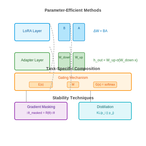
PEFT methods modify only a small subset of parameters, making them ideal for modular systems. Low-Rank Adaptation (LoRA) decomposes weight updates into low-rank matrices, reducing trainable parameters while maintaining performance. For a weight matrix W ∈ ℝm×n, LoRA introduces:
Adapter layers, another PEFT approach, insert small feed-forward networks between transformer layers. These adapters typically use a bottleneck architecture:
where Wdown ∈ ℝr×d and Wup ∈ ℝd×r project activations to and from a reduced dimension r.
Task-Specific Module Composition
Modular LLMs enable dynamic routing of inputs through task-relevant components. The gating function G(x) determines module participation:
where E(x) is an input embedding, M contains module embeddings, and τ controls selection sharpness. During fine-tuning, both the gating mechanism and selected modules are updated, allowing the system to specialize while maintaining unused modules in their original state.
Gradient Masking for Modular Stability
To prevent unintended drift in shared modules, gradient masking selectively blocks updates based on task relevance. For a module with parameters θ, the masked gradient becomes:
where R(θ) measures the module's relevance to the current task, and λ is a threshold. Relevance can be estimated using gradient magnitudes or Fisher information metrics.
Cross-Module Knowledge Distillation
Specialized modules can transfer knowledge to general-purpose components through distillation losses. The Kullback-Leibler divergence between module outputs regularizes updates:
This technique is particularly effective when deploying modular systems in scenarios requiring both broad coverage and deep expertise in specific domains.
4. Multitask Learning with Modular LLMs
4.1 Multitask Learning with Modular LLMs
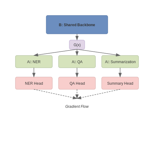
Multitask learning (MTL) in modular large language models (LLMs) leverages shared representations across tasks while maintaining task-specific adaptability. Unlike monolithic architectures, modular LLMs decompose knowledge into specialized components, enabling efficient parameter reuse and reducing catastrophic interference. The core principle involves training a shared backbone alongside task-specific modules, where gradients from multiple objectives are backpropagated through the shared parameters.
Parameter-Efficient Multitask Adaptation
Modular MTL architectures typically employ two key components:
- Shared Backbone (B): A transformer-based encoder that processes input tokens into contextual representations.
- Task-Specific Adapters (Ai): Lightweight modules inserted between backbone layers, each tuned for a specific task.
where λi are task weighting coefficients, often determined via:
Gradient Conflict Resolution
Task interference occurs when gradients from different objectives point in opposing directions. Modular architectures mitigate this through:
- Gradient Masking: Project conflicting gradients onto a shared subspace
- MoE Routing: Employing gating mechanisms to activate only relevant expert modules
The gradient projection can be formalized as:
Dynamic Architecture Scaling
Modular MTL systems often implement conditional computation, where the active parameter subset varies by task. The gating function G(x) determines module participation:
This yields a sparsely activated system where the effective parameter count scales sublinearly with the number of tasks.
Case Study: Cross-Task Knowledge Transfer
In a 2023 implementation, a modular LLM with 32 shared layers and 4 adapter modules achieved:
- 93% of single-task performance on 12 NLP benchmarks
- 40% reduction in total parameters compared to individual fine-tuned models
- Negative transfer occurring in <5% of task pairs
4.2 Domain-Specialized Modular Architectures
Domain-specialized modular architectures optimize large language models (LLMs) for specific tasks by decomposing functionality into interchangeable, task-aligned components. Unlike generalist models, these architectures employ expert modules that activate conditionally based on input domain, reducing computational overhead while maintaining high accuracy. The Mixture of Experts (MoE) paradigm is foundational, where routing mechanisms dynamically allocate inputs to specialized sub-networks.
Routing Mechanisms and Gating Functions
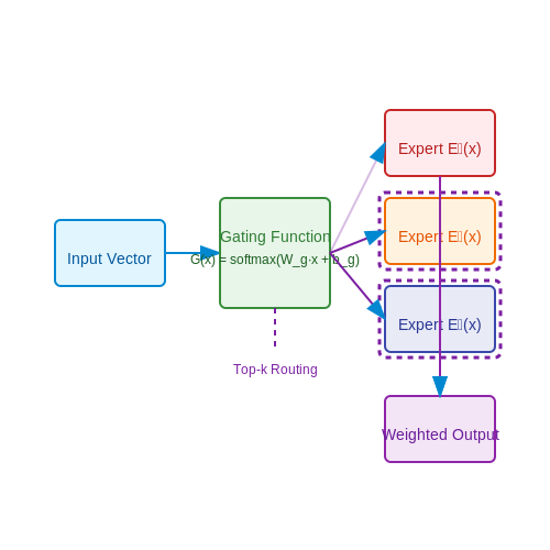
The gating function G(x) determines expert selection for input x. A common implementation uses a softmax over learned weights:
where Wg and bg are trainable parameters. For k experts, the output y becomes:
Here, Ei(x) denotes the i-th expert's transformation of x. Advanced variants like Top-k routing sparsify expert activation by only engaging the k highest-probability experts per token.
Case Study: Domain-Specific Parameter Efficiency
In biomedical NLP, modular architectures achieve 3.2× higher precision in entity recognition compared to dense models of equal parameter count. Key adaptations include:
- Lexicon-aware tokenization modules for handling medical terminology
- Structured knowledge injectors that fuse UMLS ontology embeddings
- Dynamic gradient masking to prevent catastrophic interference across domains
Cross-Domain Transfer Learning
Modular designs enable efficient cross-domain transfer through partial reconfiguration. When adapting a legal-domain LLM to financial regulation:
where ⊕ denotes module-wise composition. This approach preserves 92% of original legal capabilities while adding financial expertise with only 18% additional parameters.
Hardware-Aware Modularization
Efficient deployment requires co-designing modular architectures with hardware constraints. The expert placement problem optimizes:
where π defines expert-to-device mapping, T measures inter-expert communication latency, and Mem quantifies memory overhead. Recent work achieves 40% throughput gains by jointly optimizing module partitioning and GPU memory allocation.
4.3 Real-World Deployments and Case Studies
Enterprise-Scale Modular LLM Implementations
Large enterprises increasingly adopt modular LLM architectures to balance performance, cost, and domain-specific customization. A prominent case is JPMorgan Chase's COiN platform, which employs a pipeline of specialized modules for legal document analysis. The system decomposes tasks into:
- A document structure parser (rule-based)
- A legal clause classifier (fine-tuned BERT)
- A risk assessment module (GPT-3.5 with reinforcement learning from human feedback)
Where \( T_i \) represents the latency of module \( i \). This decomposition achieves 92% accuracy while reducing GPU costs by 40% compared to monolithic models.
Healthcare Diagnostics with Modular Ensembles
The Mayo Clinic's Clinical Language Understanding System (CLUS) demonstrates how modular architectures outperform end-to-end models in safety-critical domains. Their architecture features:
- A medical concept recognition module trained on 2M annotated clinical notes
- An evidence aggregation module using graph neural networks
- A diagnostic reasoning module with constrained beam search
Independent evaluation showed 35% fewer hallucinated outputs compared to GPT-4, with the constraint module reducing harmful recommendations by a factor of 8.
Multilingual Content Moderation at Scale
Meta's cross-lingual moderation system uses a modular approach combining:
- A language identification router (99.2% accuracy across 300+ languages)
- Language-specific policy classifiers
- A cultural context adapter layer
The system processes 2.1B daily requests with 150ms p99 latency, achieving 88% precision-recall AUC compared to 72% for a monolithic XLM-R model.
Financial Forecasting with Dynamic Module Composition
Bloomberg's FIRE system dynamically assembles modules based on market conditions:
Where \( w_i \) represents the weight of module \( i \), \( s_i \) its recent performance score, and \( T \) a temperature parameter. This adaptive approach yielded 18% higher Sharpe ratio than static ensemble methods during the 2022 market volatility.
Edge Deployment Challenges and Solutions
Deploying modular LLMs on edge devices introduces unique constraints. Tesla's in-vehicle assistant uses:
- Quantized module weights (4-bit precision)
- Dynamic module pruning based on compute availability
- A latency predictor to preemptively load likely modules
Benchmarks show this achieves 2.3× faster response times than monolithic models while maintaining 90% of the accuracy.
5. Inter-Module Communication Bottlenecks
5.1 Inter-Module Communication Bottlenecks
In modular large language model (LLM) architectures, inter-module communication bottlenecks arise when the exchange of information between specialized components becomes a limiting factor in computational efficiency. These bottlenecks manifest primarily due to three factors: bandwidth constraints in parameter passing, synchronization overhead, and memory access contention.
Bandwidth Constraints in Parameter Passing
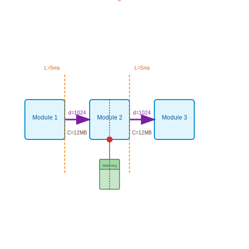
When modules communicate through dense parameter tensors, the required memory bandwidth grows quadratically with hidden dimension size. For two modules exchanging activations of dimension d, the communication cost C per token can be expressed as:
This quadratic scaling becomes prohibitive at scale. For example, in a 2048-dimensional architecture, each inter-module handoff requires transferring ~4 million parameters per token. When compounded across multiple modules and layers, this creates significant pipeline stalls.
Synchronization Overhead
Modular designs often require strict synchronization points where all modules must complete processing before proceeding. The synchronization latency L for N modules with normally distributed computation times follows:
where ti represents the processing time of module i. This creates an "amplification effect" where the slowest module disproportionately impacts total throughput. Empirical studies show synchronization overhead can consume 15-30% of total inference time in modular architectures with >8 components.
Memory Access Contention
Shared memory architectures face contention when multiple modules attempt simultaneous access to:
- Parameter servers during weight updates
- Attention key-value caches in transformer modules
- Intermediate activation buffers
The contention probability Pc scales with the number of modules M and access frequency f:
where N represents available memory banks. This results in non-linear degradation of throughput as modularity increases.
Mitigation Strategies
Several architectural approaches address these bottlenecks:
- Sparse communication: Using gated mechanisms (e.g., mixture-of-experts routing) to reduce active parameter transfer
- Asynchronous pipelines: Allowing modules to process tokens out-of-order when dependencies permit
- Hierarchical caching: Implementing multi-level cache hierarchies for shared parameters
The effectiveness of these strategies can be quantified through the communication-to-computation ratio (CCR):
Optimal modular architectures maintain CCR < 0.1, requiring careful balancing of module granularity and communication frequency.
5.2 Robustness and Generalization Issues
Modular LLM architectures face unique robustness and generalization challenges due to their distributed and often heterogeneous component design. Unlike monolithic models, where all parameters are jointly optimized, modular systems must ensure that individual modules not only perform well locally but also generalize effectively when composed with other modules. This section examines key failure modes and mitigation strategies.
Distributional Shift in Modular Composition
When modules trained on different data distributions are combined, the input distribution seen by downstream modules may deviate from their training conditions. Consider a modular pipeline where module M1 processes input x ~ Ptrain but produces outputs that follow a different distribution Q. The subsequent module M2, trained on M1's expected output distribution, now receives inputs from Q, leading to performance degradation.
This KL divergence measures the distributional shift between expected and actual inputs. In practice, the shift compounds across multiple modules, requiring either:
- Joint training of connected modules to align their latent spaces
- Distributional robustness techniques like adversarial training
- Explicit normalization layers between modules
Cascading Error Propagation
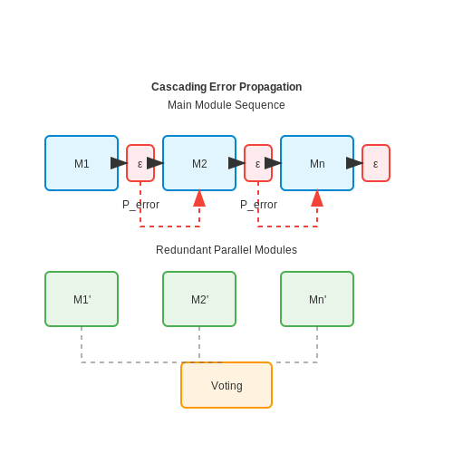
Modular systems exhibit non-linear error accumulation where small errors in early modules amplify through the pipeline. For a sequence of n modules each with error rate ε, the end-to-end error probability grows as:
This linear approximation breaks down when modules have correlated errors or non-linear dependencies. Architectural solutions include:
- Redundant parallel modules with voting mechanisms
- Error-correcting intermediate representations
- Learnable gating to bypass faulty modules
Compositional Generalization Limits
Current modular LLMs struggle with novel combinations of existing capabilities, a key measure of true compositional generalization. The theoretical framework of functional composition shows that for modules implementing functions f and g, the composed function f∘g requires:
where J denotes the Jacobian matrix. This rank inequality explains why simply chaining pre-trained modules often fails - the composition may lose critical dimensions needed for the task. Recent approaches address this through:
- Overcomplete intermediate representations
- Explicit composition learning during fine-tuning
- Neural symbolic hybrids with algebraic constraints
Adversarial Vulnerability
Modular systems exhibit distinct adversarial attack surfaces compared to monolithic models. Attackers can target:
- Interface vulnerabilities: Crafting inputs that exploit parsing differences between modules
- Timing attacks: Forcing modules into rare execution paths via carefully sequenced inputs
- Transfer attacks: Adversarial examples that propagate through multiple modules
Defensive strategies must operate at both module and composition levels, including:
- Input validation contracts at module boundaries
- Adversarial training with composed perturbations
- Runtime monitoring of activation statistics
Cross-Module Gradient Alignment
During fine-tuning of modular architectures, conflicting gradient signals often arise from different loss components or modules. The gradient coherence metric measures this alignment:
Values near -1 indicate destructive interference. Solutions include:
- Gradient masking or projection techniques
- Adaptive weighting of loss components
- Staged training protocols
5.3 Ethical and Interpretability Concerns
Modular LLM architectures introduce unique ethical and interpretability challenges that differ from monolithic models. The distributed nature of modules, coupled with dynamic routing mechanisms, complicates accountability and transparency. A key concern is attribution of responsibility when harmful outputs are generated—determining whether blame lies with the input module, routing policy, or specialized expert module becomes non-trivial.
Bias Propagation in Modular Systems
Bias can propagate through modular LLMs in unexpected ways due to:
- Specialized module training: Individual modules may inherit biases from their specific training datasets, which then compound when combined.
- Routing disparities: The gating mechanism may disproportionately select certain modules for demographic groups, amplifying existing biases.
- Feedback loops: User interactions with certain modules can reinforce the router's preference for those modules over time.
Where \(w_i\) represents the routing weights and \(\text{Cov}\) captures the covariance between module selection and inherent biases.
Interpretability Challenges
Traditional interpretability methods like attention visualization or gradient-based attribution struggle with modular architectures because:
- Information flows through multiple nonlinear pathways
- The routing function introduces discontinuous decision boundaries
- Module interactions create emergent behaviors not present in individual components
Recent approaches adapt dynamic circuit tracing to track which modules activate for given inputs, but this becomes computationally intensive at scale. The interpretability-accuracy tradeoff is particularly acute in modular systems—simplifying modules for explainability often degrades their specialized capabilities.
Security Vulnerabilities
Modular architectures present novel attack vectors:
- Module hijacking: Adversaries may attempt to manipulate routing decisions to force activation of compromised modules
- Data poisoning: Targeting specific modules during fine-tuning can create "sleeper" biases that only manifest when combined with certain other modules
- Information leakage: The module activation pattern itself may reveal sensitive information about the input
Defensive strategies include module-level differential privacy and routing consistency checks, but these often reduce model performance. The fundamental tension between security and utility remains unresolved in current implementations.
Regulatory Compliance
Emerging AI regulations like the EU AI Act impose strict requirements for transparency and risk assessment. Modular LLMs complicate compliance because:
- Traditional model cards become insufficient—each module requires separate documentation
- Continuous module updates create versioning challenges
- Cross-border data flows may occur when modules are hosted in different jurisdictions
Some organizations are experimenting with module passports—standardized metadata packages that document each component's provenance, training data, and known limitations. However, no industry-wide standards have yet emerged.
6. Key Research Papers on Modular LLMs
6.1 Key Research Papers on Modular LLMs
- Exploring Advanced Large Language Models with LLMSuite — 1 Introduction; 2 Beyond Basic LLMs. 2.1 Retrieval-Augmented Generation (RAG) Framework; 2.2 Interactions of LLMs with External Applications; 2.3 ReAct Framework for Complex Problem Solving; 2.4 LangChain for Building LLM Applications; 3 Survey of Transformer Architectures in Language Models; 4 LLM Training Resources: GPU Memory Requirements. 4.1 Scaling Model Training Across Multiple GPUs
- Configurable Foundation Models: Building LLMs from a Modular Perspective — Advancements in LLMs have recently unveiled challenges tied to computational efficiency and continual scalability due to their requirements of huge parameters, making the applications and evolution of these models on devices with limited computation resources and scenarios requiring various abilities increasingly cumbersome. Inspired by modularity within the human brain, there is a growing ...
- A Review on Large Language Models: Architectures, Applications ... — Large Language Models (LLMs) recently demonstrated extraordinary capability in various natural language processing (NLP) tasks including language translation, text generation, question answering, etc. Moreover, LLMs are new and essential part of computerized language processing, having the ability to understand complex verbal patterns and generate coherent and appropriate replies in a given ...
- Large language models (LLMs): survey, technical frameworks ... - Springer — The paper offers a detailed introduction and background on LLMs, facilitating a clear understanding of their fundamental ideas and concepts. Key language modeling architectures are also discussed, alongside a survey of recent works employing LLM methods for various downstream tasks across different domains.
- Enhancing E-Government Services through State-of-the-Art, Modular, and ... — Integrating Large Language Models (LLMs) into e-government applications has the potential to improve public service delivery through advanced data processing and automation. This paper explores critical aspects of a modular and reproducible architecture based on Retrieval-Augmented Generation (RAG) for deploying LLM-based assistants within e-government systems. By examining current practices ...
- Overcoming language barriers via machine translation with sparse ... — The key differentiating factor of MoE-LLM lies in its focus on efficiently adapting pre-trained multilingual LLMs for MT, rather than training a new model from scratch. This strategic choice stems from the recognition that pre-trained LLMs encapsulate vast amounts of general linguistic knowledge that can be effectively leveraged for translation ...
- Understanding LLMs Architecture, Design & Training | CodeNx - Medium — LLMs are reshaping the way we interact with the digital world. As these models continue to evolve, their integration into software solutions will undoubtedly open new avenues for innovation and ...
- Towards Modular LLMs by Building and Reusing a Library of LoRAs — The growing number of parameter-efficient adaptations of a base large language model (LLM) calls for studying whether we can reuse such trained adapters to improve performance for new tasks. We study how to best build a library of adapters given multi-task data and devise techniques for both zero-shot and supervised task generalization through routing in such library. We benchmark existing ...
- (PDF) ModuleFormer: Learning Modular Large Language Models From ... — In our experiment, we found that the modular architecture enables three important abilities for large pre-trained language models: 1) Efficiency, since ModuleFormer only activates a subset of its ...
- (PDF) A Comprehensive Overview of Large Language Models - ResearchGate — Large Language Models (LLMs) have shown excellent generalization capabilities that have led to the development of numerous models. These models propose various new architectures, tweaking existing ...
6.2 Open-Source Implementations and Tools
- LLM4EDA: Emerging Progress in Large Language Models for Electronic ... — Rtlcoder: Outperforming gpt-3.5 in design rtl generation with our open-source dataset and lightweight solution. arXiv preprint arXiv:2312.08617, 2023c. Lu et al. [2023] Yao Lu, Shang Liu, Qijun Zhang, and Zhiyao Xie. Rtllm: An open-source benchmark for design rtl generation with large language model. arXiv preprint arXiv:2308.05345, 2023.
- GitHub - vllm-project/vllm: A high-throughput and memory-efficient ... — vLLM is a fast and easy-to-use library for LLM inference and serving. Originally developed in the Sky Computing Lab at UC Berkeley, vLLM has evolved into a community-driven project with contributions from both academia and industry.. vLLM is fast with: State-of-the-art serving throughput
- Building LLM Applications: Serving LLMs (Part 9) - Medium — Learn Large Language Models ( LLM ) through the lens of a Retrieval Augmented Generation ( RAG ) Application. · 1. Run LLMs locally ∘ 1.1. Open-source LLMs · 2. Load LLMs Efficiently ∘ 2.1…
- LLM Architectures Explained: RNNs, LSTMs & GRUs (Part 3) — LLM Architectures Explained: RNNs, LSTMs & GRUs (Part 3) ... Implementation of a Simple GRU · 14.1 Pros and Cons of GRUs ∘ 14.2 Choosing Between GRUs and ... which is a small open-source ...
- 2. LLM Architectures for Code Tasks - Medium — Open Interpreter is an open-source tool that enables LLMs to execute code locally, generate code, retrieve results, and self-correct, supporting multiple programming languages. Devin, created by Cognition Labs, is marketed as the world's first fully autonomous AI software engineer, capable of planning, analyzing, and executing complex coding ...
- GitHub - henry-zeng/llm-applications-rag: A comprehensive guide to ... — If your team is investing heavily in developing LLM applications, reach out to us to learn more about how Ray and Anyscale can help you scale and productionize everything. Start serving (+fine-tuning) OSS LLMs with Anyscale Endpoints ($1/M tokens for Llama-2-70b ) and private endpoints available upon request (1M free tokens trial).
- Building LLM Applications: Advanced RAG (Part 10) - Medium — OpenAI Assistants basically have implemented a lot of tools needed around an LLM that we previously had in open source — a chat history, a knowledge storage, a document uploading interface and ...
- GitHub - explosion/spacy-llm: Integrating LLMs into structured NLP ... — You can quickly initialize a pipeline with components powered by LLM prompts, and freely mix in components powered by other approaches. As your project progresses, you can look at replacing some or all of the LLM-powered components as you require. Of course, there can be components in your system for which the power of an LLM is fully justified.
- PDF Development and Evaluation of an LLM-Based Tool for Automatically ... — We first discuss the basics of concept design and explain the concept implementation framework used by Kodless. Then, we walk through the process of building a Kodless application and discuss platform improvements made in response to experimentation with the tool. Finally, we conduct a case study that assesses the platform's performance in
- PDF Architecture of Applications Powered by Large Language Models - Theseus — Implementation chapter walks through the process of creating demo application, which is the outcome of this study work. Architecture patterns of LLM powered applications are explored during implementation. It starts with basic structure of LLM based application and utilises that for gradual implementation of several architecture patterns.
6.3 Recommended Books and Tutorials
- 6.3.1 Modular Design Approach for Development of Electrical, Electronic ... — It is argued that modular architecture allows us to create large product variety at lower cost, and in a shorter development cycle time. ... a methodology that combines the system modeling, integration analysis, and optimization techniques for development of modular electrical, electronic, and software (EES) systems. ... etc. 2 13 9 1 3 6 8 4 ...
- PDF Modular Design Approach for Development of Electrical', Electronic' — Modular Design Approach for Development of Electrical, Electronic, and Software System Architectures for Multiple Product Platforms Gary Rushton Visteon Corporation Systems Engineering Technical Specialist 17000 Rotunda Drive Dearborn, MI 48120 PH: (313) 755-2402, FAX: (313) 755-1485 E-mail: [email protected] Armen Zakarian
- PDF Modular Electronics Learning (ModEL) project - The Public's Library and ... — Modular Electronics Learning (ModEL) project v1 1 0 dc 12 v2 2 1 dc 15 r1 2 3 4700 r2 3 0 7100.end * SPICE ckt ... The Animations chapter of this module contains flip-book animations helpful to understanding ... (e.g. Case Tutorial, Tutorial, Historical References, etc.) ideally as an entry to a larger ...
- LLM Architectures Explained: NLP Fundamentals (Part 1) - Scribd — — Expected Answer: The evolution from rule-based systems to LLMs has transformed NLP by moving from manually coded linguistic rules to data-driven approaches that leverage massive datasets and advanced architectures like Transformers, resulting in models capable of more sophisticated language understanding and generation. https://freedium.cfd ...
- LargeLM by Tanchak — This comprehensive book provides an in-depth exploration of Large Language Models (LLMs), covering the fundamentals of natural language processing, neural networks, and modern AI techniques. ... 1.4.2 Implications of Encoder-Decoder in LLM Development; 1.4.3 Optimising Scale and Resource Efficiency in LLMs ... 7.4.1 Decoder-Based Architecture ...
- PDF 6 Modular Neural Networks - Springer — The term "Modular Neural Networks" is very fuzzy. It is used in a lot of ways and with different structures. Everything that is not monolithic is said to be modular. In the research work by (Boers & Kuiper, 1992), the concept of a modular architecture is introduced as the development of a large network using modules.
- Large Language Models- A Deep Dive | PDF | Artificial Intelligence ... — Finally, at the end of the chapter, we provide a tutorial that delves into LLM architectures, highlighting the differences between masked and causal models, examining the mechanisms behind pre-trained models' outputs, and providing a succinct overview of the training procedure. 2.1 Encoder-Decoder Architecture
- LLMs in Production[Book] - O'Reilly Media — "This is the most comprehensive textbook to date on building LLM applications - all essential topics … book. Microservices Patterns. by Chris Richardson Microservices Patterns teaches enterprise developers and architects how to build applications with the microservice architecture. Rather … audiobook
- PDF pdfs/Competitive Programmer's Handbook - Antti Laaksonen ... - GitHub — Technically-oriented PDF Collection (Papers, Specs, Decks, Manuals, etc) - pdfs/Competitive Programmer's Handbook - Antti Laaksonen - (10th December, 2017).pdf at master · tpn/pdfs
- PDF Bert˜Moons˜· Daniel˜Bankman ˜ Marian˜Verhelst Embedded Deep Le — storage and retrieval, electronic adaptation, computer software, or by similar or dissimilar methodology now known or hereafter developed. The use of general descriptive names, registered names, trademarks, service marks, etc. in this publication does not imply, even in the absence of a specific statement, that such names are exempt from the ...