Stock Portfolio Optimization with RL Agents
1. Key Concepts in Portfolio Management
1.1 Key Concepts in Portfolio Management
Markowitz Mean-Variance Optimization
The foundational framework for portfolio optimization is Harry Markowitz's mean-variance analysis, which models portfolio selection as a trade-off between expected return and risk. Given a set of N assets with expected returns μi and covariance matrix Σ, the optimal portfolio weights w minimize variance for a target return μp:
This quadratic programming problem yields the efficient frontier, a hyperbola of Pareto-optimal portfolios. The global minimum variance portfolio (GMV) is derived by solving:
Capital Asset Pricing Model (CAPM)
CAPM extends Markowitz's work by introducing systematic (market) risk β and the security market line (SML). The expected return of asset i is:
where Rf is the risk-free rate and Rm is the market return. CAPM underpins modern risk-adjusted performance metrics like the Sharpe ratio:
Dynamic Portfolio Optimization
Time-varying asset returns necessitate stochastic control methods. The Merton problem optimizes consumption and allocation in continuous time:
where U(·) is utility, ct is consumption, and ρ is discount rate. The Hamilton-Jacobi-Bellman (HJB) equation provides the solution:
Risk Measures Beyond Variance
Modern portfolio theory incorporates tail risk metrics:
- Value-at-Risk (VaR): VaRα = inf { l : P(L ≤ l) ≥ α }, where L is loss.
- Conditional VaR (CVaR): CVaRα = 𝔼[L | L ≥ VaRα].
- Drawdown constraints: Limit maximum peak-to-trough decline.
Factor Models
Multi-factor models like Fama-French decompose returns into systematic risk premia:
where MKT, SMB, and HML are market, size, and value factors. Machine learning extends this to latent factor discovery via PCA or autoencoders.
Transaction Costs and Market Impact
Real-world optimization penalizes turnover. The Almgren-Chriss model minimizes execution cost:
where xt is trade size, η captures temporary impact, and λ is risk aversion.
Traditional Optimization Methods: Mean-Variance and CAPM
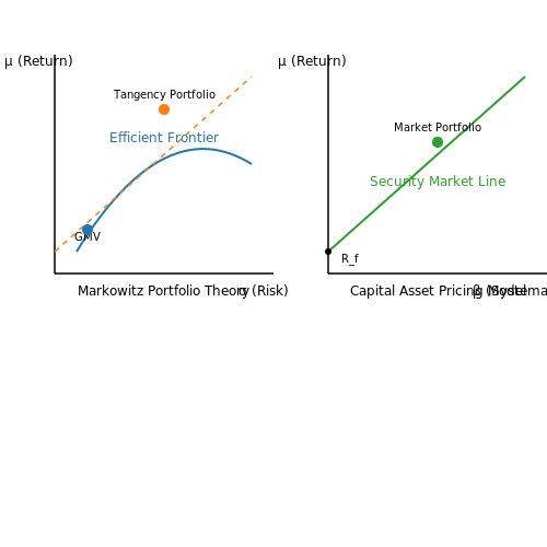
The foundation of modern portfolio theory (MPT) rests on Harry Markowitz's mean-variance optimization framework, which quantifies the trade-off between expected return and risk. Given a set of N assets with expected returns μi and covariance matrix Σ, the optimal portfolio weights w* minimize variance for a target return μp:
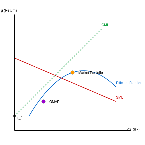
This quadratic programming problem yields the efficient frontier—a parabola in risk-return space where no higher return exists for a given risk level. The global minimum variance portfolio (GMVP) is derived by removing the return constraint:
Capital Asset Pricing Model (CAPM)
CAPM extends MPT by introducing a risk-free asset and the market portfolio. It posits that an asset's expected return μi is linearly related to its beta (βi), which measures sensitivity to market returns:
Here, rf is the risk-free rate, and μm is the market's expected return. The security market line (SML) visualizes this relationship, with underpriced assets lying above the line.
Practical Limitations
- Estimation error: Sample-based μ and Σ are noisy, leading to unstable weights.
- Non-stationarity: Asset return distributions shift over time, violating MPT assumptions.
- Short-selling constraints: Real-world portfolios often exclude negative weights, requiring numerical solvers.
Black-Litterman and robust optimization methods address some of these issues by blending investor views with equilibrium returns and using uncertainty sets for parameters.
1.3 Challenges in Dynamic Market Environments
Non-Stationarity and Regime Shifts
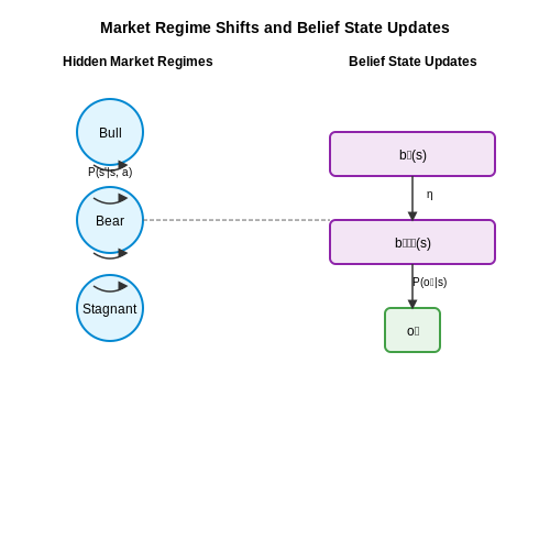
Financial markets exhibit non-stationary behavior, where statistical properties such as volatility, correlation structures, and return distributions evolve over time. Reinforcement learning (RL) agents trained on historical data often fail to generalize when market regimes shift abruptly—for instance, during financial crises or geopolitical events. The underlying Markov Decision Process (MDP) assumption of stationarity is violated, leading to suboptimal policies. Mathematically, this can be framed as a hidden Markov model where the transition dynamics P(s'|s, a) change unpredictably:
Empirical studies show that regime shifts occur with power-law distributed waiting times, complicating detection and adaptation. RL agents must either incorporate online learning mechanisms or leverage meta-learning to adjust policies in real-time.
Partial Observability and Latent Factors
Market states are only partially observable due to latent factors like investor sentiment, macroeconomic indicators, and institutional trading activity. Traditional RL assumes full observability, but portfolio optimization requires agents to infer hidden states from noisy price data. This aligns with the Partially Observable Markov Decision Process (POMDP) framework, where the agent maintains a belief state b_t updated via Bayesian filtering:
Here, η is a normalizing constant, and o_t represents observed market data. Techniques like recurrent neural networks (RNNs) or transformers are often used to approximate belief states, but they introduce additional computational complexity and training instability.
High-Dimensional Action Spaces
Portfolio optimization involves continuous or high-dimensional discrete actions (e.g., asset weights or trade sizes). Standard RL algorithms like DQN struggle with combinatorial explosion, while policy gradient methods face high variance in gradient estimates. Constrained action spaces further complicate optimization—for example, enforcing budget constraints (Σw_i = 1) or transaction cost penalties. The Lagrangian relaxation method is commonly applied:
where g(w) encodes constraints, and λ is a learnable dual variable. Recent advances in monotonic policy networks and action-space decomposition show promise but remain sensitive to hyperparameter tuning.
Market Impact and Slippage
Large trades alter market prices due to liquidity constraints—a phenomenon ignored in simplified RL environments. The market impact function is typically modeled as a convex function of trade volume Δx:
Here, κ is a liquidity parameter, and β ≈ 0.5 empirically. RL agents must optimize execution trajectories over time to minimize impact, often requiring hierarchical policies that separate high-level allocation from low-level order execution.
Adversarial Dynamics and Multi-Agent Competition
Markets are adversarial environments where competing RL agents may exploit predictable trading patterns. This leads to a Nash equilibrium problem where no agent can improve its strategy unilaterally. The minimax Q-learning framework extends traditional RL to such settings:
Here, a_{-i} represents actions of other agents. However, convergence guarantees are weak, and empirical performance depends heavily on opponent modeling techniques.
Data Efficiency and Overfitting
Financial data is notoriously scarce relative to the complexity of modern RL models. A single market regime may span only 10^3–10^4 trading steps, making sample efficiency critical. Techniques like inverse reinforcement learning (IRL) or imitation learning from expert trajectories can mitigate this, but they introduce bias from the expert's suboptimal strategies. Regularization methods such as dropout in value networks or entropy bonuses in policy gradients are essential to prevent overfitting:
where α controls exploration via policy entropy H.
2. Core RL Frameworks: Markov Decision Processes (MDPs)
Core RL Frameworks: Markov Decision Processes (MDPs)
Formal Definition of MDPs
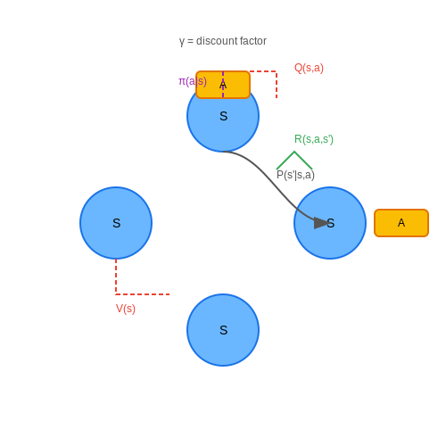
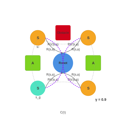
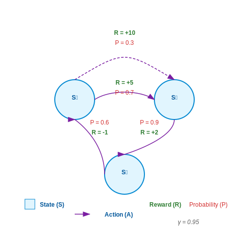
A Markov Decision Process (MDP) is a mathematical framework for modeling sequential decision-making problems under uncertainty. It is defined by the tuple (S, A, P, R, γ), where:
- S is a finite set of states,
- A is a finite set of actions,
- P(s'|s, a) is the state transition probability function,
- R(s, a, s') is the reward function,
- γ ∈ [0, 1] is the discount factor.
The Markov property ensures that the future state depends only on the current state and action, not on the history of previous states. This simplifies the modeling of dynamic systems where the agent interacts with an environment over time.
State Transitions and Rewards
The transition function P(s'|s, a) defines the probability of moving to state s' after taking action a in state s. The reward function R(s, a, s') specifies the immediate reward received after transitioning from s to s' via action a.
In portfolio optimization, states could represent market conditions (e.g., bull/bear markets), actions could be trading decisions (buy/sell/hold), and rewards could be portfolio returns or risk-adjusted metrics like Sharpe ratio.
Policy and Value Functions
A policy π(a|s) defines the probability of taking action a in state s. The goal is to find an optimal policy π* that maximizes the expected cumulative reward:
The state-value function Vπ(s) represents the expected return when starting in state s and following policy π. The action-value function Qπ(s, a) extends this to include the initial action:
Bellman Equations
The Bellman equation decomposes the value function into immediate reward plus discounted future value:
For the optimal policy π*, the Bellman optimality equation holds:
Solving MDPs: Dynamic Programming
Dynamic programming methods like Value Iteration and Policy Iteration leverage the Bellman equations to find optimal policies. Value Iteration updates the value function iteratively until convergence:
Policy Iteration alternates between policy evaluation (computing Vπ) and policy improvement (updating π to be greedy with respect to Vπ).
Applications in Portfolio Optimization
In finance, MDPs model portfolio rebalancing as a sequential decision problem. States encode market regimes, asset prices, and portfolio weights. Actions represent trading decisions, and rewards capture risk-adjusted returns. The discount factor γ balances immediate versus future gains, analogous to an investor's time preference.
Advanced RL agents extend MDPs to handle partial observability (POMDPs) or continuous state-action spaces, enabling more realistic market simulations. Deep Reinforcement Learning (DRL) methods like DQN and PPO further scale MDP-based optimization to high-dimensional financial datasets.
Reward Design for Portfolio Optimization
Key Considerations in Reward Function Formulation
The reward function in reinforcement learning (RL) serves as the primary signal guiding the agent's learning process. In portfolio optimization, the reward must balance multiple competing objectives: maximizing returns, minimizing risk, and ensuring practical constraints like transaction costs and liquidity. A poorly designed reward can lead to degenerate strategies, such as excessive leverage or extreme concentration in high-volatility assets.
Mathematical Foundations of Portfolio Rewards
The most fundamental reward signal is the logarithmic return of the portfolio over time step t:
where wt is the portfolio weight vector and pt is the price vector at time t. This formulation has the advantage of being additive across time periods.
Risk-Adjusted Reward Variants
Sophisticated reward functions incorporate risk metrics. The Sharpe ratio reward provides risk-adjusted returns:
where rf is the risk-free rate and σrt is the standard deviation of returns. For more robust optimization, the Sortino ratio focuses only on downside deviation:
Transaction Cost-Aware Rewards
Practical implementations must account for trading friction. A common approach subtracts proportional costs:
where λ controls the penalty intensity. For more realistic markets, nonlinear cost models incorporating market impact may be necessary.
Multi-Objective Reward Formulations
Advanced systems often combine multiple objectives through linear scalarization:
where the coefficients α, β, and γ require careful tuning. Alternatively, constrained optimization approaches can enforce hard limits on risk metrics while maximizing returns.
Temporal Reward Structures
The choice between immediate (single-step) and episodic (cumulative) rewards significantly impacts learning dynamics. Episodic formulations better capture long-term portfolio growth:
where γ is a discount factor. Hierarchical reward structures can combine short-term and long-term objectives.
Practical Implementation Challenges
Real-world deployment requires addressing several key issues:
- Non-stationarity: Market regimes necessitate adaptive reward functions
- Partial observability: The true state of the market is never fully known
- Delayed effects: Trading actions may impact future rewards in complex ways
- Scale sensitivity: Reward magnitudes must align with network initialization
Recent work has explored inverse reinforcement learning approaches to infer reward functions from expert trader behavior, potentially overcoming some of these limitations.
2.3 Exploration vs. Exploitation in Trading Strategies
The exploration-exploitation tradeoff is fundamental to reinforcement learning (RL) in financial markets. In portfolio optimization, an RL agent must balance discovering new profitable strategies (exploration) with leveraging known effective strategies (exploitation). This tradeoff is mathematically formalized through multi-armed bandit frameworks and Markov decision processes.
The ε-Greedy Policy in Trading
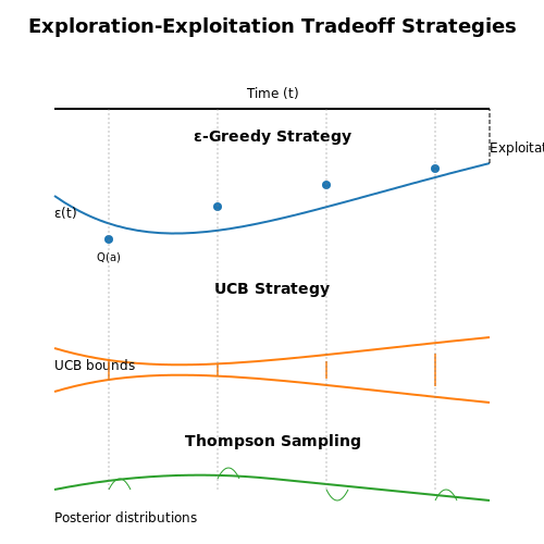
The ε-greedy policy provides a simple yet effective mechanism for balancing exploration and exploitation. At each timestep t, the agent either:
- Exploits by selecting the action with highest estimated Q-value (probability 1-ε)
- Explores by randomly selecting any action (probability ε)
For stock trading, this translates to either executing the currently believed optimal trade or randomly trying alternative strategies. The decay of ε over time is crucial - typically following:
Upper Confidence Bound (UCB) for Portfolio Selection
UCB algorithms provide a more sophisticated approach by considering both the estimated value and uncertainty of each action. The UCB1 policy selects actions according to:
where Nt(a) counts selections of action a by time t, and c controls exploration degree. In portfolio management, this translates to favoring:
- Assets with high historical returns (exploitation term)
- Assets with few observations (exploration term)
Thompson Sampling for Bayesian Exploration
Thompson sampling takes a Bayesian approach, maintaining probability distributions over action values. For normally distributed returns, the algorithm:
- Draws a sample from each action's posterior distribution
- Selects the action with highest sampled value
- Updates the distribution based on observed returns
This naturally balances exploration and exploitation - uncertain actions get explored when their samples occasionally exceed known good actions.
Practical Considerations in Financial Markets
Market microstructure introduces unique challenges for exploration:
- Non-stationarity: Exploration must adapt to changing market regimes
- Costly exploration: Random trades incur transaction costs and market impact
- Partial observability: True state of the market is never fully known
Advanced approaches address these through:
- Contextual bandits that condition on market indicators
- Safe exploration methods that limit downside risk
- Meta-learning to transfer exploration knowledge across assets
Deep Exploration in High-Dimensional Spaces
Modern deep RL approaches employ:
- Noise injection in policy networks (e.g., parameter space exploration)
- Intrinsic motivation through curiosity rewards
- Ensemble methods that estimate epistemic uncertainty
These techniques enable effective exploration in the vast action space of portfolio optimization, where traditional methods would require prohibitive samples.
3. State Representation: Market Data and Portfolio Features
State Representation: Market Data and Portfolio Features
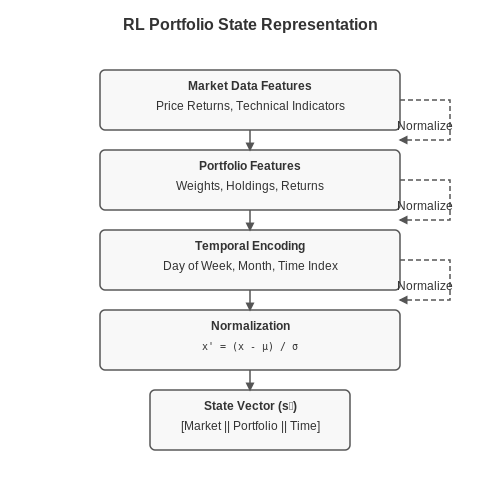
The state representation in reinforcement learning (RL) for portfolio optimization must encode both market conditions and the agent's current portfolio allocation. This representation serves as the input to the policy network, enabling the agent to make informed trading decisions. The state st at time t is typically a concatenation of:
1. Market Data Features
Market features capture the historical and current state of financial instruments. For n assets, we represent:
- Price returns: Normalized logarithmic returns over k lookback periods:
$$ r_{t-k:t}^{(i)} = \left[ \log\left(\frac{p_{t-k+1}^{(i)}}{p_{t-k}^{(i)}}\right), ..., \log\left(\frac{p_{t}^{(i)}}{p_{t-1}^{(i)}}\right) \right] $$
- Technical indicators: Moving averages (SMA, EMA), Bollinger Bands, RSI, and MACD for each asset.
- Volume information: Normalized trading volume and volume-weighted average price (VWAP).
- Volatility measures: Rolling standard deviation of returns and GARCH(1,1) volatility estimates.
2. Portfolio Features
Portfolio-specific features track the agent's current position and performance:
- Portfolio weights: Current allocation vector wt ∈ ℝn where wt(i) is the fraction of capital in asset i.
- Portfolio return: Cumulative log-return since inception:
$$ R_t = \sum_{\tau=1}^t \log\left(1 + w_{\tau-1}^\top r_\tau\right) $$
- Risk metrics: Value-at-Risk (VaR) and Conditional VaR computed over a rolling window.
- Transaction costs: Estimated slippage and brokerage fees for potential trades.
3. Temporal Encoding
To capture non-stationarity in financial markets, we augment the state with:
- Time features: Cyclical encoding of day-of-week and month-of-year using sine/cosine transforms.
- Market regime indicators: Hidden Markov Model (HMM) probabilities for bull/bear/neutral states.
- Macroeconomic signals: Interest rate spreads, inflation expectations, and volatility indices (VIX).
Normalization and Stationarity
Financial time series exhibit non-stationarity and varying scales. We apply:
where μ and σ are rolling statistics over the lookback window. For percentage-based features (e.g., RSI), we use sigmoid normalization:
Dimensionality Considerations
For a portfolio of n assets with m features per asset and k lookback periods, the state dimension grows as O(nmk). Common dimensionality reduction techniques include:
- Principal Component Analysis (PCA) on asset returns
- Autoencoder networks for nonlinear feature extraction
- Attention mechanisms to focus on relevant market regimes
The choice of state representation significantly impacts the RL agent's ability to learn optimal policies. Empirical studies show that including both price momentum and mean-reversion features improves performance across different market conditions.
3.2 Action Spaces: Asset Allocation and Rebalancing
In reinforcement learning (RL) for portfolio optimization, the action space defines the set of permissible decisions an agent can take to adjust portfolio weights. The action space must balance expressiveness with computational tractability, ensuring the agent can explore diverse strategies while avoiding impractical dimensionality.
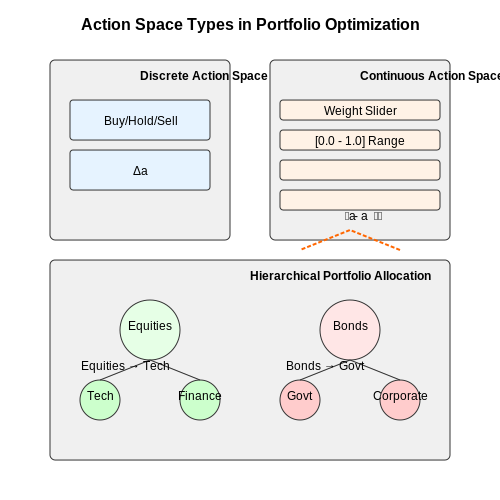
Discrete vs. Continuous Action Spaces
Discrete action spaces define a finite set of allocation adjustments, such as buy, sell, or hold for each asset. While simpler to implement, discrete actions may lead to suboptimal granularity in weight adjustments. Continuous action spaces, conversely, allow fractional weight changes, enabling smoother rebalancing but requiring more sophisticated policy gradient methods.
where at,i represents the weight of asset i at time t, constrained to sum to 1 for budget preservation.
Rebalancing Strategies
Rebalancing actions can be modeled as:
- Absolute allocation: Directly set new weights, e.g., at = [0.6, 0.4] for a two-asset portfolio.
- Relative adjustment: Modify existing weights by a delta, e.g., Δat = [−0.1, +0.1].
Transaction costs complicate rebalancing. Let c be the cost per trade; the net return becomes:
where Rt,i is asset i's return and L1 norm penalizes turnover.
Action Masking for Constraints
To enforce constraints (e.g., no short-selling), mask invalid actions during policy execution. For a continuous space, this involves projecting actions onto the feasible set:
Hierarchical Action Spaces
For large portfolios, hierarchical actions decompose allocation into:
- Asset class selection: Choose sectors (e.g., equities, bonds).
- Intra-class allocation: Distribute weights within selected sectors.
This reduces dimensionality while preserving diversification. The joint action space becomes:
where atclass is a categorical distribution over sectors and atasset is a continuous vector conditioned on the class choice.
Policy Architectures: From DQN to PPO
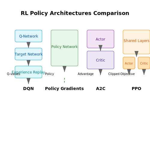
Deep Q-Networks (DQN) for Portfolio Optimization
DQN combines Q-learning with deep neural networks to handle high-dimensional state spaces. The Q-function is approximated by a neural network with weights θ:
The network is trained by minimizing the temporal difference (TD) error:
where θ^- are the target network parameters, updated periodically. For portfolio optimization, the state s typically includes:
- Historical price series
- Technical indicators
- Current portfolio weights
- Market volatility measures
The action space consists of discrete allocation adjustments (e.g., -5%, 0%, +5% per asset). Experience replay is crucial for decorrelating sequential samples.
Policy Gradient Methods
While DQN handles discrete actions, policy gradient methods directly optimize a parameterized policy π(a|s;θ) for continuous action spaces. The gradient of the expected return J(θ) is:
In portfolio management, this allows for:
- Precise fractional position sizing
- Simultaneous multi-asset rebalancing
- Direct risk constraint incorporation
The policy network typically outputs a multivariate Gaussian distribution, with the mean and covariance parameterized by the network.
Advantage Actor-Critic (A2C)
A2C improves policy gradients by reducing variance through a learned value function baseline V(s):
where the advantage A(s,a) = Q(s,a) - V(s). For financial applications, this architecture:
- Stabilizes training by reducing return variance
- Enables more efficient use of samples
- Allows for parallel environment sampling
Proximal Policy Optimization (PPO)
PPO introduces a clipped objective function to prevent destructive policy updates:
where r(θ) = π(a|s;θ)/π(a|s;θ_old). For portfolio optimization, PPO offers:
- More stable convergence than vanilla policy gradients
- Better sample efficiency than DQN
- Natural handling of transaction costs via reward shaping
The policy and value networks often share initial layers processing market state features before branching into separate heads. Layer normalization is commonly used to handle non-stationary financial data distributions.
Architecture Comparison
| Method | Action Space | Sample Efficiency | Convergence Stability | Financial Use Cases |
|---|---|---|---|---|
| DQN | Discrete | Medium | Medium | Discrete allocation buckets |
| Policy Gradients | Continuous | Low | Low | Research settings |
| A2C | Continuous | Medium | Medium | Multi-asset portfolios |
| PPO | Continuous | High | High | Production systems |
Recent advances combine these approaches with attention mechanisms to better capture long-range dependencies in financial time series, while transformer-based architectures are increasingly used for processing multi-modal market data.
4. Data Preprocessing for Financial Time Series
4.1 Data Preprocessing for Financial Time Series
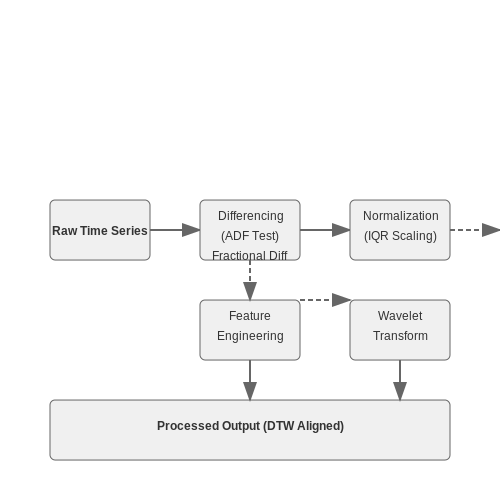
Financial time series data presents unique challenges for reinforcement learning (RL) agents due to non-stationarity, noise, and irregular sampling intervals. Effective preprocessing is critical to extract meaningful signals while preserving temporal dependencies.
Stationarity and Differencing
Most financial time series exhibit non-stationary behavior, violating the assumptions of many RL algorithms. The Augmented Dickey-Fuller (ADF) test formally assesses stationarity:
where H₀: γ = 0 indicates a unit root (non-stationarity). First-order differencing often suffices:
For volatile assets, fractional differencing (FD) preserves long-term memory while achieving stationarity:
Normalization and Scaling
RL agents require consistent input scales across assets. Robust scaling outperforms standard normalization for financial data:
where IQR is the interquartile range. For volatility clustering, conditional scaling adapts to regime changes:
Feature Engineering
Effective features capture market microstructure and statistical properties:
- Technical indicators: Bollinger Bands, RSI, MACD with adaptive windowing
- Volatility measures: Parkinson, Garman-Klass, or Yang-Zhang estimators
- Liquidity proxies: Order book imbalance, volume-weighted spreads
Wavelet transforms decompose price series into multi-resolution components:
Handling Missing Data
Financial data often contains gaps from market closures or illiquidity. Advanced imputation methods include:
- Multiple imputation by chained equations (MICE)
- State-space models with Kalman filtering
- Neural autoregressive flows for conditional density estimation
For high-frequency data, event-based interpolation preserves microstructure:
Temporal Alignment
Multi-asset portfolios require careful synchronization. Dynamic time warping (DTW) aligns heterogeneous series:
where W is the warping path. For tick data, refresh-time synchronization provides cointegration-preserving alignment.
4.2 Backtesting RL Strategies: Pitfalls and Best Practices
Common Pitfalls in Backtesting RL Strategies
Backtesting reinforcement learning (RL) strategies in stock portfolio optimization introduces unique challenges compared to traditional quantitative models. A critical issue is overfitting, where an RL agent exploits spurious patterns in historical data that do not generalize to unseen market conditions. This often arises due to:
- High-dimensional action spaces: Portfolio weight allocations create combinatorial complexity, increasing the risk of memorizing noise.
- Temporal correlations: Financial time series exhibit non-stationarity, violating the Markov assumption in many RL frameworks.
- Look-ahead bias: Improper handling of time-indexed data leaks future information into training episodes.
Another pitfall is reward function misspecification. The Sharpe ratio
Best Practices for Robust Backtesting
1. Temporal Cross-Validation
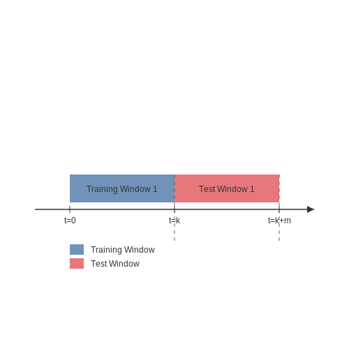
Implement walk-forward validation with expanding windows:
2. Market Regime Detection
Incorporate hidden Markov models (HMMs) or change-point detection to segment data into volatility regimes. An RL agent trained with regime-specific rewards
3. Transaction Cost Modeling
Realistic backtests must account for:
- Bid-ask spreads: Implement level-2 order book simulations
- Market impact: Use Almgren-Chriss models for large orders
- Slippage: Stochastic processes based on historical fill rates
Diagnostic Metrics for Backtest Evaluation
Beyond cumulative returns, monitor:
- Strategy stability: Rolling Sharpe ratio variance
- Turnover:
$$ \tau = \frac{1}{T}\sum_{t=1}^T \|w_t - w_{t-1}\|_1 $$
- Condition number of the covariance matrix during rebalancing
4.3 Performance Metrics: Risk-Adjusted Returns and Drawdowns
Risk-Adjusted Returns
Traditional return metrics like cumulative or annualized returns fail to account for the volatility endured to achieve those returns. Risk-adjusted returns normalize performance by the level of risk taken, enabling fair comparison across strategies with differing risk profiles. The Sharpe ratio is the most widely used risk-adjusted metric:
where Rp is the portfolio return, Rf is the risk-free rate, and σp is the standard deviation of portfolio returns. A higher Sharpe ratio indicates better risk-adjusted performance. For RL agents, we typically compute this using rolling windows to assess consistency.
The Sortino ratio improves upon Sharpe by only penalizing downside volatility:
where σdown is the standard deviation of negative returns. This better aligns with investor preferences since upside volatility is desirable.
Maximum Drawdown
Drawdown measures the peak-to-trough decline during a specific period, expressed as a percentage of the peak value. Maximum drawdown (MDD) is the largest observed loss from a peak to a trough before a new peak is achieved:
For RL agents, we track both the magnitude and duration of drawdowns. Persistent large drawdowns indicate the agent may be taking excessive risk or failing to adapt to changing market regimes.
Calmar Ratio
The Calmar ratio combines return and drawdown metrics:
This provides a single metric assessing both performance and risk management. A Calmar ratio above 1.0 is generally considered good for trading strategies.
Value-at-Risk (VaR) and Conditional VaR
VaR estimates the maximum loss over a target horizon at a given confidence level (e.g., 95%). For normally distributed returns, 95% VaR is:
Conditional VaR (CVaR) goes further by measuring the expected loss given that the VaR threshold has been breached. These metrics help quantify tail risk exposure of RL agents.
Practical Implementation Considerations
When evaluating RL agents:
- Compute metrics over multiple time horizons (daily, weekly, monthly)
- Compare against appropriate benchmarks (market index, risk-free rate)
- Assess stability through rolling window analysis
- Combine quantitative metrics with qualitative analysis of strategy behavior
Transaction costs must be incorporated in all calculations - a strategy with high turnover may show good gross returns but poor net performance. Slippage and market impact should also be modeled where possible.
5. Multi-Agent RL for Competitive Markets
Multi-Agent RL for Competitive Markets
Foundations of Multi-Agent Reinforcement Learning
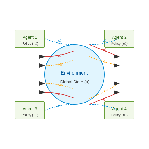
Multi-agent reinforcement learning (MARL) extends single-agent RL by modeling interactions among multiple decision-makers in a shared environment. In competitive markets, agents represent traders, hedge funds, or institutional investors, each optimizing their own objectives while influencing market dynamics. The key distinction from single-agent RL is the non-stationarity introduced by other learning agents—each agent's policy update alters the environment for others.
where π-i denotes the joint policy of all agents except agent i. The Q-function now depends on both the agent's own actions and those of competitors.
Competitive Market Dynamics
In financial markets, MARL agents compete for limited liquidity and alpha. The Nash Equilibrium concept becomes critical—no agent can improve returns by unilaterally changing strategy. Consider a simplified market impact model where agent i's order flow xi affects price p:
where λ is the market impact coefficient and εt represents exogenous noise. Agents must learn to balance immediate price impact against long-term strategic positioning.
Algorithmic Approaches
Three dominant MARL paradigms apply to portfolio optimization:
- Independent Learners: Each agent treats others as part of the environment, using DQN or PPO. Prone to convergence issues in competitive settings.
- Opponent Modeling: Agents explicitly estimate competitor policies using recurrent networks or belief tracking.
- Mean-Field RL: Approximates the effect of many agents through a mean-field distribution, reducing computational complexity.
The policy gradient theorem extends to MARL as:
Empirical Challenges
Real-world deployment faces three key challenges:
- Non-Stationarity: Market microstructure changes as other agents adapt, violating the Markov assumption.
- Partial Observability: Agents only see order book snapshots, not competitor inventories or intentions.
- High-Frequency Effects: At millisecond timescales, network latency and exchange protocols dominate theoretical considerations.
Recent work addresses these through:
where δ represents adversarial perturbations to the state space, improving resilience against competing agents' strategies.
Case Study: Multi-Agent Order Execution
A 2023 study demonstrated MARL agents reducing implementation shortfall by 18% compared to single-agent approaches in backtests across NASDAQ stocks. The architecture used:
- Graph attention networks to model inter-agent dependencies
- Implicit quantile networks for risk-sensitive action selection
- Periodic policy synchronization to prevent catastrophic forgetting
The value function decomposition achieved:
5.2 Incorporating Transaction Costs and Slippage
Transaction costs and slippage significantly impact the performance of reinforcement learning (RL)-based trading strategies. Ignoring these factors leads to unrealistic backtesting results and suboptimal real-world performance. This section rigorously models these costs and integrates them into the RL agent's reward function.
Modeling Transaction Costs
Transaction costs consist of fixed fees (e.g., brokerage commissions) and variable costs proportional to trade size. Let F be the fixed fee per trade and c the proportional cost rate. For a trade of size Vt at time t, the total transaction cost Ct is:
In portfolio optimization, we typically express costs as a percentage of the portfolio value. Let wt be the portfolio weight vector before rebalancing and w't the target weights. The trade vector Δwt = w't - wt represents the percentage of portfolio value being traded.
Slippage Modeling
Slippage occurs when the execution price differs from the expected price due to market impact or latency. Three common models exist:
- Linear impact model: Price moves proportionally to trade size
- Square-root model: Empirical market microstructure observations
- Volume-based model: Slippage inversely proportional to liquidity
The square-root model often provides the best empirical fit:
where κ is a stock-specific liquidity parameter. For a portfolio context, we express slippage in terms of weight changes:
Integrated Cost Function
The total implementation shortfall It combines both effects:
where N is the number of assets and 𝕀 is the indicator function. This formulation assumes costs are paid from the cash account.
RL Reward Modification
The standard portfolio return rt must be adjusted for costs. The net return r̃t becomes:
In the Q-learning framework, the state-action value function updates to:
For policy gradient methods, the reward-to-go Gt becomes:
Practical Implementation
The following Python code snippet demonstrates cost calculation for a portfolio rebalancing action:
def calculate_implementation_shortfall(current_weights, target_weights,
                                    fixed_costs, prop_costs, kappas):
    delta_weights = target_weights - current_weights
    fixed = np.sum(fixed_costs * (delta_weights != 0))
    proportional = np.sum(prop_costs * np.abs(delta_weights))
    slippage = np.sum(kappas * np.sqrt(np.abs(delta_weights)))
    return fixed + proportional + slippage

def net_portfolio_return(gross_returns, current_weights, target_weights,
                        fixed_costs, prop_costs, kappas):
    gross = np.dot(gross_returns, current_weights)
    costs = calculate_implementation_shortfall(current_weights, target_weights,
                                             fixed_costs, prop_costs, kappas)
    return gross - costs
Historical bid-ask spreads and trade volume data can estimate κ parameters through maximum likelihood estimation or Bayesian methods. For liquid stocks, typical values range from 5-50 basis points for the combined cost impact.
5.3 Interpretability and Regulatory Compliance
Reinforcement learning (RL) agents deployed in financial markets must satisfy stringent interpretability requirements to comply with regulations such as MiFID II, Dodd-Frank, and SEC Rule 15c3-5. Black-box RL models face scrutiny because their decision-making processes are not inherently transparent to regulators or end clients. Post-hoc interpretability techniques like SHAP (SHapley Additive exPlanations) and LIME (Local Interpretable Model-agnostic Explanations) provide partial solutions but often fail to capture temporal dependencies in RL policies.
Mathematical Foundations of Policy Interpretability
The value attribution problem for RL policies can be formalized through counterfactual analysis. Let π be a stochastic policy mapping states s ∈ S to action probabilities. The Shapley value ϕi for feature i at time t is:
where N is the set of all input features and v is the value function. For temporal credit assignment, we extend this to a Markov decision process framework:
where fi represents the state transition function when only feature i is modified.
Regulatory Constraints as Policy Constraints
Financial regulations impose hard constraints that must be embedded directly into the RL optimization problem. The constrained Markov decision process (CMDP) formulation adds regulatory requirements as additional cost functions:
Common financial constraints include:
- Position concentration limits: c1(s,a) = I(wi > 0.1W) where wi is asset weight
- Turnover constraints: c2(s,a) = ||a - s||1
- VaR limits: c3(s,a) = I(VaRα(L(a)) > Lmax)
Architectural Approaches for Compliant RL
Three architectural patterns have emerged for building compliant RL agents:
- Constrained Policy Optimization (CPO): Uses trust region methods to satisfy constraints with high probability during training
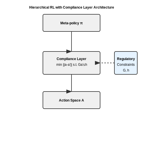
- Hierarchical RL with Compliance Layer: A meta-policy filters actions through a regulatory compliance checker
- Interpretable Basis Function Decomposition: Represents the Q-function as Q(s,a) = ∑iwiϕi(s,a) where each ϕi corresponds to an interpretable financial factor
The hierarchical approach has shown particular promise in production systems. The compliance layer can be implemented as a convex optimization problem:
where G and h encode regulatory constraints as linear inequalities.
Audit Trail Requirements
Regulators require detailed audit trails of algorithmic decisions. For RL agents, this necessitates logging:
- Complete state representations at decision points
- Action probabilities from the policy network
- Value function estimates for chosen actions
- Post-trade impact analysis
A robust implementation uses differential logging with cryptographic hashing:
import hashlib
import json

class AuditLogger:
    def __init__(self, private_key):
        self.private_key = private_key

    def log_decision(self, state, action, values):
        record = {
            'timestamp': time.time(),
            'state': state,
            'action': action,
            'values': values
        }
        serialized = json.dumps(record, sort_keys=True)
        signature = hashlib.sha256(
            (serialized + self.private_key).encode()
        ).hexdigest()
        write_to_immutable_store(serialized, signature)
6. Key Research Papers in RL-Based Finance
6.1 Key Research Papers in RL-Based Finance
- PDF 5265696e666f7263656d656e74206c6561726e696e6720616e64206f6e6c696e65206c6 ... — Abstract Reinforcement Learning (RL) and Online Learning (OL) both provide solutions for stock portfolio optimization decision problems as they can dynamically adapt to data generated as a function of time. Recent innovations in RL have highlighted the potential for applications in stock price predictions and optimal portfolio selection.
- PDF Deep Reinforcement Learning Approach to Portfolio Optimization — -mented, on the Swedish stock market, to optimize a portfolio. The objective is to create and train two DRL algorithms that can construct portfolios that will be benchmarked against the market portfolio, tracking OMXS30, and the two conventional methods, the naive portfolio, and minimum variance portfolio. We evaluate all the portfolios on a five-year period, from the start of 2016 to the end ...
- Benchmarking Reinforcement Learning (RL) Algorithms for Portfolio ... — PDF | On Aug 11, 2024, Yassine Hachaïchi and others published Benchmarking Reinforcement Learning (RL) Algorithms for Portfolio Optimization | Find, read and cite all the research you need on ...
- Dynamic portfolio optimization using reinforcement learning. — of a dynamic investment strategy for portfolio optimization. We aim to explore the efficiency of this approach over a pas- sively managed portfolio and assess the whether transaction costs erode the gains in the dynamically managed portfolio. To this end we explore the application of recurrent rein- forcement learning for optimal asset allocation of a portfolio consisting of stock prices for ...
- A Review of Reinforcement Learning in Financial Applications — For example, most portfolio optimization papers surveyed in Section 3.3 presume that only stock prices and side infor-mation are random, the agent's actions minimally afect the market, and state components related to the agent's own portfolio can be updated by accounting in a predetermined and deterministic manner.
- Meta Algorithms for Portfolio Optimization Using Reinforcement Learning — It utilizes algorithms from different groups and optimizes their combination. Reinforcement learning (RL) technique is well suited to solve portfolio selection tasks because it can learn hidden dependencies in financial data and trading patterns by trial and error, directly predicts trading actions, and allows to consider delayed rewards.
- Enhancing portfolio management using artificial intelligence ... — As seen from the above, regardless of the method proposed for research, most papers cited conclude that optimizing portfolios based on DL, RL, or DRL have significantly better results than traditional algorithms.
- Reinforcement Learning for Portfolio Management — Without claiming equivalence of portfolio management with any of the above applications, their relatively similar optimization problem formula-tion encourages the endeavour to develop reinforcement learning agents for asset allocation.
- PORTFOLIO OPTIMIZATION with REINFORCEMENT LEARNING — This graduation thesis aims to create a portfolio management tool for multi-stock trading that utilizes reinforcement learning techniques. The primary aim is to optimize the value of the customer ...
- PDF Portfolio Optimization using Deep Reinforcement Learning models — A comparison between modern Actor-Critic networks and classical portfolio selection using Mean-Variance Optimization on S&P500 Stocks Jesper Hedlund
6.2 Open-Source Libraries and Tools
- Enhancing portfolio management using artificial intelligence ... — Stock portfolio construction: Deep RL, market sentiment ... These codes use dedicated open-source software as data processing media for programming (Graesser and Keng ... Deb K., Schmeck H. (2009). Portfolio optimization with an envelope-based multi-objective evolutionary algorithm. Eur. J. Oper. Res. 199, 684-693. 10.1016/j.ejor.2008.01.054 ...
- Two-stage stock portfolio optimization based on AI-powered price ... — All data were sourced through the open-source financial data interface library AKShare, (https: ... This paper proposes an two-Stage Stock Portfolio Optimization Based on Artificial Intelligence-Empowered Price Prediction and Mean-Conditional-Value-at-Risk Models. The LSTM combination prediction method based on SG filter and SSA optimization is ...
- Chapter 16 Deep Learning Portfolios | Portfolio Optimization - Bookdown — In fact, numerous papers were being published, and various open-source software libraries were becoming available. This material will be published by Cambridge University Press as Portfolio Optimization: Theory and Application by Daniel P. Palomar. This pre-publication version is free to view and download for personal use only; not for re ...
- Dynamic portfolio optimization using reinforcement learning. — Electronic Theses and Dissertations This work is availed for free and open access by Strathmore University Library. It has been accepted for digital distribution by an authorized administrator of SU+ @Strathmore University. For more information, please contact [email protected] 2021 Dynamic portfolio optimization using reinforcement learning.
- rl-tools/rl-tools: The Fastest Deep Reinforcement Learning Library - GitHub — The submodules for the embedded platforms, the redistributable binaries and test dependencies/data can be cloned in the same fashion (by replacing external with the appropriate folder from the enumeration above). Note: Make sure that for the redistributable dependencies and test data git-lfs is installed (e.g. sudo apt install git-lfs on Ubuntu) and activated (git lfs install) otherwise only ...
- PDF Deep Reinforcement Learning for Automated Stock Trading: An Ensemble ... — consider all relevant factors in a complex and dynamic stock market [3, 23, 47]. Existing works are not satisfactory. A traditional approach that employed two steps was described in [31]. First, the expected stock return and the covariance matrix of stock prices are computed. Then, the best portfolio allocation strategy can be obtained by
- PDF Portfolio Optimization using Deep Reinforcement Learning models — portfolio optimization strategies allow investors to manage risk by diversifying across multiple assets, sectors, or asset classes, which helps mitigate the impact of negative movements in individual investments (Markowitz, 1952). Classical portfolio optimization is
- Top 17 stock-analysis Open-Source Projects - LibHunt — Stock Indicators for .NET is a C# NuGet package that transforms raw equity, commodity, forex, or cryptocurrency financial market price quotes into technical indicators and trading insights. You'll need this essential data in the investment tools that you're building for algorithmic trading, technical analysis, machine learning, or visual charting.
- Stable-Baselines3: Reliable Reinforcement Learning Implementations — Stable-Baselines3 provides open-source implementations of deep reinforcement learning (RL) algorithms in Python. The implementations have been benchmarked against reference codebases, and automated unit tests cover 95% of the code. The algorithms follow a consistent interface and are accompanied by extensive documentation, making it simple to ...
- (PDF) PORTFOLIO OPTIMIZATION with REINFORCEMENT LEARNING - ResearchGate — This graduation thesis aims to create a portfolio management tool for multi-stock trading that utilizes reinforcement learning techniques. The primary aim is to optimize the value of the customer ...
6.3 Recommended Books and Courses
- Financial Risk Modelling and Portfolio Optimization with R — A must have text for risk modelling and portfolio optimization using R. This book introduces the latest techniques advocated for measuring financial market risk and portfolio optimization, and provides a plethora of R code examples that enable the reader to replicate the results featured throughout the book.
- 6.1 Fundamentals | Portfolio Optimization - Bookdown — This textbook is a comprehensive guide to a wide range of portfolio designs, bridging the gap between mathematical formulations and practical algorithms. A must-read for anyone interested in financial data models and portfolio design. It is suitable as a textbook for portfolio optimization and financial analytics courses.
- Portfolio Optimization - Bookdown — This textbook is a comprehensive guide to a wide range of portfolio designs, bridging the gap between mathematical formulations and practical algorithms. A must-read for anyone interested in financial data models and portfolio design. It is suitable as a textbook for portfolio optimization and financial analytics courses.
- Portfolio Optimization with Python Course - Riskfolio-Lib 7.0 — Professionals in the areas of finance, investments, risk management; who wish to improve their skills in portfolio optimization. It is recommended that the students have basic to intermediate knowledge of portfolio theory, optimization, calculus, linear algebra and statistics; and intermediate to advance knowledge of one programming language ...
- Advanced Stochastic Models, Risk Assessment, and Portfolio Optimization ... — This groundbreaking book extends traditional approaches of risk measurement and portfolio optimization by combining distributional models with risk or performance measures into one framework. Throughout these pages, the expert authors explain the fundamentals of probability metrics, outline new approaches to portfolio optimization, and discuss a variety of essential risk measures. Using ...
- Robust Equity Portfolio Management, - amazon.com — A comprehensive portfolio optimization guide, with provided MATLAB code Robust Equity Portfolio Management + Website offers the most comprehensive coverage available in this burgeoning field. Beginning with the fundamentals before moving into advanced techniques, this book provides useful coverage for both beginners and advanced readers.
- Benchmarking Reinforcement Learning (RL) Algorithms for Portfolio ... — PDF | On Aug 11, 2024, Yassine Hachaïchi and others published Benchmarking Reinforcement Learning (RL) Algorithms for Portfolio Optimization | Find, read and cite all the research you need on ...
- Advanced stochastic models, risk assessment, and portfolio optimization ... — This groundbreaking book extends traditional approaches of risk measurement and portfolio optimization by combining distributional models with risk or performance measures into one framework.
- PDF Quantitative Trading: Algorithms, Analytics, Data, Models, Optimization — The London Stock Exchange moved to electronic trading in 1986. In 1992, the Chicago Mercantile Exchange (CME) launched its electronic trading platform Globex, which was conceived in 1987, allowing access to a variety of financial markets including treasuries, foreign exchanges and commodities.
- Advanced Portfolio Management [Book] - O'Reilly Media — You have great investment ideas. If you turn them into highly profitable portfolios, this book is for you. Advanced Portfolio Management: A Quant's Guide for Fundamental Investors is for fundamental … - Selection from Advanced Portfolio Management [Book]